Spin-Hall edge spin polarization in a ballistic 2D electron system

Introduction. Spintronics addresses interplay of spin and orbital degrees of freedom in various transport, optical, etc. phenomena with the ultimate goal of achieving spin manipulation in nanostructures. Special place in spintronics belongs to the spin-Hall effect predicted a long time ago DP, which recently entered the era of experimental observation exp1; exp2; exp3. Spin-Hall effect is characterized by a boundary (edge) spin polarization resulting when electric current is flowing through the system. It is customary classified into “extrinsic” (impurity-driven) H; Z; ERH; DS and “intrinsic” (band-structure induced) MNZ; Sinova types. Initially theories of spin-Hall effect addressed such auxiliary quantity as spin current (for the review see Refs. reviews) in infinite systems, but later the emphasis shifted towards direct calculation of spin polarization in confined geometries. For diffusive systems the search is to complement the coupled spin-density diffusion equations MSH; BNM with suitable boundary conditions Chu; AB; GBD; Blei; Tser; RGD.

While it is now understood that in 2D systems spin-Hall effect generally occurs with more complicated spin-orbit couplings, any amount of disorder destroys spin-Hall effect in infinite systems with linear coupling reviews. It is, therefore, important to establish whether pure ballistic systems (without disorder) can exhibit non-zero spin-Hall polarization. Driven by this motivation, studies of intrinsic spin-Hall effect in ballistic finite-size systems had been initiated, mostly by means of numerical methods NWS; nik. It is significant to realize that the edge spin polarization in ballistic systems appears not as a result of electric field-driven acceleration of electron momenta (and associated with it precession of spins). As well known, electric field is absent inside an ideal ballistic conductor connected to reflectionless leads Datta. Spin-Hall spin accumulation in ballistic systems is due to the edge precession only. When the populations of left-moving and right moving states are different, the boundary scattering results in oscillatory (Friedel) edge polarization which is perpendicular to both the electric current and the normal direction to the boundary. Such polarization was considered numerically in Refs. usaj for a 2D electron gas (2DEG). The case of a 3D hole semiconductor has also been analyzed recently SG. A possibility of distinguishing edge effects from spin transport has been addressed experimentally in Ref. diff. Edge spin polarization in parabolic quantum wires has been considered in Ref. EEL.

In the present paper we resolve analytically the boundary problem for a ballistic 2D electron gas with linear spin-orbit coupling BR and calculate the non-equilibrium edge spin-polarization in a wide strip connected to ideal leads with chemical potentials shifted by the applied voltage. We present a general argument that the out-of plane spin polarization integrated over the lateral direction has a universal value, independent of the particular shape of the confining boundary potential $U(x)$. In the limit of weak spin-orbit coupling, $\lambda\ll v_{F}$,

$$\int_{-\infty}^{\infty}s_{z}(x)dx=-\frac{\lambda^{2}eV}{12\pi^{2}v^{3}_{F}},$$

(1)

where $eV$ is the difference of the chemical potentials in the two leads, and $v_{F}$ is the bulk value of the Fermi velocity (which is the same for both spin-split subbands).

We then illustrate how this result arises from microscopic calculations in a model of a sharp boundary by obtaining the electron Green’s functions in a concise analytical form. The obtained spin density is approximated by the expression ($\hbar=1$),

$$s_{z}(x)\approx\frac{eV}{2\pi^{2}v_{F}x}\cos{(2mv_{F}x)}\sin^{2}{(m\lambda x)}.$$

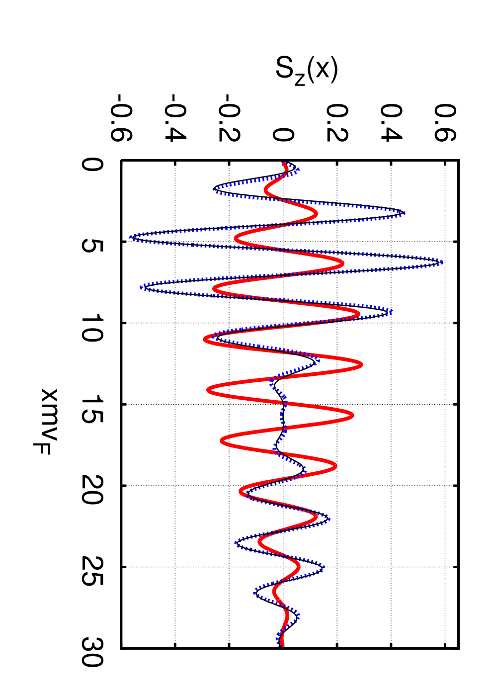
(2)

It is remarkable that the spin-orbit coupling constant enters via the period of beating only.

Net spin polarization. Consider a semi-infinite ballistic 2DEG described by the Hamiltonian

$\displaystyle H=\int d{\bf r}~\hat{\psi}^{\dagger}\left[-\frac{{\bm{\partial}}^{2}}{2m}-i\lambda(\hat{\sigma}_{x}\partial_{y}-\hat{\sigma}_{y}\partial_{x})+U(x)\right]\hat{\psi},$

(3)

where potential $U(x)$ ensures boundary confinement (see Fig. 1). For the sake of simplicity we present derivation for the case of ’Rashba’ spin-orbit interaction, though calculations for the ’Dresselhaus’ coupling Dress are completely analogous both. The system is attached to two ideal reflectionless leads injecting equilibrium electrons into 2DEG. The chemical potentials of the leads are shifted by the applied voltage, $eV$.

Since $k_{y}$ is an integral of motion (in case of reflectionless leads), it is convenient to use the Fourier representation along the $y$-axis for the electron operators, $\hat{\psi}({\bf r})=\sum_{k_{y}}\hat{c}_{k_{y}}(x)e^{ik_{y}y}$. One can now derive the equation of motion for the expectation value of the electron spin operator, ${\bf s}(k_{y},x)=\frac{1}{2}\langle\hat{c}^{\dagger}_{k_{y}}(x)\hat{\bm{\sigma}}\hat{c}_{k_{y}}(x)\rangle$, which can be readily written in the form,

$$\partial_{t}s_{y}(k_{y},x)=-\partial_{x}J^{y}_{x}(k_{y},x)-2\lambda k_{y}s_{z}(k_{y},x).$$

(4)

Here $J_{x}^{y}$ stands for the conventional operator of spin-current, i.e.,

$$J^{y}_{x}(k_{y},x)=\frac{i}{4m}\langle\nabla_{x}\hat{c}^{\dagger}_{k_{y}}\hat{\sigma}_{y}\hat{c}_{k_{y}}-\hat{c}^{\dagger}_{k_{y}}\hat{\sigma}_{y}\nabla_{x}\hat{c}_{k_{y}}\rangle-\frac{\lambda}{2}\langle\hat{c}^{\dagger}_{k_{y}}\hat{c}_{k_{y}}\rangle.$$

In a steady state the lhs of Eq. (4) vanishes. Integrating Eq. (4) over the $x$-direction, we obtain for the net spin polarization,

$$\int_{-\infty}^{\infty}s_{z}(x)dx=-\frac{1}{2\lambda}\sum_{k_{y}}\frac{1}{k_{y}}J^{y}_{x}(k_{y},\infty).$$

(5)

It is straightforward to calculate the value of the ($k_{y}$-resolved) spin current $J^{y}_{x}(k_{y},\infty)$ inside the bulk of a 2D system:

$$J^{y}_{x}(k_{y},\infty)=-\frac{1}{2}\sum_{\beta=\pm 1}\sum_{k_{x}}\left(\lambda+\frac{\beta k_{x}^{2}}{mk}\right)n_{\beta}(k_{x},k_{y}),$$

(6)

where $n_{\beta}(k_{x},k_{y})$ stands for the population of different momentum states in the subband $\beta$. Only “uncompensated” states contribute to the non-equilibrium spin polarization given by Eqs. (5-6); these states describe electrons that originate in the left lead ($k_{y}>0$) and belong to the energy interval near the Fermi energy, $E_{F}<k^{2}/2m+\beta k\lambda<E_{F}+eV$. The integral (5) diverges logarithmically at $k_{y}\to 0$. Assuming the same infrared cut-off in both subbands, $\widetilde{k}$, we observe that the diverging $\ln{\widetilde{k}}$-contributions in the two subbands cancel each other, yielding in the linear (in $V$) response,

$$\int_{-\infty}^{\infty}s_{z}dx=\frac{eV}{2\lambda(2\pi)^{2}}\left(\frac{2\lambda}{v_{F}}-\ln{\frac{v_{F}+\lambda}{v_{F}-\lambda}}\right)$$

(7)

where $v_{F}=\sqrt{2E_{F}/m+\lambda^{2}}$ is the Fermi velocity. Expanding this general result to the lowest non-vanishing order in $\lambda/v_{F}$ we recover the net boundary polarization, Eq. (1).

Evanescent modes. The reflection at the boundary mixes the two bulk subbands. Those states that belong to the domain, $k^{+}<k_{y}<k^{-}$, where $k^{\pm}=m(v_{F}\mp\lambda)$, refereed to as evanescent states usaj, are characterized by exponentially decaying contribution from the upper ($+$) subband. Repeating the calculations leading to Eq. (7) but now for the evanescent domain only, we obtain,

$$\int_{-\infty}^{\infty}s_{z}^{\text{ev}}dx=\frac{eV}{2\lambda(2\pi)^{2}}\left(2\sqrt{\frac{\lambda}{v_{F}}}-\ln{\frac{1+\sqrt{\lambda/v_{F}}}{1-\sqrt{\lambda/v_{F}}}}\right).$$

(8)

Remarkably, the net evanescent contribution is $\sim\sqrt{\lambda}$ and is largely canceled by the contribution from the normal domain $k_{y}<k^{+}$, yielding Eq. (1) which is quadratic in $\lambda$. This cancelation occurs for local spin density as well, see Eq. (2).

Electron Green’s function. Microscopic calculation of the local spin polarization can be most simply performed with the help of the electron Green’s functions,

$${\bf s}(x)=i\frac{eV}{4\pi}\text{Tr}\int\limits_{0}^{k^{-}}\frac{dk_{y}}{2\pi}[G^{R}_{k_{y}E_{F}}(x,x)-G^{A}_{k_{y}E_{F}}(x,x)]\hat{\bm{\sigma}},$$

(9)

where $G^{R}_{k_{y}E}(x,x^{\prime})$ is the retarded Green’s function. Its advanced counterpart satisfies the condition $G^{A}_{k_{y}E}(x,x^{\prime})=G^{R\dagger}_{k_{y}E}(x^{\prime},x)$. The summation over energy in Eq. (9) is performed over the narrow strip of width $eV$, similar to Eqs. (6-7).

To illustrate how spin polarization arises from the solution of the Schrödinger equation, let us solve the problem of a hard-wall boundary: $U(x)=0$, for $x>0$ and $U(x)=\infty$ for $x<0$. The case of a smooth boundary where electrons adiabatically follow semiclassical trajectories for spin-split subbands SM will be considered separately ZSM.

For a plane wave, $\sim e^{ik_{y}y}$, the equation for the Green’s functions for ($x,x^{\prime}>0$) is

$$\left[\frac{\partial^{2}_{x}}{2m}-\lambda(i\hat{\sigma}_{y}\partial_{x}+\hat{\sigma}_{x}k_{y})+E^{\prime}\right]\hat{G}(x,x^{\prime})=-\delta(x-x^{\prime}),$$

(10)

where the subscripts $k_{y}$ and $E$ are omitted for simplicity, and $E^{\prime}=E-{k_{y}^{2}}/{2m}$. The boundary condition for the impenetrable wall is $G(x,0)=G(0,x^{\prime})=0$. We solve the problem by first noting that the following function $\hat{\cal L}(x)$ satisfies both the homogeneous equation (10) and the boundary condition $\hat{\cal L}(0)=0$,

$$\hat{\cal L}(x)=\frac{1}{i\sum_{\beta}k^{\beta}}\sum_{\beta}\frac{k^{\beta}}{k_{x}^{\beta}}\left(e^{ik_{x}^{\beta}x}\hat{B}_{\beta}-e^{-ik_{x}^{\beta}x}\hat{B}_{\beta}^{*}\right),$$

(11)

here ^∗ stands for the simple complex (not Hermitian) conjugate; the sum is taken over both subbands, with the projection matrix for the subband $\beta$ defined as

$$B_{\beta}=\frac{1}{2}\left(1+\beta\frac{k_{y}}{k^{\beta}}\hat{\sigma}_{x}-\beta\frac{k_{x}^{\beta}}{k^{\beta}}\hat{\sigma}_{y}\right),$$

(12)

where the absolute value of the electron momentum $k^{\beta}$ is defined above Eq. (8) and its $x$-component is $k_{x}^{\beta}=\sqrt{(k^{\beta})^{2}-k_{y}^{2}}$. Here we concentrate on the normal modes, where both $k_{x}^{\pm}$ are real; rather simple modifications for the evanescent domain (where $k_{x}^{+}$ is imaginary) are outlined below.

Using the function (11) we can readily construct the solution for the inhomogeneous equation (10) which satisfies the boundary condition $G(0,x^{\prime})=0$,

$$\hat{G}(x,x^{\prime})=-2m[\hat{\cal L}(x)\hat{A}(x^{\prime})+\Theta(x-x^{\prime})\hat{\cal L}(x-x^{\prime})],$$

(13)

where $\hat{A}(x^{\prime})$ is yet unknown matrix. Since Green’s function has to obey both the boundary condition $G(x,0)=0$ and the equation conjugated to Eq. (10), the matrix $\hat{A}(x^{\prime})$ must be a homogeneous solution satisfying the condition $\hat{A}(0)=-1$. This determines it up to some constant matrix $\hat{C}$ different for the retarded and advanced Green’s functions, $\hat{A}(x^{\prime})=\hat{C}\hat{\cal L}^{\dagger}(x^{\prime})-\partial_{x^{\prime}}\hat{\cal L}^{\dagger}(x^{\prime})$,

	$\displaystyle\hat{G}_{R,A}(x,x^{\prime})$	$\displaystyle=$	$\displaystyle-2m\Bigl[\hat{\cal L}(x)\hat{C}_{R,A}\hat{\cal L}^{\dagger}(x^{\prime})-\hat{\cal L}(x)\partial_{x^{\prime}}\hat{\cal L}^{\dagger}(x^{\prime})$		(14)
			$\displaystyle+\Theta(x-x^{\prime})\hat{\cal L}(x-x^{\prime})\Bigr].$

The constant $\hat{C}_{R}$ ($\hat{C}_{A}$) is most simply determined from the condition that the retarded (advanced) Green’s function does not contain the waves $\sim e^{-ik_{x}^{\beta}x}$ ($e^{ik_{x}^{\beta}x}$) propagating to (from) the boundary in the region $x>x^{\prime}$. The calculations are straightforward but rather tedious. As a result one obtains,

	$\displaystyle\hat{C}_{R,A}=\mp\frac{i}{2}\left(k_{x}^{+}+k_{x}^{-}\right)\mp\frac{i}{2k_{y}}\left(k^{-}k_{x}^{+}-k^{+}k_{x}^{-}\right)\hat{\sigma}_{x}$
	$\displaystyle-im\lambda\hat{\sigma}_{y}+\frac{1}{2k_{y}}\left(k^{+}k^{-}-k_{y}^{2}-k_{x}^{+}k_{x}^{-}\right)\hat{\sigma}_{z},$		(15)

where the upper (lower) sign corresponds to $\hat{C}_{R}(\hat{C}_{A})$.

Spin polarization. Making use of the derived Green’s function we can now calculate the local spin polarization (9). With the help of Eqs. (14) and (Spin-Hall edge spin polarization in a ballistic 2D electron system) we obtain

	$\displaystyle s_{z}(x)=\frac{eV}{2(2\pi)^{2}mv_{F}^{2}}\left\{\int_{0}^{k^{+}}\frac{dk_{y}}{k_{y}}~(k^{+}k^{-}+k^{2}_{y}-k^{+}_{x}k^{-}_{x})\Big[\sin(2k^{+}_{x}x)+\sin(2k^{-}_{x}x)-2\sin((k^{+}_{x}+k^{-}_{x})x)\Big]\right.$
	$\displaystyle\left.-\int_{k^{+}}^{k^{-}}\frac{dk_{y}}{k_{y}}~\Big[k^{-}_{x}\kappa(e^{ik_{x}^{-}x}-e^{-\kappa x})^{2}-2(k^{+}k^{-}+k_{y}^{2}+ik_{x}^{-}\kappa)\sin(k^{-}_{x}x)(\cos(k^{-}_{x}x)-e^{-\kappa x})\Big]\right\}$		(16)

The first line here is the contribution of the normal modes while the second line comes from the evanescent modes, where $\kappa=\sqrt{k_{y}^{2}-(k^{+})^{2}}$ evanesc. By calculating the integral over $x$ it is straightforward to verify that the net contribution of the evanescent modes satisfies Eq. (8), being $\sim\sqrt{\lambda}$. This is mostly canceled by the contribution from the normal modes. The total net contribution of both the normal and evanescent states yields Eq. (7) in agreement with our general argument based on the equation of motion for spin operators, Eq. (4). Behavior of the local spin density (Spin-Hall edge spin polarization in a ballistic 2D electron system) is shown in Fig. 2. In the most relevant limit, $\lambda\ll v_{F}$, Eq. (Spin-Hall edge spin polarization in a ballistic 2D electron system) can be simplified to:

	$\displaystyle s_{z}(x)=-eV\frac{m\lambda}{\pi^{2}v_{F}}\int_{0}^{1}dy\sin({x}\sqrt{1-y}/\xi)e^{-x\sqrt{y}/\xi}$
	$\displaystyle+\frac{eV}{16\pi^{2}mv_{F}^{2}x^{2}}\sum_{\beta}~[\sin{(2k^{\beta}x)}-2k^{\beta}x\cos{(2k^{\beta}x)]}$
	$\displaystyle-\frac{eV(k^{+})^{2}}{4\pi^{2}mv_{F}^{2}}\int_{0}^{1}dy~\sin[xk^{+}(\sqrt{y}+\sqrt{\delta+y})],$		(17)

where $\xi^{-1}=2m\sqrt{\lambda v_{F}}$, and $\delta=(k^{-}/k^{+})^{2}-1$. Integrating this expression over $x$ we recover the net spin polarization (1).

Spectral distribution of spin density. It is instructive to present the results in terms of the Fourier transform of the spin density, $s_{z}(q)=2\int_{0}^{\infty}dxs_{z}(x)\sin{qx}$. From Eq. (Spin-Hall edge spin polarization in a ballistic 2D electron system) we find $s_{z}(q)$ in a form of piecewise continuous algebraic function defined in four domains. The surprising feature of the spectral distribution revealed by this calculation is its vanishing, $s_{z}(q)=0$, in the whole long-wavelength domain, $0<q<2k^{+}$. In particular, this shows the exact cancelation between normal and evanescent modes. For larger values of $q$ we obtain to the leading order in $\lambda$,

$$s_{z}(q)=\frac{eVq}{16\pi mv_{F}^{2}}\left\{\begin{array}[]{cl}-1,&2k^{+}<q<2mv_{F},\\ 1,&2mv_{F}<q<2k^{-},\\ -2/(q\xi)^{4},&2k^{-}<q.\end{array}\right.$$

(18)

The plot of the spectral distribution is illustrated in Fig. 3. Remarkably, the net spin polarization (given by $\pi^{-1}\int dqs_{z}(q)/q$) comes from the large-$q$ tail ($\propto q^{-3}$) in the spectral density $s_{z}(q)$.

Conclusion. In this paper we solved analytically a problem of mesoscopic spin-Hall effect in a confined 2D electron system. We presented general arguments why the net spin polarization in a ballistic spin-Hall effect is independent of the boundary potential and confirmed the result by a straightforward calculation for the hard-wall boundary, for which the analytical solution was obtained. The spectral distribution of spin density consists of two narrow peaks of opposite sign whose heights are virtually independent of the small spin-orbit coupling constant. Surprisingly, long-wavelength contributions from evanescent and normal modes exactly cancel each other. Understanding the level of universality of this result for arbitrary boundary potentials remains a challenging problem.

We acknowledge fruitful discussions with A. Andreev, B. Halperin, M. Raikh and O. Starykh. The work was supported by DOE, Award No. DE-FG02-06ER46313 and by SFB TR 12.

References

- (1) M.I. Dyakonov, V.I. Perel, Phys. Lett. A 35, 459 (1971).
- (2) Y.K. Kato et. al, Science 306, 1910 (2004); V. Sih et. al, Nature Physics 1, 31 (2005).
- (3) J. Wunderlich et. al, Phys. Rev. Lett. 94, 047204 (2005).
- (4) S.O. Valenzuela and M. Tinkham, Nature 442, 176 (2006).
- (5) J.E. Hirsch, Phys. Rev. Lett. 83, 1834 (1999).
- (6) Shufeng Zhang, Phys. Rev. Lett. 85, 393 (2000).
- (7) H.A. Engel, B.I. Halperin, and E.I. Rashba, Phys. Rev. Lett. 95, 166605 (2005).
- (8) W.-K. Tse, S. Das Sarma, Phys. Rev. Lett. 96, 056601 (2006).
- (9) S. Murakami, N. Nagaosa, and S.-C. Zhang, Science 301, 1348 (2003).
- (10) J. Sinova et. al, Phys. Rev. Lett. 92, 126603 (2004).
- (11) S. Murakami, Adv. in Solid State Phys. 45, 197 (2005), cond-mat/0504353; H.A. Engel, E.I. Rashba, and B.I. Halperin, cond-mat/0603306.
- (12) E. G. Mishchenko, A. V. Shytov, and B. I. Halperin, Phys. Rev. Lett. 93, 226602 (2004).
- (13) A. A. Burkov, A. S. Núez, and A. H. MacDonald, Phys. Rev. B 70, 155308 (2004).
- (14) A.G. Mal’shukov et. al, Phys. Rev. Lett. 95, 146601 (2005).
- (15) I. Adagideli and G. E. W. Bauer, Phys. Rev. Lett. 95, 256602 (2005).
- (16) V. M. Galitski, A. A. Burkov, and S. Das Sarma, Phys. Rev. B 74, 115331 (2006).
- (17) O. Bleibaum, Phys. Rev. B 74, 113309 (2006).
- (18) Ya. Tserkovnyak et. al, cond-mat/0610190.
- (19) R. Raimondi et. al, cond-mat/0701629.
- (20) K. Nomura et. al, Phys. Rev. B 72, 245330 (2005).
- (21) B.K. Nikolic et. al, Phys. Rev. B 72, 075361 (2005); Phys. Rev. Lett. 95, 046601 (2005); E.M. Hankiewicz et. al, Phys. Rev. B 70, 241301(R) (2004).
- (22) S. Datta, Electronic Transport in Mesoscopic Systems, (Cambridge University Press, 1995).
- (23) G. Usaj and C.A. Balseiro, Europhys. Lett. 72, 621 (2005); A. Reynoso, G. Usaj and C.A. Balseiro, Phys. Rev. B 73, 115342 (2006).
- (24) T.D. Stanescu and V. Galitski, Phys. Rev. B 74, 205331 (2006).
- (25) V. Sih et. al, Phys. Rev. Lett. 97, 096605 (2006).
- (26) S.I. Erlingsson et. al, Phys. Stat. Sol. C 3, 4317 (2006).
- (27) Yu.A. Bychkov and E.I. Rashba, J. Phys. C 17 6039 (1984).
- (28) G. Dresselhaus, Phys. Rev. 100, 580 (1955).
- (29) When both Rashba and linear Dresselhaus () couplings are present the methods developed in this Letter are still fully applicable. In particular, the expression (1) is valid provided that we change, .
- (30) P.G. Silvestrov and E.G. Mishchenko, Phys. Rev. B 74, 165301 (2006).
- (31) V.A. Zyuzin, P.G. Silvestrov, and E.G. Mishchenko, in preparation.
- (32) To obtain the Green’s function in the evanescent domain () one has to substitute into , Eq. (12), and use the Hermitian conjugate instead of in Eq. (11). In addition, vanishing of exponentially growing terms requires the substitution () to be made in (), see Eq. (Spin-Hall edge spin polarization in a ballistic 2D electron system).