Study in a beam test of the resolution of a Micromegas TPC with standard readout pads
Abstract
The results of a beam test performed at the KEK PS in June 2005 are presented. Drift properties of an argon-isobutane mixture have been accurately measured and compared with predictions at magnetic fields between 0 and 1 Tesla. The r.m.s. point resolution of a padrow is compared with simulation and with an analytical calculation. The fundamental limitations due to detector geometry and gas properties are reviewed and the measured performances of the detector are found to be close to this limit. A numerical application to the case of a Linear Collider TPC is presented.
1 Introduction
Three of the four detector concepts which have been proposed for the Linear Collider foresee a large Time Projection Chamber (TPC) as a main tracker. This allows continuous tracking to be performed, yet with a minimal amount of matter. Depending on the detailed designs, the TPC should have about 200 padrows with a space resolution between 100 and 150 microns in the R direction. Mainly three technologies are currently considered for the gas amplification in these TPCs : a Multi-Wire Proportionnal Chamber (MWPC), a Micromegas chamber, and a multiGEM structure. To this end, R&D has been pursued since the beginning of the decade within the LC-TPC collaboration[1] and has lead to the construction of several prototypes. It was felt useful to gather around a single experiment and to have a way of comparing the various technologies in a well-defined framework, with the same readout electronics and chamber geometry. This is the purpose of the Asian-Canadian-European Multi-Prototype collaboration. It started with the construction of a MWPC chamber in MPI Munich, which took beam data at KEK in April 2004. Then the chamber was equipped with a triple-GEM structure and took beam data in April 2005. This paper reports on a beam test carried out with a Micromegas endplate in June 2005.
The detector and the operation conditions are described in Section 2, where an assessment of data quality is given. The results on gas properties (drift velocity, diffusion) are presented in Section 3. Section 4 is devoted to the spatial resolution of the device. It starts with a theory elaborated in our group which is then compared to simulations and measurements. Fundamental limitations from the gas mixture and pad geometry are assessed and consequences for a Linear Collider TPC are drawn.
2 Experimental Setup and Data Taking
This experiment was carried out using the beam line at the KEK 12 GeV PS. The beam line provided a secondary beam of pions or protons with momenta up to 4 GeV/c through the interaction of 12 GeV protons on a Be target, followed by the charge and momentum selection with a set of dipole magnets. The beam spill has a flat top of s with a repetition rate of Hz. There were 4 scintillation counters, TC1 through TC4, whose 4-fold coincidence triggered the data acquisition on 4 GeV negatively charged pions. A typical trigger rate was Hz. The first two trigger counters, TC1 and TC2, were placed at the entrance of the beam just downstream of a beam slit to control the beam intensity and had an overlap region of cm2. The other two trigger counters, TC3 and TC4, were located at 8 m downstream of TC1 and TC2, that is, just in front of our Multi-Prototype TPC (MP-TPC). TC3 and TC4 had an overlap region of cm2 that matched the drift region of the chamber. The MP-TPC together with TC3 and TC411 1 TC3 and TC4 were equipped with fine-mesh photo multipliers, Hamamatsu R6682, which allowed operation in a magnetic field up to 1 Tesla. were installed in a Persistent Current solenoidal Magnet (PCMAG) having a bore diameter of cm and a length of m with a very thin wall of % radiation lengths. The magnet capable of creating a field up to 1.2 Tesla was operated in the closed loop mode and provided a field uniformity better than % in the drift region of the MP-TPC that was aligned with the magnet axis, so that the electric drift field was parallel to the magnetic field.
In the following, unless otherwise stated, the beam was shot perpendicular to the drift axis of the MP-TPC. The nominal size of the beam in these conditions is about 4 cm at the chamber. To cover the whole active volume of the MP-TPC, we hence spread the beam by inserting a 5 cm-thick lead brick just downstream of TC1 and TC2 in the normal data taking conditions.
2.1 Multi-prototype TPC
The MP-TPC has a cylindrical drift region of 261 mm in length and 145 mm in diameter. As seen in Fig. 1,

the field cage is made of fourteen 15 mm-wide circular rings spaced 3.2 mm apart and a cathode disk with a small hole at its center22 2 The hole lets X-rays from an 55Fe source enter the drift volume, for gain calibration and monitoring purposes. . All of these are embedded into a gas-tight vessel, which is closed on one side by a detachable endplate detector that carries a Micromegas foil and readout pads. The ring closest to the Micromegas detector is at a distance of 6 mm from the mesh.
The Micromegas endplate, built in Saclay and Orsay, consists of a 0.8 mm thick Printed Circuit Board bearing anode pads, with a mesh stretched on a frame and mounted above the pad plane. The mesh is m thick Cu having circular holes of m in diameter placed with a m pitch. The mm2 frame leaves a mm2 active area. A 50-micron gap is maintained between the mesh and the pad plane by kapton pillars. In normal operation a voltage of about 350 V is applied to the mesh relative to the pad plane at 0 V. The resulting electrostatic force sticks the mesh to the anode plane. There are 12 rows of 32 pads on the anode plane. Each pad has a rectangular shape and is placed at a pitch of 6.3 mm along the beam ( direction) and 2.3 mm transverse to the beam ( direction).
The chamber is filled with an argon mixture containing 5% isobutane and is operated at room temperature and at atmospheric pressure.
2.2 Readout Electronics and DAQ
The 12 rows of 32 readout pads (384 in total) are connected via cm long flat cables to 24 ALEPH preamplifiers[2], each having 16 channels and reading out a half of a pad row. The shaped signals from the preamplifiers are sent to ALEPH TPDs (TPC Digitizers) in a Fastbus crate via m long twisted pair cables and are sampled at a rate of 12.5 MHz and digitized over 8 bits. The data are then read out, via a Fastbus-VSB translator unit, , by a VME board computer, , operating on OS/2. The readout data are stored via TCP/IP connection on a Linux PC in the LCIO format[3]. The data acquisition time is about s per event, which limited the data acquisition speed to about event per spill.
2.3 Data Taking
A typical event taken at a magnetic field of 0.5 T is shown in Fig. 2.

During the data taking, the gain was continuously monitored by a 55Fe source. The mesh signal was readout by a fast charge amplifier ORTEC 142B and the signal was sampled with an AMPTEK Multi-Channel Analyser MCA8000. A spectrum obtained this way is shown in Fig. 3 where the 5.9 keV line and the escape line in argon are seen. The source was not collimated. The Landau distribution of the ionisation produced by the 4 GeV pions from the beam is also visible and peaks at 12.5 keV as expected for the 75 mm active length of gas. Over a period of 60 hours the extreme variations of gain were 3% and the r.m.s. gain variations were 3 per mil over this period.

The gain is measured as a function of the mesh voltage (Fig. 4). The data presented here were taken at a mesh voltage of 320 V, corresponding to a gain of 3650, in a magnetic field of 0.5 and T, and a mesh voltage of 340 V (gain of 7500) for the data taken with no magnetic field.

A total of 4020 triggers were collected at T, 6111 at T and 5166 at T. The temperature was 28 to 32 ∘C during the data taking. The gas pressure in the vessel followed the atmospheric pressure which was stable during the runs used in this paper.
In the following analyses, the first two and last two padrows, as well as the four leftmost and two rightmost pads of each row, are not used in the measurements, to avoid edge effects. However, when a hit is found close to the edges of this fiducial region, the neighbouring pad(s) in the region are recovered and used in the track reconstruction.
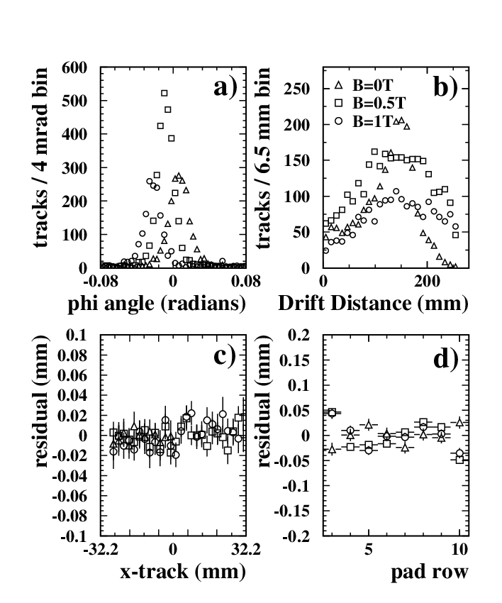
The azimuthal angle distribution is shown in Fig. 5a. As stated earlier a wide beam was obtained by adding a cm-thick lead brick in the beam line. The resulting distribution of the tracks is shown in Fig. 5b. The uniformity of the detector can be assessed from the average residual vs track position in (Fig. 5c) and vs padrow number Fig. 5d for the 8 fiducial padrows. Distortions up to 50 microns are observed at non-zero magnetic field (likely to be due to effects), but they do not affect the resolution measurements where only the r.m.s. of the residuals is considered.
2.4 Data Analyses
The exactly same data sample has been analysed with two independent analysis methods and compared in the following. They differ primarily by the way the track parameters are fitted to the pad data in the - plane. The geometrical track parameters are the intercept of the track with the axis (), the azimuth at this point (), and the inverse radius of curvature .
In the first method, a global maximum-likelihood fit of the geometrical track parameters, together with the track width () to the charge of the pads is carried out[4]. In other words, a track is represented by an arc of a circle with a gaussian charge spread of width along the direction, and is an additional fit parameter. The pad charge and time are determined as follows: the ADC counts of the 3 preceding and 3 following the time bucket where the maximum is reached are added together with the bucket of maximum charge. This sum is required to exceed a minimum of 7 ADC counts for the pad to be included in a hit. The time associated to the hit pad is the charge-weighted average of the seven buckets used in the charge integration.
The log-likelihood function which is maximised with respect to the 4 track parameters reads: , where is the fraction of the charge expected in pad , obtained by integration over the pad of a function with a gaussian profile transverse to the track. is the number of electrons before amplification corresponding to the charge readout on the pad . This method is implemented in the FORTRAN 95 program FTPC[5].
In the second method, a fit is performed to hit points on a row-by-row basis. The method is implemented in C++ and available as the Double-Fit program[6]. The Double-fit program starts with cluster finding in the plane of pad-number vs time-bucket for each pad row. To build a 2-dimensional ( and ) cluster, consecutive time buckets are summed, starting from the first pulse encountered above ADC counts, up to the first below 6 counts. Such a hit is accepted if its peak pulse height exceeds ADC counts. The coordinates of the hit is then calculated as its charge barycenter. Following the cluster finding, the program then performs a fit of either a straight line at or a circle at or T.
3 Gas Properties
3.1 Drift Velocity Measurements
Measuring the drift velocity of gas mixtures is an interesting test of the electron transport simulation in gases, or alternatively can be considered as a check of gas purity and composition. The drift field was set to 220 V/cm and the detector was taken outside the magnet, itself not energized. For this measurement a novel and very simple technique was used: the beam was shot at an angle of 45 degrees to the center of the cathode. A cm2 scintillator was added in the trigger to select pions crossing the cathode plane in the center. Electrons from ionisation close to the cathode drift all the way along the axis of the TPC reaching the central pads of the detector, in the region where no electric-field distortions are expected. The TPD measures the time elapsed between the trigger arrival and the signal arrival. The end-point of this time distribution, added to the delay between the trigger and the readout, is the time taken by the electrons to drift along the 260.8 mm chamber. The drift time is found to be . The trigger delay was measured to be . Adding a rough estimate of for the NIM to ECL converter at the entrance of the TPD, and subtracting an estimated ns for the pad signal delay in the m readout cables, the total drift time is measured to be . Dividing the chamber length by this time yields . An alternative method has also been used, with a wide beam perpendicular to the axis of the chamber and also measuring the endpoint of the time distribution. It leads to the value of , in agreement with the former. These two values are combined assuming fully correlated systematics to yield the measurement of the drift velocity of electrons in Ar+5% isobutane mixture at an electric field of 220 V/cm of
This value is used for the determination of the coordinate of the hits along the axis of the chamber in the following data analyses.
This measurement is in very good agreement with the Magboltz[7] prediction of . The uncertainty on the prediction is dominated by the error on the gas composition, stemming from a 2% uncertainty on the isobutane gas flow. No consideration on the model, the approximations nor on the input data used in the simulation enter this estimate of the prediction uncertainty.
3.2 Transverse Diffusion Constant Measurements
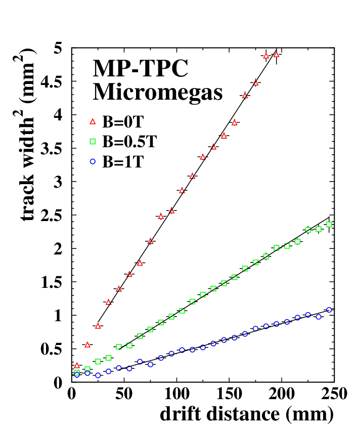
For large enough drift distances, so that the ionisation charge is spread over several pads, the width of the track allows the determination of the diffusion constant using the relation .
In the global likelihood method, is obtained by maximising the track likelihood simultaneously for the geometrical track parameters. Fig. 6 shows for the 3 values of the magnetic field the relation between the average and the drift distance . The expected linear dependence on the drift distance , for large , is clearly seen. The data at low , where the sensitivity to is lost and where the spread in track widths is comparable to the average track width, are not included into the linear fit. The slight offset in the case of zero magnetic field, corresponding to 0.3 mm added in quadrature to the track width, can probably be attributed to delta rays. At higher fields the path of these delta-ray electrons are expected to be limited by the magnetic field. The fitted values are given in the first line of Table 1. The quoted uncertainties include systematics from the noise level and threshold used to reconstruct the hits.
In the second method, the average fraction of the charge falling on a given pad is plotted as a function of the distance between the track and the pad center. It can be shown (see Appendix A) that for large enough drift distances and for high enough magnetic fields to curl up delta-ray electrons, this distribution becomes gaussian and its width scales as , where is the pad pitch. The measured values of by this method are shown in the second line of the table. These two measurements are in good agreement with each other and with the Magboltz prediction, at the level of a few percent.
| Magnetic field | 0 T | 0.5 T | 1 T |
| Global likelihood | |||
| method | |||
| Magboltz | 469.3 | 284.1 | 192.6 |
4 Resolution
4.1 Theory and Simulation
4.1.1 Effective Number of Ionisation Electrons
In this section, we present an analytic formula for the spatial resolution of a TPC equipped with a readout plane consisting of a gaseous detector that amplifies track electrons and rows of readout pads to measure their charge centroids. For simplicity, consider a charged particle passing through the TPC at the right angle to a pad row and at a drift distance from the readout plane. In this zero crossing angle case, as far as the size of the primary ionisation clusters is negligible33 3 This assumption is justifiable at high magnetic field which is expected to curl up delta rays and hence suppress the size of the primary ionisation clusters. , all of the track electrons created in the ionisation will have a -function-like distribution peaking at, say, , when projected onto the -axis, namely, the axis in the pad row direction.
These track electrons drift toward the pad row. While drifting, each of these track electrons experiences transverse diffusion and will have an -coordinate deviated from by , i.e. , according to the probability distribution:
| (1) |
where the subscript, , means -th electron and with being the transverse diffusion constant.
The number of track electrons that will reach the gas amplification region in front of the pad row fluctuates statistically. Let us denote the probability of getting such ionisation electrons eventually contributing to the signal induced on the pad row by with being the average: .
Each of these ionisation electrons will be gas-amplified at the readout plane by a factor, , which is assumed here to fluctuate according to a Polya distribution:
| (2) |
with being the average gas gain: . Notice that the Polya distribution becomes exponential in the limit, while it coincides a -function in the limit. Notice also that the Polya distribution has a variance: , which goes to zero as as expected.
For illustration purpose, let us assume, for a while, an idealistic readout plane which measures the -locations of individual electrons with infinite accuracy but with relative weights of gas gain values. Then, the center of gravity of these electrons at the readout plane will be given by
| (3) |
The charge centroid, , will then be distributed according to
| (5) | |||||
Under the assumption that is large enough and hence
| (6) |
we obtain the variance of the center of gravity, , by inserting Eqs.(3) and (5) into its definition and carrying out the integral:
| (7) | |||||
| (8) |
where use has been made of
| (9) |
and
| (10) |
The is hence given by
| (11) |
Notice that is in general significantly smaller than due
to ionisation statistics.
The gain fluctuation further reduces [9]
by as much as a factor of two for the exponential gain fluctuation: .
In order to find a lower limit on , let us consider the total charge distribution. The total charge after gas amplification is given by
| (12) |
and then its probability distribution function by
| (13) |
From this we can readily obtain the variation of the total charge as
| (14) | |||||
| (15) |
This implies that in the case of a Landau-like , for which , the gas gain fluctuation will not affect the total charge distribution very much.
For X-rays from , however, we expect
| (16) | |||||
| (17) |
where the Fano factor is about 0.2 and is about 220 for argon. The best resolution so far attained with a Micromegas detector with exactly the same type of mesh is about 6.8% in r.m.s.[8], which implies . This is a lower limit in the sense that it neglects experimental effects increasing the width, other than gas gain fluctuations (electronic noise for instance). However, can be smaller if the Fano factor is less than 0.2. Taking a value , still consistent with measurements and theoretical calculations [10], would lead to a minimum value of 0.166 for .
4.1.2 Effects of Finite Size Pads
In the last section, we considered gain fluctuation in the gas amplification process at the end plane detector but assumed that we could measure the location of a single electron with infinite accuracy. We now introduce a pad row of pitch to measure the charge centroid:
| (18) |
where is the charge on pad and is given as the sum of contributions from seed electrons:
| (19) |
with being the response function of pad for seed electron arriving at the location and being the electronic noise on pad . Notice that the pad response function is normalized as
| (20) |
The probability distribution for is then given by
| (22) | |||||
where represents a constant electronic noise with and . On the other hand, the probability distribution for the charge centroid is given by
| (25) | |||||
which replaces Eq.(5).
Since the probability distribution depends on the true location of the seed cluster , we average over to define :
| (26) |
Substituting Eq.(25) in this, and performing integration over , , and in this order, and then averaging over , we obtain
| (29) | |||||
where we have ignored the electronic noise as compared to the total charge:
and
as usual.
Notice that the pad response function only appears in the following two forms:
| (30) |
and
| (31) |
and can be numerically evaluated, once the functional form of is given.
The formula, Eq.(29), can be qualitatively interpreted as follows. The first term is the mean square of the difference between the charge centroid and the true location of the seed cluster and is independent of the number of primary electrons44 4 It is well known that there is an -shape systematics in the difference between the simple charge centroid and the true cluster location. This term can hence be eliminated by correcting the charge centroid for the -shape systematics. . This term vanishes in the narrow pad limit, , while it approaches the famous in the wide pad limit, . The second can be interpreted as the combined effect of the diffusion and the gas gain fluctuation. As we have seen in the previous sections, their contributions scale as . The last term represents the contribution from the electronic noise and is independent of the shape of the pad response function or the diffusion. It scales as .
4.1.3 Application to a Micromegas-like Readout Plane
The qualitative observations we made in the last section agree with naive expectations. For quantitative comparison with data, however, we need a concrete form of the pad response function. For simplicity, let us assume that the spatial size of the avalanche caused by a single seed electron is negligible compared to the pad width, as expected for a Micromegas-like readout plane. In this limit, the pad response function becomes hodoscope-like:
| (32) |
for which we have
| (33) |
Substituting these in Eq.(29), we obtain
| (36) | |||||
As long as as at long distance, in the integrand of the above equation the first term can be ignored and the second term can be approximated (see Appendix B) by
| (37) |
In this long drift distance limit, we have an asymptotic formula:
| (38) |
which implies
| (39) |
if the electronic noise is negligible.
The integration in Eq.(36) can be carried out numerically at any drift distance, using
| (40) | |||||
| (41) | |||||
| (42) |
This and Eq.(36) imply that is a function only of and . Fig. 7 plots as a function of this scaling variable, .
Notice that the full theory curve merges into the asymptotic formula at around , which means that the effect of finite pad pitch becomes negligible for . The full theory has a fixed point, , at , while the asymptotic formula scales as . The full theory curve attains its minimum of about at around .
4.1.4 Comparison with Monte Carlo Simulation
A Monte-Carlo simulation has been carried out to check the analytical theory and to estimate the expected effective number of electrons for the gas mixture used in the tests.
In a first step track segments are generated with a uniform distribution of across a 2.3 mm pad and for a set of values along the drift axis. The number of ionisation clusters is generated along a 6.3 mm pad according to a Poisson distribution with mean value 32.0. This average number of clusters is estimated as follows: a concentration-weighted average of the number of clusters from minimum ionizing particles (m.i.p.) in Ar (23 e-/cm) and in isobutane (84 e-/cm), taken from ref. [11], multiplied by the calculated ratio of ionisation for 4 GeV pions with respect to m.i.p., taken to be 1.23 from ref. [12]. In each cluster a number of electrons is generated according to the argon cluster size distribution given in ref. [13]. The average is predicted to be 1/38.7.
Then each individual electron is transported over the distance . The transverse diffusion in the direction is simulated by varying by a random amount, following a gaussian law, the width of which is given by , where is the Magboltz prediction for the diffusion constant : , and mm/ for , and T, respectively.
The last step is to simulate the gas amplification gain. For this a Polya distribution with the parameter equal to 0.22 is used. For every track, the charge sum on each pad is calculated. Then hits are reconstructed as barycentres of the pads hit. The resolution for each is plotted in Fig. 8. The analytical formula, with input , as given by Eq. 11, reproduces the Monte Carlo data very well.
4.2 Comparison with Measurements
In the global likelihood analysis, the hit position on each row is estimated by a fit to the charge depositions in the row, with the track parameters fixed to their value using the 8 fiducial rows. The resolution is then calculated as the geometric mean of the r.m.s. values of the distributions of the residuals with and without the pad row in question in the fit (see Appendix C) so as to eliminate contributions from the tracking errors. To avoid being sensitive to outliers (produced by noise for instance) the hits situated at a distance of more than 4 standard deviations from the track are ignored. Alternatively, a gaussian function was fitted to the whole residual distribution to estimate its r.m.s.. This second estimate of the resolution is lower than the former by only 7%. The resolutions at and T are shown as a function of the drift distance in Figs. 9a), b), and c), respectively. The results of the global likelihood method are the triangles. The method results are also shown (square data points). The two methods agree each other very well at long drift distances. The discrepancies at short distances will be discussed later. The likelihood method makes a better use of the pad signal information.
These measured resolutions are compared with the theoretical predictions explained in the previous section, with . The fit using the barycentre of each row leads to values of consistent with this (see Table 2). The theory reproduces the data very well when as expected for and T. The theory seems to underestimate the resolution even at longer distances at and the discrepancy seems independent of the drift distance. This discrepancy could be attributed to the finite geometrical size of primary ionisation clusters that would be significant only when the curling up effect of delta-ray electrons is absent.
The hollow data points at small drift distance are not used in the fit. The reason to discard them is that they are biased toward low values, as the hits are reconstructed towards the middle of the pads. An example of this is given in Fig. 10, where the distribution of the position of hits with respect to the middle of a pad is shown; it is clear from this plot that for too small drift distance the hits are preferentially reconstructed in the middle of a pad, so that the whole track is biased towards the middle of the pad and the residuals are underestimated. This is the main reason why the rise of the resolution at low is underestimated in the data (this effect is less prominent in the case of T where the track curvature in the magnetic field plays the role of an effective pad staggering). This effect is present in both methods and could be avoided only if we had had an external measurement of the track position. Notice, however, that unlike the method which uses the charge barycentres, the likelihood method is free from the -shape systematics (the first term in Eq. 29) as long as each pad row has multiple pads above threshold. This is why the likelihood method tends to deviate from the theory and give better resolutions than the method in the short drift distance region.
The fitted values of are given in Table 2. Considering that is independent of the magnetic field, the 3 data sets can be combined to obtain a measurement of . This value can be compared with the expectation obtained in the previous section fixing the gain fluctuation parameter to 0.22, where the error is evaluated by varying all the other input parameters within their admissible range and adding in quadrature the variations of . The agreement is good, and favors significant gas gain fluctuations.
As explained in the previous section, a non-zero value of is expected from the fit to the data points of the functional form
The combined measurement of is , in good agreement with the expectation .
| Magnetic field | 0 T | 0.5 T | 1 T |
|---|---|---|---|
| Global likelihood | |||
| fit + barycentre |


4.3 Extrapolation to ILC-TPC
Conforted that the theory of resolution presented here is a pertinent approximation for a Micromegas TPC, we can use it to predict what can be expected in the 4 Tesla case, as proposed for the Linear Collider TPC. Fig. 11 represents the expected resolution as a function of , for two values of the pitch for the gas studied in this paper. One can see that at such a high magnetic field, the diffusion, with a constant of 63 m/, is not sufficient to spread the charge enough. This results in the fact that the hodoscope effect is felt up to distances over one meter in the case of a 2.3 mm pitch. Even a 1 mm pitch, which would require a very dense readout electronics and would feature pads with a large aspect ratio, would not allow the target average resolution of 100 m to be reached.
In the case of the triple mixture Ar:isobutane:CF4 (95:2:3), with a record diffusion constant as low as 26 m/, the situation is even more catastrophic: the hodoscope effect is felt over all distances even with 1 mm pads (Fig. 12).
This study shows that, to obtain the target resolution required to fulfill the ILC physics program, either smaller, digital pads are necessary, or a spreading of the charge onto several pads has to be implemented after amplification. The latter can be achieved either in a multi-GEM structure by maximizing the natural defocusing in the transfer between two GEMs, or by the use of a resistive-capacitive continuous layer (resistive foil) as proposed by some of us [14].


5 Conclusions
Successful operation of a Micromegas TPC in a test beam enabled us to measure its spatial resolution under a magnetic field as well as the properties of an Ar isobutane mixture. The drift velocity and the transverse diffusion constant for at and T are found to be in good agreement with the predictions of Magboltz. The obtained spatial resolution as a function of drift distance is well reproduced by an analytical calculation developed in this paper. The effective number of electrons is measured to be , which is consistent with an estimate based on the primary ionisation statistics and the gas gain fluctuations.
The extrapolation to the conditions of the Linear Collider shows that the goal resolution of 100 microns cannot be reached with mm pads with the technique used in this test, and that another technique will probably be necessary (digital smaller pad readout or resistive anode readout, for instance).
Acknowledgments
We would like to thank J. Pouthas for his kind support. We recognize D. Karlen for his help in using his JTPC display program and M.E. Janssen for his Doublefit analysis program. External institutes wish to thank the KEK directorate for the hospitality extended to them during the beam tests. We also thank the Cryomagnetism department for the operation of the magnets.
Appendix A Pad Response Function in the Large limit
From Eqs. (19) and (22) we obtain the average charge on pad :
resulting in the average charge fraction on pad :
| (43) | |||||
| (44) |
In our standard pad response function analysis, we plot this as a function of the pad center as measured from the average charge centroid:
| (45) | |||||
In the large limit, the charge fraction hence has the following functional form:
| (46) |
Since is apparently normalized to unity, we have
| (47) | |||||
| (48) |
and, consequently,
| (49) |
Appendix B Scaling and Limit
As long as the avalanche can be regarded as point-like, and the pad response function is hodoscope-like as given by Eq.(32), any observable with the dimension of length should scale as times a function of or times a function of . In the case of the first term of Eq.(36), it should hence scale as
| (50) |
where the pad pitch () can only appear in the function through the ratio: . This term represents the well known -shape systematic bias in the charge centroid for a finite pad pitch and will vanish in the limit: . It is, however, non-trivial whether this will vanish in the limit for a fixed pad pitch: . We can show analytically that this is indeed the case, as follows:
| (51) | |||||
| (52) | |||||
| (53) | |||||
| (54) |
where we have used the fact that is an even function of .
Noting that and hence in the large limit, we can further the calculation by Taylor expansion:
| (55) | |||||
| (56) | |||||
| (57) | |||||
| (58) | |||||
| (59) | |||||
| (60) | |||||
| (61) |
In order to see the large limit of the second and the third terms of Eq.(36), we need to evaluate the following:
| (62) | |||||
| (63) | |||||
| (64) | |||||
| (66) | |||||
| (68) | |||||
| (69) | |||||
| (70) | |||||
| (71) | |||||
| (72) |
where use has been made of Taylor expansion to the first order of :
| (73) | |||||
and the fact that the odd functions of vanishes upon integration and . Substituting the right hand side of Eq.(62) in Eq.(62) iteratively and ignoring the terms of , we finally arrive at
| (74) |
Notice that -independent term can be regarded as proportional to , and hence is no exception for the scaling law.
Appendix C Geometric Mean Method
In this appendix we give a simple demonstration of the geometric mean method applied in the analysis to estimate the spatial resolution.
First, in the case where the hit point in question (say, the -th point ) is excluded in the track fitting, the residual is given by
where represents the estimator for the -th point given by the track fitting using the remaining hit points. Its variance is
| (75) |
the sum of the true spatial resolution and the tracking error.
Next, in the case where the hit point in question is included in the track fitting, the estimator for the -th hit point is given by the weighted mean of and :
with being the corresponding weight: . The residual is hence given by
The variance of the residual in this case is therefore
| (76) |
References
- [1] http://www.mppmu.mpg.de/˜settles/tpc/welcome3.html
- [2] ALEPH Collaboration, TPC Manual.
- [3] http://lcio.desy.de/.
- [4] D. Karlen et al., Nucl. Instr. and Meth. A 555 (2005) 80.
- [5] K. Sachs, http://www.physics.carleton.ca/ gmd/FTPC/.
- [6]
M. E. Janssen, ’Auflösungsstudien an einer Zeit-Projektions-Kammer (TPC) mit GEM-Gasverstärkungssystem’,
Diplomarbeit, September 2004, Universität Dortmund, Germany, DESY-THESIS-2004-049.
R. Diener, ’Study of Reconstruction Methods for a Time Projection Chamber with GEM Gas Amplification System’, Diplomarbeit, Universität Hamburg, Germany,May 2006. - [7] ylonte Carlo simulation of electron drift and diffusion in counting gases under the influence of electric and magnetic fieldsy(TM) S. F. Biagi, Nucl. Instr. and Meth. A 421 (1999) 234.
- [8] P. Colas, ’New developments of Micromegas detectors for High Energy Physics’, in Proc. of the 32rd International Conference on High Energy Physics, Vol. I, p. 976, August 2004, Beijing, dapnia 04-348.
- [9] M. Kobayashi, Nucl. Instrum and Methods A 562 (2006) 136.
- [10] S. Biagi, talk given at the second TPC Jamboree (Aachen, 2007), http://www.physik.rwth-aachen.de/˜roth/jamboree-tpc/
- [11] B. Schmidt and K. Martens, ’Helium molecular gas mixtures for high resolution drift chambers’, Nucl. Instr. and Meth. A317 (1992) 148, and references therein.
- [12] E. Santovetti and L. Cerrito, ’Primary ionization and energy loss calculation for helium, neon, argon and krypton’, Nucl. Instr. and Meth. A435 (1999) 348.
- [13] H. Fischle, J. Heintze and B. Schmidt, ’Experimental determination of ionization cluster size distributions in counting gases’, Nucl. Instr. and Meth. A301 (1991) 202.
- [14] M. S. Dixit et al., Nucl. Instr. and Meth. A 518 (2004) 521.
- [15] R.K. Carnegie et al., Nucl. Instr. and Meth. A 538 (2005) 372.