Quantum cohomology of Thanks: The second author was supported by NSF grant No. 0502170.
Abstract.
We give a construction of the moduli space of stable maps to the classifying stack of a cyclic group by a sequence of -th root constructions on . We prove a closed formula for the total Chern class of -eigenspaces of the Hodge bundle, and thus of the obstruction bundle of the genus zero Gromov-Witten theory of stacks of the form .
We deduce linear recursions for all genus-zero Gromov-Witten invariants.
1. Introduction
This paper combines two notions of stable maps—twisted ([AV02]) and weighted ([Has03])—to produce a formula for the genus Gromov-Witten invariants of . More precisely, we derive a formula for the equivariant Euler class of the obstruction bundle on as a pull-back of classes on . Our definition of weighted twisted stable maps is ad hoc, applying only to genus maps with target . Nevertheless, there is a notion of obstruction bundle on each of these spaces, and we have a wall-crossing formula relating their equivariant Euler classes. When all except one of the weights is small, the equivariant Euler class is easy to compute, so we deduce in this way our formula on .
The starting point of this work is our theorem 2.5.2, which provides an explicit construction of from via root constructions. This motivates the generalization to weighted stable maps. They are defined by applying root constructions to the space of weighted stable curves.
1.1. Introduction to
The quantum cohomology of stack quotients of the form has recently seen a lot of interest due to the crepant resolution conjecture (see [BG06]). However, they are also natural objects of study by themselves: whenever a smooth -dimensional stack has a local orbifold chart where acts with an isolated fixed point, part of the quantum cohomology of will be described by the quantum cohomology of . Moreover, if has a torus action which restricts to the natural torus action on the chart , then the equivariant quantum cohomology of is relevant for computing the quantum cohomology of via localization.
The Chen-Ruan orbifold cohomology of has a natural basis for . Consider the moduli space of twisted stable maps to the origin in the sense of [AV02], where the branching behavior at the -th section is prescribed by . The non-trivial equivariant Gromov-Witten invariants of are given by integrals over these moduli spaces. The normal bundle to the origin is , understood as a vector bundle on via the given -action. If we write the universal curve as , and the universal map as , the obstruction bundle of the moduli space is . The Gromov-Witten invariant for is typically11 1 The formula needs an additional factor in case there is a coordinate direction on which every acts trivially. given by the integral of the equivariant Euler class (with respect to the canonical action of the -dimensional torus on ) of the obstruction bundle
| (1.1.1) |
We call these integrals generalized Hurwitz-Hodge integrals, as the obstruction bundle is a direct sum of -eigenspaces of the dual of the Hodge bundle, where the moduli space is to be understood as a compactification of the Hurwitz space of -covers of by admissible covers.
1.2. Our methods and results
The starting point of our work is the following explicit description of this moduli space of stable maps to via the -th root construction of [Cad07]. Given a divisor on a scheme , the -th root construction is a stack over that is isomorphic to outside of , but whose points over are stacky with as automorphism group. For every proper subset having at least 2 elements, let be the order , and let be the divisor consisting of curves having a node which separates the marking labels into and .
Theorem.
is a -gerbe over the stack constructed from by successively doing the -th root construction at the boundary divisor for all proper subsets having at least 2 elements.
We prove this in theorem 2.5.2, and we also give an explicit description of the universal curve and of the -torsion line bundle defining the morphism to ; see definitions 2.3.1 and 2.5.1. The root constructions along the boundary divisor introduce the additional automorphisms of curves with stacky nodes, called ghost automorphisms.
Now assume that is acting linearly on with weights . To determine a formula for the Chern class of the obstruction bundle, we use a reduction guided by the notion of weighted stable curves in [Has03] and weighted stable maps in [MM08, AG08, BM06]. Weighted stable curves with marked points depend on weight data , and yield many birational models of the moduli space . Particular choices of weight data lead to an explicit presentation of the moduli space by a series of blow-ups starting with , such that each intermediate blow-up step has an interpretation as a moduli space.
Motivated by this work and guided by theorem 2.5.2, we make an ad-hoc definition of a “moduli space of weighted stable maps to ” in section 3.3. When the weights are chosen such that all fibers of the universal curve are irreducible, the obstruction bundle can easily be computed from general facts about the -th root construction; we do this in section 3.4 for the weight data that gives a moduli space isomorphic to .
By a careful analysis of the wall–crossing for changing weights in section 4, we can lift this to a closed formula for the equivariant top Chern class in equation (1.1.1) for the standard (non-weighted) stable maps. We will now state this formula in the case of and the standard representation of with weight one:
For , let be the age of , i.e. . For all subsets , let . Let denote the fractional part of if is not an integer, and let if is an integer. For , let be any class in such that the restriction is the -class of the node over on the component corresponding to ; e.g. we can set
Theorem.
The equivariant Euler class of the obstruction bundle for is given as
The case of different weight follows by adjusting the ages in the above formula, and the case of by multiplying the individual classes in ; the full formula is given in theorem 5.1.1.
In the appendix, it is shown that this class can be expressed as a continuous, piece-wise analytic function from a real -dimensional torus to that encodes equivariant top Chern classes for all stacks where , and the weights are fixed, and and are arbitrary. See the discussion after the proof of Lemma A.1.1.
By a generalized inclusion-exclusion principle, the Chern class formula leads to linear recursions for all Gromov-Witten invariants of by a sum over partitions, where every partition corresponds to a moduli space of comb curves. They are particularly nice for local Calabi-Yau 3-folds . We deduce an explicit formula for the non-equivariant invariants of . These invariants are the integrals in equation (1.1.1) for which , is a multiple of , and all . The recursion we discovered for these numbers is
where the second sum is over all partitions of , is the multinomial coefficient
and . The base case is .
1.3. Relation to other work
The construction of the moduli space and the universal curve via -th roots has been described locally by Abramovich in [Abr05, §3.5]. The global description along with the explicit description of the universal map to seems to be new.
Our approach is to describe maps to by -torsion line bundles, which is particularly convenient in combination with the -th root constructions. Of course, one can instead work more geometrically with cyclic covers, which is the point of view adopted in [ACV03, CC07].
The Gromov-Witten theory of has recently generated a lot of interest due to the “crepant resolution conjecture”; we refer to [BG06] for an introduction to the conjecture and overview of the existing literature. When is an orbifold that admits a crepant resolution , Ruan first conjectured that the quantum cohomology rings of and are isomorphic [Rua02], and suggested that the -variables for -exceptional divisor classes on need to be specialized to -1 [Rua06] to recover the orbifold cohomology ring of . In [BG06], the authors extended this conjecture: their claim can be formulated as a local linear isomorphism between the Frobenius manifolds of the quantum cohomology of and (after analytic continuation). This isomorphism does not respect the natural origins of the two Frobenius manifolds, which corresponds to Ruan’s specialization of -variables. When the action of on leaves the volume form invariant, the stacks of the form yield many non-trivial test cases for the conjecture. In this form it is only expected to hold for orbifolds satisfying the strong Lefschetz theorem; a more general formulation can be found in [CCIT06, section 5].
The results so far have been obtained by the use of one the following two techniques: either a combination of localization computations and use of the WDVV-equations, or by using Tseng’s computation of the Chern character of the obstruction bundle and Givental’s framework for Gromov-Witten theory.
In [BGP08], the authors explicitly determine the genus-zero Gromov-Witten potential of and verify the crepant resolution conjecture. In [BG06], the case is derived from the Hodge integral computations of [FP00].
More generally, the case of -singularities is shown in [CCIT07a, CCIT07b] based on the Chern character computation. Various other results have been announced in [BG06]. For , part of the potential is computed in [CCIT07a], up to the problem of inversion of the “mirror map”. While their technique is completely different to ours, our results are surprisingly close, as explained in section 3.5 and 6.4; our recursion can be interpreted as a combinatorial inversion of the mirror map.
Different recursions for invariants of have been established by the second author and R. Cavalieri in [CC07], using localization on the space of twisted stable maps to -gerbes over .
While our results are quite general, we make no attempt at verifying the crepant resolution conjecture.
1.4. Acknowledgements
This project owes special thanks to R. Cavalieri; his explanations of [BGP08] got us started on the direction of this work. The first author would like to thank A. Bertram, Y. Iwao, Y.-P. Lee and G. Todorov for discussions about Givental’s formalism and [CCIT07a] that helped understanding the relation to our results.
1.5. Notations and conventions
We write for the set . We write for the fractional part of , set to 1 if is integral. At various places we will write for the product . If , the notation means (which is consistent with for all ).
For , we write for the fractional factorial .
We identify the rational Chow groups of the moduli stacks of twisted stable maps with that of its coarse moduli via pull-back, and similarly for all other moduli stacks we construct. In the appendix, we introduce and explain a few non-standard notations for divisors on that are particularly well-suited for our setting; most of it is only used in section 5.2, the exception being
for any .
2. Moduli space of stable maps to via -th roots
In this section, we show how to construct a component of the moduli space of genus zero stable maps to from the moduli space of stable curves of genus zero by a series of -th root constructions.
2.1. User’s guide to the -th root construction
Given an effective Cartier divisor of a Deligne-Mumford stack , and a positive integer which is invertible on , the -th root construction of [Cad07] produces a DM-stack with the following properties:
- (1)
There is a canonical map that is an isomorphism over .
- (2)
Every point in lying over has stabilizer .
- (3)
The preimage of is an infinitesimal neighborhood of the -gerbe22 2 A gerbe over is a stack over which étale locally admits a section and has the property that any two local sections are locally 2-isomorphic. A gerbe is a -gerbe if acts as the 2-automorphism group of every section in a compatible way. over parameterizing -th roots of the fibers of : this is the stack whose objects are triples where is a morphism, is a line bundle on , and is an isomorphism. (Only when is the -th power of a line bundle is isomorphic to .)
- (4)
On , there is a line bundle with a section and an isomorphism such that . (Here is the tautological section vanishing along .)
The universality of the data in (4) is the defining property: giving a morphism is equivalent to giving a quadruple where is a morphism to , is a line bundle on , a section, and is an isomorphism sending to .
Locally, when is affine and the divisor is given by an equation , the -th root construction is given by stack quotient of the cyclic -cover branched at , but of course globally such a cover may not exist.
To the best of our knowledge, the -th root construction is originally due to A. Vistoli and spread as a rumor for quite some time. His notation is .
We call the tautological line bundle of the -th root construction at . The zero stack of is the preimage of . The zero stack of is the gerbe . To simplify notation we write to refer to . More generally, if , we write for . This notation is particularly nice to describe the push-forward of line bundles along :
| (2.1.1) |
(This follows from [Cad07, Theorem 3.1.1].)
If is an algebraic space, then the coarse moduli space of is . When is smooth and is smooth, then is smooth. The construction commutes with base change for a morphism such that is a Cartier divisor. (The construction can be generalized a little to make it compatible with arbitrary base change: see in [Cad07].)
If is an -tuple of Cartier divisors and , we can iterate the root constructions to obtain a stack denoted . This stack can also be realized as the -fold fiber product over of the root stacks . If is smooth, each individual is smooth and the have normal crossing, then is smooth, too. If , we extend the above notation by writing for the tensor product of the line bundles , where is the tautological bundle corresponding to the root construction along .
It is instructive (and important for the construction of later on) to compare the stacks and in the case where , , and . On , the line bundle with section defines an -th root of , and thus there is a natural map
| (2.1.2) |
However, this is not an isomorphism if the divisors intersect, and one way to see this is by looking at stabilizer groups of points of the two stacks. If , then the stabilizer group of the point in lying over is . On the other hand, the stabilizer group of any point in the preimage of in is . If is smooth and are smooth with normal crossings, then these stacks are also distinguished by the fact that is smooth, while is singular over .
2.2. Stable maps to
Consider the moduli space of balanced twisted stable maps of genus to in the sense of [AV02], where we work over . Such a map over a scheme can be described by the following data:
- •
A stacky nodal curve over , with divisors in the smooth locus of , and
- •
a line bundle on together with an isomorphism .
These have to satisfy various properties:
- •
The stacky curve is a scheme away from its nodes and the divisors , and its nodes are balanced.
- •
Each is a cyclotomic gerbe over .
- •
If is the coarse moduli space of , then the image of every divisor in is isomorphic to the image of a section , so that becomes a stable curve of genus zero with marked points.
- •
The map induced by is representable.
The line bundle is the pull-back of the line bundle on given by the canonical one-dimensional representation of . Every point has an automorphism group isomorphic to for some dividing . This identification is canonical if the representation of corresponding to the fiber of the normal bundle at equals the standard representation. Let be the primitive -th root of unity . Then acts on the fiber as multiplication by for some . Equivalently, the map of stabilizer groups (which is injective by representability of ) sends the canonical generator of to . These group elements are constant on every connected component of .
From now on, we assume we are given and restrict our attention to the connected component . There is a natural map induced by the coarse moduli space of the universal curve. Our theorem will describe this map explicitly via a series of root constructions. One explanation for these root constructions is that twisted curves have ghost automorphisms for each twisted node (cf. [Abr05, section 3.5]).
2.3. Construction of the moduli space via root constructions
Let and , be given. For convenience we allow , i.e. untwisted points; then the universal curve is given by the forgetful morphism
The component is empty unless .
Consider the universal stable curve of genus zero . The boundary divisors of are indexed by subsets such that and (see Appendix A). For every such , let be the order of .
Definition 2.3.1.
Let be the stack constructed from by doing the -th root construction at every boundary divisor . We construct from in the same way after setting .
(In particular, we take the -th root construction at every section where is the order of .)
Lemma 2.3.2.
There is a canonical map .
Proof. Equivalently, we construct a map to the fiber product
then will be the relative coarse moduli space. Since and the -th root construction is compatible with such a base change, this fiber product can be constructed from by the -th root constructions at all divisors for . To construct , we instead took the -th root construction at and separately, hence the morphism is given by forgetting the root construction along all sections, followed by a composition of morphisms as in (2.1.2) above.
Note that has additional automorphisms along the nodes of the curves lying over . When we restrict this family to the -gerbe in lying over , the fibers become stacky curves with a twisted node. The node is balanced because after base change to a scheme over the base, the remaining automorphism group is the kernel of the multiplication , which acts with opposite weight on the two branches. The so–called “ghost automorphisms” are accounted for by the additional automorphism introduced in the moduli space. We have thus proved:
Proposition 2.3.3.
The morphism is a family of balanced twisted curves.
Note that we adapted [AV02, Definition 4.1.2] to a family over a Deligne-Mumford stack: all conditions have to be checked after étale base change to a scheme covering .
Each fiber of admits a morphism to having the correct restrictions to (given by ). However, these morphisms do not in general glue to a morphism . They will glue precisely when the -gerbe of Definition 2.5.1 is trivial.
2.4. The universal line bundle
For , we will write always for its complement.
Lemma 2.4.1.
Let be a geometric fiber of and let
- (1)
If there is no node such that one of the two connected components of contains exactly the markings of (and the other those of ), then is trivial.
- (2)
Otherwise, let be the two connected components of after normalization at , such that contains all the markings of , and those of , and let and be the two irreducible components of meeting at . Then
(2.4.1) (2.4.2) (2.4.3)
where is any irreducible component of other than .
Proof. The first statement is obvious as does not meet the divisor in that case.
In the second case, , and so equation (2.4.2) is obvious, as is (2.4.3) for all . The claim then follows by symmetry and the fact that the restriction of to is trivial, as it is the pull-back of the tautological line bundle on .
Now choose such that and (which is possible since ). For , let .
Lemma 2.4.2.
Define the line bundle on as
| (2.4.4) |
Then is the pull-back of a line bundle on :
We write to stress that this is for now just an arbitrary way to pick exactly one of for all subsets .
Proof. First note that is pulled back from the coarse moduli space since for all . A line bundle on a family of nodal curves of genus zero over a smooth scheme is pulled back from the base if and only if its degree on any irreducible component of every fiber is zero (in which case it is the pull-back of its own push-forward to the base). Hence it is sufficient to check that the degree of (or, equivalently, the degree of ) is zero on any irreducible component of any fiber of (in which case is even pulled back from ).
Let be the nodes of contained in . Let be the markings contained in the irreducible components which are connected to via the node , and let be the markings contained in . For every with exactly one of and will appear in the right-hand side of equation (2.4.4) defining ; by the previous lemma and , both restrict to on . By the same lemma, all other restrict trivially to . Hence
This line bundle has degree since is the disjoint union of all .
2.5. Base change to the gerbe
Definition 2.5.1.
Let be the -gerbe over of -th roots of . Let be the base change of via , and let be the universal line bundle that is an -th root of .
By abuse of notation, we write also for the pull-back of to . The line bundle together with the obvious isomorphism defines a morphism .
Theorem 2.5.2.
The following diagram
is a family of twisted stable maps over which defines an isomorphism
Proof. We already showed that (and thus ) is a family of balanced twisted curves.
The morphism is representable: away from the sections and nodes, the map is already representable, and since all nodes and sections do not intersect each other, we can treat them separately. At a section , the relative inertia group of is isomorphic to ; since that group acts faithfully on and thus on , the map on inertia groups is injective. A similar argument holds for all nodes.
We thus get a morphism as claimed in the theorem. By lemma 2.5.3, is an isomorphism if both stacks are smooth and the morphism is birational and a bijection of -valued points which induces isomorphisms of their stabilizer groups. Since is étale over , which is a root construction on at smooth divisors with transversal intersection, it follows that is smooth. The first order deformations of an -marked, genus twisted stable map to are the same as those of the marked twisted curve, which has dimension equal to (see [ACV03, section 3]). As this equals the dimension of , it is also smooth.
For bijectivity, it suffices to show for each -marked genus curve , there is a unique twisted stable map to with coarse moduli space and contact types . For irreducible, this uniqueness is shown in [CC08, 2.1.5]. Otherwise, one can show by induction that the contact types at the nodes are uniquely determined by those at marked points. So the morphism is unique over each component of , and it suffices to show that it glues uniquely over the nodes. Since the morphism to is equivalent to a line bundle and a non-vanishing section of , the gluing is clearly unique up to isomorphism.
It remains only to check the map on automorphism groups induced by . If is a closed point of , the automorphism group of in the moduli stack can be identified with the group of -automorphisms of the -cover of the fiber of over . If is the set of irreducible components of , this identifies with the subgroup of that acts compatibly over every node; since the preimage of a node in is isomorphic to , we can identify with the kernel of the map
where is given by the quotient of the group elements corresponding to the two irreducible components meeting in .
The -cover is given by the -th roots of unity inside the line bundle ; hence to understand the map it is sufficient to look at how the automorphism group of acts on . By the construction of , the automorphism group of is
By the definition of , the first factor acts via and thus diagonally, whereas acts diagonally on the irreducible components of (and trivially on all others), by its induced action on . Let be the component of which contains the -th marking.
Before showing that is an isomorphism, we introduce some notation. For , write for the projection of onto , and write for its projection onto . For each irreducible component of , let be the unique shortest path from to . That is to say, , , meets in a node for each , and there are no repetitions in . For , let be the subset of determined by the node joining to . Then acts on the restriction of to the component by
| (2.5.1) |
Let , and suppose that is trivial. Since acts on by , it follows that is trivial. By inducting on the number of nodes separating a given node from , and using (2.5.1), it follows that is trivial for each . Therefore, is trivial.
Now suppose . Let be the element of by which acts on . By inducting over the nodes as in the previous paragraph, and using the fact that the irreducible components of form a tree, we can now define for each in such a way that . Therefore, is an isomorphism.
We remark that [ACV03, section 7] contains a careful treatment of automorphism groups for -covers.
Lemma 2.5.3.
Let and be normal, separated, integral, Deligne-Mumford stacks of finite type over an algebraically closed field of characteristic zero. Let be a birational morphism which induces an equivalence of categories between objects over . Then is an isomorphism.
Proof. Let be an étale surjective morphism from a scheme and let . Then is separated and quasi-finite, hence quasi-affine by [LMB00, A.2]. Therefore, is a scheme. Let be a connected component and let be its image. The hypotheses of the lemma imply that and are normal varieties and that is a birational morphism which is bijective on -points. By Zariski’s birational correspondence theorem, it follows that is an isomorphism. Applying the argument to each connected component shows that is an isomorphism. It now follows from [LMB00, 3.8.1] that is an isomorphism.
2.6. Comments on the construction
The pull-back of a one-dimensional -representation is a power of . Hence, in order to understand the Chern class of the obstruction bundle it is sufficient to understand the Chern classes of the higher direct image of powers of , and their products.
It is worth pointing out that while the ghost automorphism groups are isomorphic to , this isomorphism is not natural; the ghost automorphism group is naturally isomorphic to the relative stabilizer group of the twisted node, and by choosing one of the two components or (and identifying the stabilizer group by its action on the corresponding tangent bundle) one gets an isomorphism to whose sign depends on this choice. In our construction, this choice shows up in the definition of , for which we had to choose one of and for all divisors of . As depends on that choice only up to an -th power, neither nor the universal line bundle depend on this choice. The map does depend on it, however. Different choices can be related by a composition with a ghost automorphism33 3 by which we mean an automorphism covering the identity on the coarse moduli space of the moduli stack.
3. Weighted stable maps to
3.1. Weighted stable maps
Let be a genus, and be weight data, which means satisfy .
In [Has03], Hassett introduced the notion of weighted stable curves: a weighted stable curve of type over is a nodal curve with sections such that
- (1)
every section with positive weight is contained in the smooth locus of ,
- (2)
the rational divisor is -relatively ample, and
- (3)
for any such that the intersection is non-empty, we have .
We will summarize a few of his results, and refer to [Has03] for details.
If for all , then these are stable curves in the usual sense. The difference is that when points , collide, then only when does a new rational component bubble off. This is enough to make the new rational component stable according to condition (2).
All the moduli spaces with are birational. More precisely, assume that the weight data and satisfy for all , and for at least one (we will write from now on). Then there is a birational reduction morphism . (It is induced by -stabilizing the family of curves over .) There is a chamber decomposition of by a finite number of walls such that the moduli space only depends on the chamber in which the weight data lies: the walls are associated to subsets and given as
| (3.1.1) |
Further, the contraction morphism for crossing a single wall is given as a smooth blow-up.
It is somewhat convenient to allow at least one weight to be zero, because is by definition the universal curve over .
This notion has been extend to weighted stable maps in [MM08], [BM06] and [AG08]. In particular, in [BM06] and [AG08] it was shown that Gromov-Witten invariants can be computed for any choice of weights, yielding identical GW-invariants, and [AG08] gave wall-crossing formulae for the full Gromov-Witten potential including gravitational descendants.
3.2. as a blow-up of
As an example that will be important later, consider for given the weights (with entries of ) for . The moduli space is isomorphic to , and the universal curve is the blow-up of at a point ; the universal map is the projection of to from . If we pick away from the coordinate hyperplanes, then the image of the special section with weight 1 is the exceptional divisor, while the remaining sections can be given as the coordinate hyperplanes. (The special section cannot intersect with any other, while the only condition on the remaining sections is that they may not all coincide.)
The moduli space is the blow-up of at the points that are the images of the intersections of of the coordinate hyperplanes. When we successively increase the first weights from to 1, one gets a description of by successive blow-ups from . This is also explained in [Has03, section 6.2]; the description of as a blow-up of is equivalent to the description by De Concini and Procesi in [DCP95].
3.3. The moduli spaces of weighted stable maps to via -th roots
We sidestep the question of defining a moduli problem of weighted stable maps to a stack in general. Instead we give a direct construction of the moduli stacks via -th root constructions, guided by the construction in the non-weighted case in section 2.
Given , weight data , and , we want to construct a stack which would resemble if it were to exist. Choose with and as before. Boundary divisors on are given as for -stable 2-partitions of ; -stable means that the condition is replaced by and . (This of course means that a corresponding rational curve with two components is -stable.)
Let be the stack obtained from by taking the -th root at every divisor such that is -stable (where is defined as before as the order of ). To obtain from , we start with the same construction, but additionally construct the -th root at every section .44 4 In the case of , the section is equivalent to the boundary divisor given by ; however, this does not yield an -stable 2-partition, hence we need to list them separately. The same proof as in lemma 2.3.2 shows:
Lemma 3.3.1.
There is a canonical map .
This is a stacky curve with balanced nodes, but it can have points (in the relative smooth locus of the coarse moduli space) with automorphism group , for curves where , are identical; so this is not a twisted stable curve in the sense of [AV02].
Proposition 3.3.2.
Let be the line bundle on defined by
| (3.3.1) |
where the second tensor product goes over all subsets with such that is -stable. Then for some line bundle on .
Again, this has the same proof as before.
Let be the -gerbe over of -th roots of , and let be the base change of to . The line bundle on has trivial -th power and thus defines a map .
However, again is not a twisted stable map in the sense of [AV02]; most importantly, is not representable (not representable even after a base change to a scheme ).
3.4. -weight data
For any weight of a one-dimensional -representation, we call
the generalized dual Hodge bundle on for the weight data .
Our computation of the Chern class builds up from a direct computation for the weight data , which yields (see section 3.1). Given , let be the age of the line bundle at the -th section; it is determined by . For any subset , we let .
Proposition 3.4.1.
The generalized dual Hodge bundle has the following class in the -group:55 5 See 1.5 for other notation conventions used in this formula.
Proof. The moduli space is a -gerbe over , and the universal curve is constructed from by the -th root construction at the section for all , and the base change to the -gerbe.
We choose such that for and . Then can be computed by , and so by projection formula . To compute the higher direct image of , we break up into the composition of the map , forgetting the roots along the sections, with the map that is the base change of the natural projection to the -gerbe.
The push-forward along follows easily from equation (2.1.1). Using , we get (where we write for the exceptional divisor of ):
The relative canonical bundle of is , and the pull-back of the hyperplane class on is . Hence
where we used and . Applying to the short exact sequences , and using , implies that in the -group,
Tensoring this with and re-indexing yields the statement of the proposition.
Since the hyperplane class of agrees with the -class of the -th marking (which is special by having weight one), this implies:
Corollary 3.4.2.
In the situation of the previous proposition, the Chern class of is given as
(Note that denotes the pull-back of the corresponding class in by our convention for the rational Chow groups of the moduli stacks.)
3.5. Relation to the twisted -function.
In Givental’s formalism for Gromov-Witten theory [Giv01, Giv04, CG07, CCIT07a], the so-called -function plays an essential role. Let , where acts diagonally with weights . The orbifold cohomology of is , and the function is a map defined by the following formula:
| (3.5.1) |
For example, by the results of [JK02], the -function of is given as
where we wrote . The idea of [CCIT07a] (and Givental’s formalism in general), specialized to our setting, is to determine the -function from the -function of ; the former is called the twisted -function in [CCIT07a].
As an approximation to the twisted -function, Coates, Corti, Iritani and Tseng define a twisted -function in [CCIT07a, section 4]; specialized to our case, and translated into our notation, it is given by66 6 The formula on page 9 ibid. defining the “modification factor” has to be applied with specialized such that for the Chern character of some bundle gives the Euler class of .
Here
is the part of the -function of that comes from invariants computed on , and is defined by
To show that has the desired properties77 7 It has the same image as the twisted -function, namely Givental’s Lagrangian cone . they use Tseng’s Grothendieck-Riemann-Roch-computation of the Chern character of the obstruction bundle in [Tse05].
We can define a weighted -function of by
where the invariant with superscript “weighted” denotes the invariant computed by the moduli of weighted stable maps considered in the previous section, i.e. for . Then the result of the previous section can be formulated as
where is the truncation of by : When the Euler class of the obstruction bundle for is given as a polynomial in , then the contribution to the -function is the -coefficient of . This coefficient is given by times the truncation of .
Independently of , this shows that is obtained from by removing all terms of non-negative degree in except the first two; such terms would correspond geometrically to a negative number of -insertions.
4. Weight change
4.1. Preparations
We begin with several lemmata we will need in the proof.
Lemma 4.1.1.
Let be two smooth divisors with transversal intersection on a smooth Deligne-Mumford stack . Let be the blow-up of at their intersection, with exceptional divisor and proper transforms and . On the other hand, consider the -th root construction and its blowup at the intersection of the two gerbes and lying over and , respectively. Then is isomorphic to the -th root construction .
Proof. Let and be the gerbes in lying over and , respectively. The line bundles with their canonical sections are -th roots of the pull-backs of , determining a morphism
The pull-back of the ideal sheaf of the intersection along is the ideal sheaf of : this is easy to see locally, where we can assume that is cut out by an equation ; its pull-back cuts out . Since is Cartier, the universal property of blow-ups yields a map
To go the other way, we first show that lifts to . The preimage of in is . One can check after étale base change to a scheme that the preimage of this in is times the exceptional divisor, hence is Cartier. So the universal property of blowups gives us a morphism . The preimage of under this morphism is times the exceptional divisor of , and it follows that the preimage of is times the proper transform of . This gives us a lifting to
As neither nor have nontrivial automorphisms over the identity of , both and must be (2-isomorphic to) the identity.
Lemma 4.1.2.
Let be Deligne-Mumford stacks, and let be a composition of -th root constructions and blow-ups at regularly embedded centers (i.e. the normal sheaf of the center is a vector bundle). Then for any quasi-coherent sheaf on .
Proof. By the projection formula, it is enough to prove . For -th root constructions, it is obvious that the higher direct images vanish, and by [Cad07] . For blow-ups, this is well-known in the case of schemes. Since blow-ups are representable, one can reduce to the case of schemes by taking an étale base change to a scheme covering .
Lemma 4.1.3.
(Base change) Let
be a 2-cartesian square of Deligne-Mumford stacks where is quasi-compact, is quasi-compact and quasi-separated, and and are tor-independent over . Let be a complex having quasi-coherent cohomology. Suppose either that has finite tor-dimension or that has flat, finite amplitude relative to . Then there is a natural isomorphism
We will apply this in the case where is flat and is a line bundle on .
Proof. The existence of a natural morphism follows from the adjointness of pullback and pushforward. Indeed, the natural morphism determines a morphism
which is equivalent to the morphism above by adjointness of and .
For schemes, the proposition is the same as [SGA71, IV, 3.1.0], and the reduction to the case of schemes is identical to the proof of [LMB00, 13.1.9].
Lemma 4.1.4.
Let be the blow-up of a smooth Deligne-Mumford stack at a smooth center of codimension two, with normal bundle and exceptional divisor . Then for
Proof. As a blow-up is representable, it is sufficient to check this for schemes. Due to the short exact sequences on , it follows from induction if we show . This is easily checked by Serre duality, since
and the relative dualizing sheaf of is .
4.2. Constructing the reduction map
Consider two weight data ; then there is a reduction morphism . Further, we assume the following property:
- (*)
There is exactly one 2-partition of such that is -stable but -unstable.
In other words, there is just one wall between and in the chamber decomposition of the set of weight data discussed in section 3.1. Specifically, this means that but , and that is the only such subset of .
Then is the blow-up of at the locus of curves where all agree; the exceptional divisor is . The universal curve is obtained from in two steps:
- (1)
Blowing up at the preimage of , i.e. taking the base change for ; we denote the resulting family over by .
- (2)
Blowing up at the preimage (with respect to the previous blow-up) of the common image for any . (See [BM06, Remark 3.1.2].)
There is a canonical map
This follows from the fact that the pull-back of any boundary divisor is just the corresponding divisor , and that the -th root construction commutes with such base change.
A matching map does not exist in general, for the following reason: the preimage of a section with is the union of the corresponding section with the exceptional divisor of the second blow-up step in the construction of above. However, for example when , there is no root construction along the divisor in the construction of at all, and so an -th root of the pull-back of does not exist.
In order to compare the Hodge bundles, we will later construct some auxiliary spaces to overcome this problem.
For simplicity, we make the following additional assumption:
- (**)
We assume that for as in (*), we have .
(This simplifies the computation with respect to our choice of in definition 3.3.1 and, on the other hand, always holds when we start with the -weight data used in section 3.4.)
Lemma 4.2.1.
Assuming (*) and (**), we have
This is immediate from , as does not meet any of the divisors appearing in the definition (3.3.1) of , except itself. As a consequence, it follows that:
Corollary 4.2.2.
There is a well-defined reduction map
4.3. Weight change and Hodge bundles
We continue with the assumptions (*) and (**) from the previous section. We want to compare and in the -group of , where due to projection formula can be computed by
We will introduce several auxiliary spaces; the goal is to have a reduction map as a smooth blow-up between spaces that are very close to the universal curves. This is achieved in the map below.
Let be the intermediate space obtained from by forgetting the root construction along all sections. In other words, it is constructed from the universal curve by the -th root construction for every divisor where and is -stable, followed by the base change along . Let be the induced map, and the projection to the moduli space.
Then
| (4.3.1) |
Now let be the base change of along . While a map exists, we prefer not to use it and instead consider two more additional spaces: Pick any section with and let be the stack obtained from by adding the -th root construction at the -th section. We define analogously.
Applying lemma 4.1.1 to the divisors and on the coarse moduli space of , we see that the map is the blow-up at the intersection of the tautological gerbes over and in .
Now for any such that is -stable, it is also -stable, and
The pull-back of the divisor class of sections is given by
Using these formulae and equation (4.3.1) for and , respectively, yields
Note that . The projection formula yields
| (4.3.4) |
Combining equations (4.3.2, 4.3.3, 4.3.4), and using , it follows that
| (4.3.5) |
Write as the fraction , where . The exceptional divisor of is ; so by lemma 4.1.4
| (4.3.6) |
where is the normal bundle to the center of the blow-up . To compute the right-hand side, we introduce additional normal bundles. Let be the normal bundle of the gerbe over in , let be the normal bundle to the gerbe over in , and let be the normal bundle to in (equivalently, is the relative tangent bundle of restricted to ). Then is the restriction of the tautological bundle of the -th root construction at the section to the gerbe, and
| (4.3.7) |
The section induces a splitting of the tangent bundle of along into the relative tangent bundle and the push-forward of the tangent bundle of along . This induces a splitting of as
Applying this splitting to equation (4.3.6), we obtain
We can rewrite the summation as or, equivalently, By equation (4.3.7), only the terms with for some are surviving the push-forward along , which yields:
Combining this with equation (4.3.5) yields the wall–crossing theorem in the -group:
Theorem 4.3.1.
The generalized dual Hodge bundles and can be related in the -group of as follows:
| (4.3.8) |
where is the section .
Let be the first Chern class of the line bundle on . The first Chern class of on is , and so the first Chern class of is .
Tensoring the short exact sequences
with yields Chern classes for all summands of the right hand side of equation (4.3.8), and thus the following formula relating the Chern classes of the dual Hodge bundles:
Equation (4.3.8) implies that this formula does not depend on itself but only on its restriction to the center of the blowup-part of . The Chern class of on is by construction equal to the Chern class of . Hence can be computed as the difference of the Chern classes of and , which is given by . Pulling this back via , and ignoring everything that restricts as zero to , gives .
We claim that the restriction of to is the -class of the node on the component corresponding to the complement of . To see this, note that the irreducible component over corresponding to is the pull-back of the family over , with being pulled back to the node.
Since in the final formula, after expanding the fraction using a geometric series, only appears in monomials that also have a factor of , we can replace by ; here is for now any divisor on that restricts as the -class of the node to (but see (A.1.4) for a somewhat canonical global definition). So the formula simplifies further:
Theorem 4.3.2.
Assume that there is a single wall as defined in (3.1.1) between the two weight data . The Chern classes of the generalized dual Hodge bundles can be related on as follows:
5. Chern class formula
5.1. Main theorem
Theorem 4.3.2 and corollary 3.4.2 immediately give a closed formula for the equivariant Euler class of the generalized dual Hodge bundle.
Assume that is acting diagonally on with weights . Given , let be the age of acting on the -th coordinate direction, i.e. . For all subsets , let .
Theorem 5.1.1.
On the connected component of the moduli space of twisted stable maps , the equivariant Euler class of the obstruction bundle is given as
Proof. If we start with weight data as in section 3.4, we can choose a path in leading to such that we pass every wall for exactly once, and only one wall at a time. By theorem 4.3.2, we pick up exactly the factor in the above product corresponding to when we cross the wall , after we set . To get the equivariant Euler class from the total Chern class, we just have to multiply the -th Chern class of the higher direct image of the -th coordinate direction with , as the torus is acting trivially on the moduli space, and linearly with multiplication by on the fibers of the vector bundle.
5.2. Remarks on the formula
Using the notations , and as explained in the appendix, the formula can be written in more compact form:
| (5.2.1) |
Here is the virtual dimension of the contribution from the -th coordinate direction to obstruction bundle.
The convenience of this formulation is that it remains correct (up to an overall power of ) as long as is any real number such that (if we still define ). This is shown in the appendix, see lemma A.1.1.
This version of the formula also gives the correct answer for the necessary localization computation in case all act trivially on one of the coordinate direction, that is if for some and all . In that case, is the fixed point locus of (instead of being isomorphic to it). The factor of we get in the above formula is the contribution of the -th coordinate direction to the inverse of the equivariant Euler class of the normal bundle of the fixed point locus.
6. Recursions for Gromov-Witten invariants
6.1. Inclusion-exclusion principle
The formula gives particularly nice recursions when the invariants are (almost) non-equivariant. To expand the formula, we use the following fact, which we think of as a generalized inclusion-exclusion principle:
Lemma 6.1.1.
Let be a partially ordered set. Let be the set of non-empty subsets such that no two elements of are comparable. For every subset , let be the “ordered complement” of : the set of elements of that are not less than or equal to any element of . Then:
| (6.1.1) |
Proof. For any subset , the monomial appears in the right-hand side of the above product whenever is a subset of the set of minimal elements of . It is easily checked that it overall has coefficient one.
We use this for being the set of subsets with , ordered by inclusion, and
where (see Appendix). Then is a class with support on . Thus, if are not comparable, then can only be non-zero if and are disjoint; hence the expansion of lemma 6.1.1 reduces to a sum over a combination of pairwise disjoint subsets . Since every has size at least 2, the datum of can be identified with a partition of ; given , we write for the sets in that have size at least 2, recovering the list of the . We can similarly simplify the second product of equation (6.1.1) to a product over which are either disjoint from or fully contain , for all ; in other words, we can identify with a subset of the quotient set having at least elements. Thus:
| (6.1.2) |
where the sum goes over all non-trivial partitions of (excluding the partitions of size 1 and ), and we identify a subset with its preimage in .
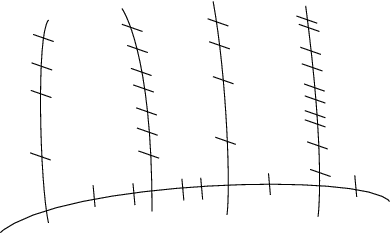
The class associated to the partition in the above expansion has support on , which explains why we call it an inclusion-exclusion principle. This intersection is a moduli space of comb curves as in the figure on page 1.
6.2. Non-equivariant recursions for
Let act non-trivially on so that it leaves the volume form of invariant. Up to isomorphism of , we may assume that the generator is acting with age 1; then the weights of the one-dimensional representations satisfy . The age of the action of a non-trivial group element is given by . In this section we will develop recursions for invariants of the form
| (6.2.1) |
where are group elements of age 1, and is arbitrary, and also the only element for which we allow insertion of a -class. (This implies that for all .)
We want to determine the integral of a summand on the right-hand-side of equation (6.1.2) related to a partition of , after inserting an additional -class at the -th marked point. Let be the elements of .
This term is supported on the intersection , isomorphic to ; so in order to determine the integral of , we will write it as a product of with factors that are pulled back from one of the components above.
The numerator of is the only factor that has terms coming from , while its denominator involves , which is the -class of the node corresponding to the marking on . To examine the numerator more closely, we first factor out :
The largest power of which appears in the last expression is
As the dimension of is , the expression only has a term in the top degree if , which means that acts with age on and acts nontrivially in each coordinate direction. By the balancing condition, is prescribing the monodromy of the node as seen from the component corresponding to . As the integral of is one, the integral of the above product on is if the condition on is satisfied, and 0 otherwise.
On , we are left with the following product:
Here we used the same conventions as for formula (5.2.1), applied to the set (so for example is identified with , which is the -class of a single marking; the term related to in the above product is the denominator of ); and we extended in the obvious way from subsets of to subsets of the quotient set . Now by the remarks in section 5.2, based on lemma A.1.1, this product computes the Chern class of the obstruction bundle on . Its integral is thus given by the equivariant Gromov-Witten invariant
This proves the following recursion:
Proposition 6.2.1.
For an equivariant Gromov-Witten invariant of as in equation (6.2.1) with the assumptions above, let be the set of non-trivial partitions of such that for every , the group element acts with age 1 on , and non-trivial in every coordinate direction. Then the following recursive formula holds:
Here the invariant with superscript “weighted” means the invariant as computed by using the moduli space of weighted stable maps instead of the ordinary moduli space, with weight data chosen as in section 3.4. These invariants are given, up to a multiplication with a monomial in the , by the -th elementary symmetric function of the variables for .
6.3. Recursions for
The recursion of proposition 6.2.1 simplifies further in the case for the diagonal representation of . The only group element of age 1 is . We have for all and . The set contains the partitions of so that every has size for some . The summand for in the formula of proposition 6.2.1 depends only on the sizes of the subsets, not on the actual subsets; if we set , we can thus reduce the above sum to a sum over partitions of , for all with . For any such partition, let be the multinomial coefficient
counting the ways to distribute markings on the different components.
Proposition 6.3.1.
The superscript “weighted” means the same as before; if and , this weighted Gromov-Witten invariant is just given as ; otherwise it is an elementary symmetric function.
A maple program implementing some of these recursions is available from the authors upon request. The numbers match the calculations of [ABK08], [CCIT07a] and [CC07].
As the recursions are linear, it is not hard to invert the matrix and obtain a direct formula. Let . Proposition 6.3.1 implies that
where and for , is the sum over partitions of , with , of the quantity
Let . By inverting the matrix we obtain the formula:
where and it is assumed that . For , the summand is taken to be .
6.4. Inversion of the “mirror map”
The recursion in this case can also be derived from the results in [CCIT07a]. We explained above in section 3.5 that their -function is almost identical (up to high powers of ) to the “weighted -function” .
From general principles of Givental’s formalism they deduce that for the coordinate change , called the “mirror map”, given by
the twisted -function and the twisted -function can be related after setting the dual coordinate of equal to zero:
Our recursive formula can be recovered by comparing coefficients of these two power series; in other words, the sum over partitions in proposition 6.3.1 is a combinatorial inversion of the mirror map .
More precisely, given any two power series , related by
we can recursively recover the coefficients of by comparing coefficients of powers of . If we write and with , the recursion will look exactly as proposition 6.3.1 with the “weighted invariants“ replaced by and the actual invariants replaced by . In particular, setting to the identity power series yields an inversion of the mirror map that can also be a interpreted as a sum over comb curves.
6.5. Equivariant recursions
The methods of this section are sufficient to produce a linear recursion for the equivariant descendant Gromov-Witten invariants of . However, this requires one to allow -classes at every marked point. As in section 6.2, one can use lemma 6.1.1 to expand the equivariant Euler class of the obstruction bundle, and to each partition of one should associate a comb as before, where the -th marked point is on the head of the comb. For each tooth of the comb, we can write the numerator of as
just as in section 6.2. The exponent of which leads to a nonzero integral is determined by the descendant exponents chosen for the marked points in . The integral over the tooth can then be computed using the well-known formula
We are left with a polynomial in , the -class of the node on the main component (and hence our method does not yield a recursion for non-descendant invariants only).
In summary, for each partition of , one gets a linear combination of equivariant Gromov-Witten invariants with fewer marked points, each with a combinatorial factor. These must be summed together and added to the weighted invariant, just as in section 6.2.
Appendix A Combinatorics of divisors on
A.1. Notations for divisors
This section reviews notations for divisors on , some of which is introduced in this paper. The standard relations are reviewed, and a combinatorial proof of a key simplifying relation, used in section 6, is worked out.
First recall the vital divisor , introduced by Keel [Kee92], where is any subset of having at least and at most elements. This divisor is the locus of curves having a node which separates the markings into and . Here complements are always taken within . To make this into a correspondence, assume throughout this appendix that and are subsets of . It is natural to define to be , which comes from the work of de Concini and Procesi [DCP95]. From their point of view, is the pullback of minus the hyperplane class under a sequence of blowups producing from . This sequence of blowups is the same one discussed in section 3.2 in the context of weighted stable maps. Under this blowup description of , is the exceptional divisor of the blowup in the proper transform of the linear space generated by the points labeled by .
The ring is generated by the divisors for , , with relations given by
| (A.1.1) | ||||
| (A.1.2) |
Geometrically, the first relation is due to the fact that the exceptional divisors and are disjoint, and the second is due to the fact that the preimage of the hyperplane in generated by all points except and consists of the proper transform together with all the exceptional divisors for . Fix and choose and . Then relations (A.1.1,A.1.2) imply that
| (A.1.3) |
For any nonempty subset , we introduce the notation
| (A.1.4) |
If , then this recovers the -class at the -th marked point. Indeed, we have for any distinct different from (recalling the convention ),
the last equality following from an inclusion-exclusion argument. By definition, , and we also set for . Finally, we define
for , which we found useful in section 6.
The Chern class formula of theorem 5.1.1 can now be expressed as
| (A.1.5) |
where and are chosen so that . The following lemma shows that if every , this expression is periodic in each with period ; so it defines a continuous, piecewise-analytic function from an -dimensional real torus into the cohomology of with real coefficients. This is used in section 6 to produce recursions for the Gromov-Witten invariants.
Lemma A.1.1.
Let be real numbers, and for any subset , define . Then
| (A.1.6) |
Proof.
For , let
and let
Then it must be shown that . As , it follows that . Moreover, , so . It remains to show that for .
Note that for any divisors ,
| (A.1.7) |
Fix with and , and let be any expression of the form , where is a collection of subsets with and . Then by the following argument. For any , and , so . Moreover,
Since annihilates the first term on the right hand side by (A.1.3) and annihilates the second by (A.1.1), it follows that , completing the verification of the claim.
It follows that one can iterate through all sets with to eliminate those factors from the expression for and apply relation (A.1.7) at each step. Since
it follows that , completing the proof. ∎
If in (A.1.5), one were to add to (and thus add one to each for ) then one would be multiplying by the left hand side of (A.1.6). Therefore does not change after the translation . Using the notational conventions of section 1.5, the formula for makes sense for negative values of , and the same argument shows that it remains invariant under integer translations. It seems natural to regard as coordinates on satisfying .
A.2. Restricting to
It is a standard fact for any proper subset containing at least two elements, , with the node counting as an extra marked point on each factor. The restrictions of divisors and to are easily computed if one uses subsets of for the divisors on the first factor on subsets of the quotient set for divisors on the second factor. So on the first factor, the node counts as the extra marked point that all sets must avoid. For sets , we use and to notate divisors on and we likewise use and for divisors on . Now the following formulas hold for any nonempty set .
| (A.2.1) | |||
| (A.2.2) |
Note that the fourth line of (A.2.1) is another way of writing the standard fact that the restriction of to is the sum of the -classes at the node on the two components. Moreover, the third line of (A.2.2) shows that restricts to as the class of the node on the component corresponding to . So our definition of as ensures that restricts to the class of the node on the other component.
References
- [ABK08] Mina Aganagic, Vincent Bouchard, and Albrecht Klemm. Topological strings and (almost) modular forms. Comm. Math. Phys., 277(3):771–819, 2008, arXiv:hep-th/0607100.
- [Abr05] Dan Abramovich. Lectures on Gromov-Witten invariants of orbifolds, 2005, arXiv:math.AG/0512372.
- [ACV03] Dan Abramovich, Alessio Corti, and Angelo Vistoli. Twisted bundles and admissible covers. Comm. Algebra, 31(8):3547–3618, 2003, arXiv:math.AG/0106211. Special issue in honor of Steven L. Kleiman.
- [AG08] Valery Alexeev and G. Michael Guy. Moduli of weighted stable maps and their gravitational descendants. J. Inst. Math. Jussieu, 7(3):425–456, 2008, arXiv:math.AG/0607683.
- [AV02] Dan Abramovich and Angelo Vistoli. Compactifying the space of stable maps. J. Amer. Math. Soc., 15(1):27–75 (electronic), 2002, arXiv:math.AG/9908167.
- [BG06] Jim Bryan and Tom Graber. The Crepant Resolution Conjecture, 2006, arXiv:math.AG/0610129.
- [BGP08] Jim Bryan, Tom Graber, and Rahul Pandharipande. The orbifold quantum cohomology of and Hurwitz-Hodge integrals. J. Algebraic Geom., 17(1):1–28, 2008, arXiv:math.AG/0510335.
- [BM06] Arend Bayer and Yuri I. Manin. Stability Conditions, Wall-crossing and weighted Gromov-Witten Invariants, 2006, arXiv:math.AG/0607580. To appear in Moscow Math Journal.
- [Cad07] Charles Cadman. Using stacks to impose tangency conditions on curves. Amer. J. Math., 129(2):405–427, 2007.
- [CC07] Charles Cadman and Renzo Cavalieri. Gerby localization, Hodge integrals, and the GW theory of , 2007, arXiv:0705.2158.
- [CC08] Charles Cadman and Linda Chen. Enumeration of rational plane curves tangent to a smooth cubic. Adv. Math., 219(1):316–343, 2008, arXiv:math.AG/0701406.
- [CCIT06] Tom Coates, Alessio Corti, Hiroshi Iritani, and Hsian-Hua Tseng. Wall-Crossings in Toric Gromov-Witten Theory I: Crepant Examples, 2006, arXiv:math.AG/0611550.
- [CCIT07a] Tom Coates, Alessio Corti, Hiroshi Iritani, and Hsian-Hua Tseng. Computing Genus-Zero Twisted Gromov-Witten Invariants, 2007, arXiv:math.AG/0702234.
- [CCIT07b] Tom Coates, Alessio Corti, Hiroshi Iritani, and Hsian-Hua Tseng. The crepant resolution conjecture for type A surface singularities, 2007, arXiv:0704.2034.
- [CG07] Tom Coates and Alexander Givental. Quantum Riemann-Roch, Lefschetz and Serre. Ann. of Math. (2), 165(1):15–53, 2007, arXiv:math.AG/0110142.
- [DCP95] C. De Concini and C. Procesi. Hyperplane arrangements and holonomy equations. Selecta Math. (N.S.), 1(3):495–535, 1995.
- [FP00] C. Faber and R. Pandharipande. Logarithmic series and Hodge integrals in the tautological ring. Michigan Math. J., 48:215–252, 2000, arXiv:math.AG/0002112. With an appendix by Don Zagier, Dedicated to William Fulton on the occasion of his 60th birthday.
- [Giv01] Alexander B. Givental. Gromov-Witten invariants and quantization of quadratic Hamiltonians. Mosc. Math. J., 1(4):551–568, 645, 2001, arXiv:math.AG/0108100. Dedicated to the memory of I. G. Petrovskii on the occasion of his 100th anniversary.
- [Giv04] Alexander B. Givental. Symplectic geometry of Frobenius structures. In Frobenius manifolds, Aspects Math., E36, pages 91–112. Vieweg, Wiesbaden, 2004, arXiv:math.AG/0305409.
- [Has03] Brendan Hassett. Moduli spaces of weighted pointed stable curves. Adv. Math., 173(2):316–352, 2003, arXiv:math.AG/0205009.
- [JK02] Tyler J. Jarvis and Takashi Kimura. Orbifold quantum cohomology of the classifying space of a finite group. In Orbifolds in mathematics and physics (Madison, WI, 2001), volume 310 of Contemp. Math., pages 123–134. Amer. Math. Soc., Providence, RI, 2002, arXiv:math.AG/0112037.
- [Kee92] Sean Keel. Intersection theory of moduli space of stable -pointed curves of genus zero. Trans. Amer. Math. Soc., 330(2):545–574, 1992.
- [LMB00] Gérard Laumon and Laurent Moret-Bailly. Champs algébriques, volume 39 of Ergebnisse der Mathematik und ihrer Grenzgebiete. 3. Folge. A Series of Modern Surveys in Mathematics [Results in Mathematics and Related Areas. 3rd Series. A Series of Modern Surveys in Mathematics]. Springer-Verlag, Berlin, 2000.
- [MM08] Anca M. Mustaţǎ and Andrei Mustaţǎ. The Chow ring of . J. Reine Angew. Math., 615:93–119, 2008, arXiv:math.AG/0507464.
- [Rua02] Yongbin Ruan. Stringy geometry and topology of orbifolds. In Symposium in Honor of C. H. Clemens (Salt Lake City, UT, 2000), volume 312 of Contemp. Math., pages 187–233. Amer. Math. Soc., Providence, RI, 2002.
- [Rua06] Yongbin Ruan. The cohomology ring of crepant resolutions of orbifolds. In Gromov-Witten theory of spin curves and orbifolds, volume 403 of Contemp. Math., pages 117–126. Amer. Math. Soc., Providence, RI, 2006, arXiv:math.AG/0108195.
- [SGA71] Théorie des intersections et théorème de Riemann-Roch. Springer-Verlag, Berlin, 1971. Séminaire de Géométrie Algébrique du Bois-Marie 1966–1967 (SGA 6), Dirigé par P. Berthelot, A. Grothendieck et L. Illusie. Avec la collaboration de D. Ferrand, J. P. Jouanolou, O. Jussila, S. Kleiman, M. Raynaud et J. P. Serre, Lecture Notes in Mathematics, Vol. 225.
- [Tse05] Hsian-Hua Tseng. Orbifold Quantum Riemann-Roch, Lefschetz and Serre, 2005, arXiv:math.AG/0506111.