Mean Field Models of Message Throughput in Dynamic Peer-to-Peer SystemsThis work was in part funded by the Australian Research Council, ARC Discovery Project, DP0451936.
Abstract
The churn rate of a peer-to-peer system places direct limitations on the rate at which messages can be effectively communicated to a group of peers. These limitations are independent of the topology and message transmission latency. In this paper we consider a peer-to-peer network, based on the Engset model, where peers arrive and depart independently at random. We show how the arrival and departure rates directly limit the capacity for message streams to be broadcast to all other peers, by deriving mean field models that accurately describe the system behavior. Our models cover the unit and more general buffer cases, i.e. where a peer can buffer at most messages at any one time, and we give results for both single and multi-source message streams. We define coverage rate as peer-messages per unit time, i.e. the rate at which a number of peers receive messages, and show that the coverage rate is limited by the churn rate and buffer size. Our theory introduces an Instantaneous Message Exchange (IME) model and provides a template for further analysis of more complicated systems. Using the IME model, and assuming random processes, we have obtained very accurate equations of the system dynamics in a variety of interesting cases, that allow us to tune a peer-to-peer system. It remains to be seen if we can maintain this accuracy for general processes and when applying a non-instantaneous model.
1 Introduction
Fundamentally, in a peer-to-peer (P2P) network, messages can only be exchanged between peers that are online state. If a peer is not online then it is offline and no messages are exchanged with a peer while it is offline. When a peer is online then it is available to send and receive messages from other peers. By considering each peer to be in one of these two states and by examining the frequency of state changes over all peers, we describe the churn of the P2P network. A high churn means a high frequency of state changes and vice versa. We can bound the total number of peers, in which case a given peer will continue to alternate between states over time, or we can allow the number of peers to be infinite and consider a finite number of online peers, in which case a given peer may never return to the online state after becoming offline. We call these cases the finite and infinite population models respectively. In both cases there is an expected number of peers that are online, at any given time, when the P2P network is in equilibrium. In this work we focus on P2P networks with a bounded number of peers because we are interested in how the churn affects the message dissemination capacity of the network; though we make some remarks about the infinite population model for interest.
Messages may be generated by users, application processes, data sources or as the result of control traffic, e.g. stabilization or response to changing network conditions, between peers. Using the finite population model we can assume in this work that messages are to be disseminated to all other peers, including to those that may happen to be offline at the time the message was generated. In these circumstances we naturally ask for the time taken for a message to be received by all (or a fraction) of the other peers with the understanding that, as peers change between the offline and online states, all peers may or may not eventually receive the message in question.
As one example, consider a query message that originates at a peer in an unstructured P2P network; where each peer in the network may have some data that is relevant to the query. In a basic network the query message is flooded by each peer evaluating the query, forwarding the message to other peers and possibly responding to the query. Typically each peer that receives the query will delete it after consideration. In the finite population model we ask for the fraction of total peers that received the query message, what we call the query message coverage. In the infinite population model we would ask for the absolute number of peers that received the message. Intuitively, the peers that receive the query message are those peers that were online while the query message was being flooded. We can refine our intuition by considering those peers that changed state, either from offline to online or vice versa, during the time that the query message was being flooded.
In general, messages may be buffered rather than being deleted immediately after processing. If a message is buffered indefinitely by at least one peer then (for a bounded number of peers) the message will eventually be received by all peers, i.e. the coverage will be 100%; this is the case for infinite sized buffers. For a large volume of messages, e.g. consider when all peers in the network are frequently generating queries, and there are limited resources available at the peers, e.g. mobile devices versus desktops, it becomes more practical to place a limit on the buffer size. In this case a message is buffered only for some time and some peers may not receive the message at all. In this work we examine how the size of the buffer relates to the coverage. To do so we also consider the message rate.
1.1 Instantaneous message exchange
To clearly examine the affect from churn and finite buffer size we first eliminate any affects from the sub-communication system (i.e. the Internet in most cases) by allowing any number of message transmissions between online peers to take place instantly; we refer to this as the instantaneous message exchange (IME) model. In this case, e.g., a message that is generated at a peer that is online is instantly communicated to all other peers that are also online at that time of message generation. While this generally is an unrealistic allowance, it allows us to model how churn and finite buffer size places limits on message coverage regardless of the sub-communication system’s ideal performance.
From another perspective The IME model is applicable when churn is sufficiently low relative to the message propagation time through the network; in the sense that the network appears to be static from the perspective of a single message propagation.
Aspects such as bandwidth and latency in the sub-communication system lead only to further limitations; i.e. in this work we are concerned with how churn places a limit on the message coverage and we make ideal or best case assumptions about other aspects, which can otherwise only lead to the message coverage being further limited.
1.2 Related work
To the best of our knowledge there are currently no results that have proposed the IME model as a starting point. The dynamics of the IME model can be analyzed by taking an epidemic information dissemination approach [4], sometimes called randomized rumor spreading [5]. Based on analysis of infectious diseases [1], the two basic models are infect and die and infect forever. In the infect and die model, a disease or message is communicated for only a single round and then the peer no longer participates. In the infect forever model the peer can continue to communicate the message forever. For the very basic case in the IME model, i.e. a single message broadcast, the infect forever model is applicable. However, for a stream of messages that are being broadcast then the situation is a non-trivial combination of infect and die (because of the finite buffer limitation) and infect forever (because peers can continue to communicate a message until they receive a subsequent message). Also, epidemic information dissemination usually assumes that subsequent generations of infected peers are selected at random from the population. In the IME model this is not true because a peer can only receive a message when it is online.
The most closely related work is that of Yao, Leonard et. al. [10]. They model heterogeneous user churn and local resilience of unstructured P2P networks. They also concede early that balancing model complexity and its fidelity is required to make advances in this area. They examine both the Poisson and Pareto distribution for user churn and provide a deep analysis on this front. Their work focuses on how churn affects connectivity in the network and we have separated this aspect from our work and concentrated on message throughput.
Other closely related work concerns mobile and ad hoc networks, and sensor networks, because these applications require robust communication techniques and tend to have limited buffer space at each node. The recent work of Lindemann and Waldhorst [6] considers the use of epidemiology in mobile devices with finite buffers and they follow the seven degrees of separation system [8]. In particular they use models for “power conservation” where each mobile device is ON with probability and OFF with probability . Their analytical model gives very close predictions to their simulation results. In our work we describe these states using arrival rate, , and departure rate, , which allows us to naturally relate this to a rate of message arrivals, . We focus solely on these parameters so that we can show precisely how they affect message coverage rate.
Other closely related work such as in [7] looks at the rate of file transmission in a file sharing system that is based on epidemics. The use of epidemics for large scale communication is also reviewed in [9]. The probabilistic multicast technique in [3] attempts to increase the probability that peers receive messages for which they are interested and to decrease the probability that peers receive messages for which they are not interested. Hence it introduces a notion of membership which is not too different to being online/offline. Autonomous Gossiping presented in [2] provides further examples of using epidemics for selective information dissemination.
1.3 Organization
In Section 2 we describe our IME model and show the derivation of equations that accurately predict its behavior. We compare the analytical results with simulations. In Section 2.3.4 we examine the use of the model to choose message rates appropriate for the churn. In Section 3.1 we provide a derivation of the buffer and multi-source cases. We conclude the paper in Section 4 with some overall observations and future work.
Table 1 provides the notation used in this paper. Generally, when a function, , is provided with a subscript or then the function is representing either the offline or online case resp, e.g. and in Table 1. Later in the paper we extend this subscript notation to represent more complicated cases. For stochastic processes like we use as the expected value and we use as the normalized expected value.
| number of peers | |
| arrival rate of a peer | |
| departure rate of a peer | |
| mean number of peers offline | |
| mean number of peers online | |
| time | |
| coverage of a single message at time | |
| rate of message arrivals | |
| average coverage of a message in a message stream | |
| average base coverage a message in a message stream | |
| (extended) coverage rate | |
| fraction of messages of type (e.g. type , , , etc.) | |
| size of the buffer | |
| number of source peers |
2 IME model and analytical formulation
We begin this section with a basic description of the IME model using queueing theory. We then provide a basic analysis for a single message broadcast. Results from the basic analysis are used throughout the paper. Simulation results are compared to for each of the results.
2.1 Instantaneous message exchange model
Consider a set of peers where each peer, has a state, where 0 means offline and 1 means online. We say that a peer is online or offline to mean which state it has. Let each peer change from offline to online at a random time according to an “arrival” rate, , such that:
where is the mean time taken to change state from offline to online, with a cumulative distribution function given by the Poisson distribution11 1 In future work we shall investigate variations of the Pareto distribution for peer lifetimes.. Similarly is defined as the mean time to change state from online to offline with “departure” rate, . In other words, each peer spends a proportion, , of its total time arriving and departing respectively; shown in Figure 1. The peers are described by an queueing system (where ) as shown in Figure 2.

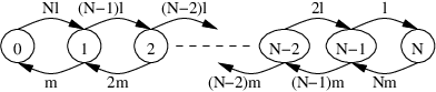
Using Figure 2, if we let be the number of online peers, then we can write:
Hence the system reaches an equilibrium when the number of online peers is
and equivalently when the number of offline peers is
In this work we assume that the system is in equilibrium and we use and as continuous variables.
2.2 Single message broadcast
Consider the case when a peer, called the source, is chosen uniformly at random from and at time that peer generates a new message. The notion that messages can be transmitted instantly between online peers is described by the rule: peer has received the message by time iff there is some such that peer was online with some other online peer that already had the message, at time . A peer that remains offline up to (but not including) time , cannot have received the message before time .
Let be a continuous time, discrete space, stochastic process that counts the number of peers with the message by time . We say that is the coverage of the message at time . At time the source peer is initially offline with probability and online otherwise. Hence we consider which is the weighted average of two different coverage functions, and for the initially offline and initially online cases respectively.
For generality, we allow messages to be generated even if/while the peer is offline. This is generally required in the case that, e.g., the peer is generating or collecting data which is independent of whether the peer is online or not. The special case when messages are not generated at a peer that is offline, is then a simplification of the general case.
2.2.1 Source peer starts online
In this case, coverage starts at time . After time (for some integer ) the average number of peers that have the message is
| (1) |
In this work we mean field analysis in terms of , since a P2P network is expected to consist of a large number of nodes. The technique simplifies the derivations in some cases; equations in terms of are however always possible and we use both forms throughout.
2.2.2 Source peer starts offline
If the source peer starts offline then it becomes online with probability at time , i.e. at an average time of . Hence is the convolution with :
| (2) |
The constant and last term of the integration represent the diminishing constant which accounts for the “fraction of the source peer” that has not yet become online. Before the source peer becomes online, or more specifically at time , . As increases, the probability increases that the source peer becomes online and so too does the average coverage increase, where the first term accounts for the fraction of the source peer that has become online.
2.2.3 Expected coverage
Of course, the observed coverage either starts from time or starts at an average time of . The expected coverage in Eq. 3 represents the average of these two cases. Figure 3 shows 10 simulation runs when and . The simulation tool is described in the Appendix for reference. The points in a series indicate times when a new peer received the message. The solid lines are and (the functions are plotted starting from time 0.1). Note that is only an average, and is not representative of either the online or offline cases.

2.2.4 Basic simulation results
2.3 Multiple message broadcast - unit message buffer
Let messages be generated at a source peer with rate and consider a sequence of generation times . Apply the rule that each peer discards a current message in favor of a newer message and does not receive messages that are older than the current message. A message is said to be skipped by a peer if that message is not received by the peer because a newer message has already been received. Figure 4 shows an example realization in time of events that occur at the source peer. It also shows a number of numerical quantities that are important for the equations. A solid vertical line represents the source peer moving from offline to online. A dashed vertical line represents moving from online to offline. Arrival of a new message is shown by a and the message numbers are given at the bottom of the figure for reference.

We are interested in computing the average coverage of a message in a message stream such as that shown in Figure 4. Since messages are discarded in favor of new ones, the coverage of any given message is limited. If is the coverage of message in the message stream of messages then we define
as the average coverage of a message in a message stream.
In Figure 4 note that message arrives while the source peer is online, therefore it is immediately received by all other peers that are online and the coverage of that message at time (its arrival time) is immediately . Shortly after time , the source peer goes offline. Message 1 continues to be transmitted between new peers that enter the network and its coverage increases. The arrival of messages 2, 3 and 4 does not hinder the transmission of message 1 because the source peer is still offline. The coverage of these messages is exactly 1. However, shortly after the arrival of message 4, the source peer goes online. At this point, all online peers receive message 4 and the coverage of message 4 jumps to . The coverage of message 4 continues to grow until the arrival of message 5, which is immediately transmitted to all online peers (overwriting message 4 due to the unit buffer restriction). Message 5’s coverage increases until the arrival of message 6, and so on.
Note that messages 1, 6 and 8 are the last messages to arrive in each interval for which the source peer is online. These messages continue to increase their coverage until the source peer moves back online and has a newly arrived message in the mean time. E.g., if message 7 did not arrive then message 6 would have continued to grow until message 8 arrived. Also note that messages 2, 3 and 9 were not received by any other peers and never will be, their coverage remains at 1.
We identify four categories of messages (the naming scheme simplifies our notation later), listed in Table 2.
| A message that is the last one to arrive before the peer moves from online to offline (e.g. messages 1, 6 and 8). | |
| Messages that arrive while the peer is online but not a message (e.g. message 5). | |
| A message that is the last one to arrive before the peer moves from offline to online (e.g. messages 4, 7 and 10). | |
| Messages that arrive while the peer is offline but not a message (e.g. messages 2, 3 and 9). |
When only one message arrives in an interval (by interval we mean either the online or offline time interval) then that message is a or (i.e., in this case there are no or messages in that interval).
Intuitively,
because at low message arrival rates each message has ample time to cover all peers. Of course, when then the message throughput is low which is undesirable.
As a consequence of our IME model, note that any message that achieves a coverage of greater than 1 will achieve a coverage of at least . We call this the base coverage and we note that the average base coverage is the average coverage of a message as the message rate becomes large:
All messages reach exactly peers (immediately on their arrival), all messages reach only 1 peer (the source peer) and the number of and messages becomes negligible.
Since in the IME model, does not approach 0 as , the natural coverage rate (or message-peer throughput) is unbounded. However, we observe that in this case the average coverage approaches the constant and so while the rate of messages is arbitrarily large, the messages are received by only a fixed fraction of the peers.
For these reasons we are interested in coverage achieved beyond the base coverage and we formulate what we call the mean extended coverage rate:
| (4) |
In this paper we simply refer to Eq. 4 simply as the coverage rate which has units message-peers per time unit. When is small, while a single message will cover all of the peers, there are not many messages and the overall number of messages received by the peers is small; ultimately the coverage rate falls to zero. When is large, while a number of peers , at any one time, may receive a large number of messages the actual coverage of a single message is at most and the extended coverage drops to 0.
To analyze Eq. 4, we derive an equation for by combining individual equations for the different message categories.
2.3.1 Fraction of appearance for each message category
Clearly, of all messages will arrive while the source peer is offline, i.e. they are and messages, and similarly for and messages. We need to know the fraction for each category; in Figure 4 we use to represent the fraction of messages that are and to represent the fraction of messages that are . Then the fraction that are is:
| (5) |
and similarly for the fraction:
| (6) |
For a given message rate , in the time interval we have messages arriving on average. The fraction is derived by summing the individual probabilities of messages arriving before the state change from offline to online occurs, where we are weighting the event that messages become messages. This is divided by the average number of messages that arrive because we are interested in the fraction of such messages, not the total. The equation becomes:
| (7) |
Similarly:
| (8) |
2.3.2 Coverage of each message category
The average coverage of messages, , is trivially 1 since these messages do not have a chance to be communicated to other peers. The average coverage of messages, , follows the single message coverage function from Eq. 1, , where the average time is . Since is non-linear we integrate the growth over all possible times:
The coverage of and messages is more difficult to model because their average coverage time is affected by whether the peer is online or offline when the subsequent message arrives. If the peer is offline then the time increases by an amount given by the average time for the peer to become online again. We therefore further categorize these messages as , , and messages, depending on whether the peer is online or offline when the subsequent message arrives.
For messages we integrate over the shaded regions shown in Figure 5 and we essentially round up to the interval. For messages we integrate exactly to the time . The integration is similar for and messages, except that the integration time begins at the beginning of a interval rather than at the beginning of a interval.

Let , then the integrations become:
We show here only the expressions when . For messages:
| (11) |
Similarly for messages:
| (12) |
2.3.3 Total coverage equation
Each of the coverage functions contribute according to the fractions in Eqs. 8, 7, 10 and 9. Hence:
| (13) |
Note that for the fractional term becomes 0 and all other terms are interchangeable.
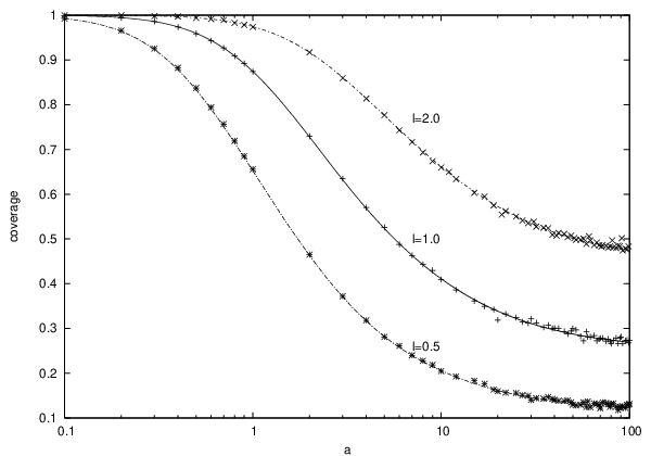
While inspection of the final coverage equation does offer some insight, we omit it due to its complex structure. Figure 6 shows the results from simulations. Each point is the average of 10 trials with , , 1000 messages transmitted and other parameters as shown. The coverage is normalized. Clearly, as increases then the coverage decreases. Note that as , the coverage limits to . The precision of the simulation results decreases as increases because the simulation is run for a fixed number of messages and hence an increased leads to a decreased run time. The solid lines represent the coverage as evaluated from Eq. 13.

Clearly, if a specific coverage is required (at least) by an application then takes a limited range. E.g., if the application requires a coverage of at least 0.6 of the total peers, in a case where then from Figure 6, is limited to be less than roughly 1.


2.3.4 Coverage rate
We plot the coverage rate from Eq. 4 in Figure 7(a). When is low, the coverage rate is close to . The coverage rate is never equal to and Figure 7(a) shows as a reference. As increases (or equivalently as decreases) then it is possible to achieve a higher coverage rate because peers spend more of their time in the network.
The coverage rate saturates with large and we have:
| (14) |
These limits are shown in Figures 7(a) and 7(b) as horizontal dashed lines.
Note that:
which is a consequence of there being no message transmission rate limits on individual peers.
Figure 7(b) shows that the coverage rate exhibits a local maximum which approaches Eq. 14. Hence, for parameters in these ranges it is possible to achieve a close to maximum coverage rate at a relatively small . For example, when and then from Figure 7(b) we have to achieve a coverage rate that is very close to the maximum, which would not otherwise be met until .
Simulation results (not reported here) show that these coverage rates are highly susceptible to deviations from the average coverage. Therefore, this analysis can serve as a rough guide, in the sense that while a value of may be computed as giving a particular coverage rate, an observed coverage rate (which is necessarily over a finite range) is likely to deviate from the theoretical prediction.
3 Message buffer and multiple sources
In this section we formulate the coverage for the cases when peers can buffer messages and when there are multiple sources of messages.
3.1 Using a -buffer
We calculate coverage for the -buffer case similarly to the unit buffer case, dividing messages into separate categories. In this section we redefine the and fractions to be with respect to the -buffer case. We also define further fractions.
3.1.1 Message categories and their fractions
As in the unit buffer case we consider the fraction of messages that arrived in the period when the source peer was either online or offline and was pushed from the buffer before the peer changed its state; which we call and , meaning fraction of and messages respectively, where buffer size is equal to . In this case we calculate the fraction by summing the individual probabilities of messages arriving before the state changes from offline to online, where we are weighting the event that messages become messages. As in the unit buffer case, this is divided by the average number of messages that arrive. So, the equations become:
| (15) |
Similarly:
| (16) |
Unlike the unit buffer case we now have to consider a number of both and messages. We say that a message is an or message to mean that messages arrived before the peer changes the state.
Each and message will have it’s own rate and coverage because each of them will have a different coverage time. This is because there is, e.g., an average time of between message and message , and so on.

An example for is shown in Figure 8. In the figure:
-
: Message 1 is propagated until messages 3 comes, similarly message 2 propagates until message 4 is generated. In other words both of messages 1 and 2 get coverage until 2 more messages arrive.
-
: Message 3 is propagated until the peer goes offline, and then it continues to propagate until at least one more message has arrived after message 4 and the peer has come back online.
-
: Message 4 is propagated until at least two more messages are generated, similarly to the previous example.

We derive , , as shown on Figure 9:
Similarly:
3.1.2 Coverage of messages
All messages propagate until at least subsequent messages have been generated. So we look at the probability of the -th message arriving at time . We use the Erlang distribution to compute the probability of the -th message arriving:
| (17) |
3.1.3 Coverage of messages
As in the unit buffer case we consider and messages. A message is propagated while it exists in the buffer; to be pushed out of the buffer, more messages have to arrive into the buffer. Because we are considering only time periods after the period in which message was generated, we know that messages have already arrived. Thus only more messages have to arrive to push the message from the buffer. We are interested in the probability of the -th message arriving in a subsequent online period. The propagation starts from the point when the -th message was generated, i.e we are interested in the coverage after time . We use the Erlang distribution again:
| (18) |
Similarly for , we modify the result for to get:
| (19) |
3.1.4 Coverage of messages
We use equations derived for unit buffer case, except as for messages we wait until the -th message arrives:
| (20) |
| (21) |
Note that the time within has no offset because it does not matter how recent a message arrived before the peer became online, propagation starts only after the peer becomes online.
3.1.5 Total coverage equation for -buffer case
We add the coverage of each message type to get total coverage:
| (22) |
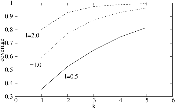
Figure 10 shows theoretical results for values 1,2,3 and 5 with fixed . Figure 11 shows a comparison of simulation runs with , and 1000 messages in the network. Figure 12 shows the theoretical increase in coverage as increases, for various . E.g., to achieve a coverage of at least 0.7 when we need to have a buffer size of at least 4. Clearly, increasing increases the coverage. Furthermore, since the fraction of and messages becomes insignificant.

3.2 Multiple source model
In this section we consider the case when multiple peers are generating messages. We maintain the message arrival rate on a network wide basis, i.e. if there are sources in the network each peer generates messages with rate rate.
We make the following simplifications:
- •
We ignore messages that occur on the peer when the peer is offline. These kinds of messages were included in the previous sections and could be removed if desired. This simplification limits our model in this section to applications where messages are only generated on peers that are currently online.
- •
We assume that is sufficiently large. Small values for , experimentally determined to be less than about 10, lead to a large variety of message classes that we have not yet simplified. Practical values of are easily sufficient to justify this simplification.
The simplifications allow the multiple source case to be a direct result of the single source case.
In our model, arriving messages are randomly assigned to one of the peers and so if is sufficiently large then a new message arriving at a peer has a probability of of arriving on a online peer (these are the messages) and it arrives on an offline peer otherwise (these are the messages). Our analysis however takes into account that some source peers may not be online at some times, by allowing the possibility of messages but then ignoring them for coverage rate equations. The messages also never enter the buffer and so they do not reduce the coverage that way either.
Under the aforementioned circumstances, we consider messages in different classes determined by the number of subsequent messages that occur before the next message, to make messages in total. Clearly the probability for each class is a Bernoulli trial, and the time for messages to occur is given by the Erlang distribution similarly to Eq. 17. We arrive at a coverage for the unit buffer size:
Note that the coverage of a message in the multisource case is the same for all of the sources. If we are considering a buffer of size then we need to consider the arrival of messages that are inter-dispersed among the messages and we see that there are combinations. Therefore we obtain:
Figure 13 shows the coverage over a large range of for nodes and . Different values of are shown. The coverages in this section cannot in general be compared with the coverages of the previous section because the previous section included messages that reduced the coverage. Note that the theoretical coverage can be seen, especially for , to be slightly lower than the simulation. This is due to the assumption that is sufficiently large. The assumption becomes worse as becomes smaller because the effective number of source peers that are online reduces.

The increase in coverage versus is shown in Figure 14. Numerical computation of the theoretical values became inaccurate beyond . Note that the chart is for the case when . Also, again the theory slightly undershoots the simulation result as becomes smaller.

Be aware that the value for shown in Figures 13 and 14 are “net” or “total” messages rates. Each peer is providing messages at a rate of only . Therefore for and , the effective rate of a message stream from a given peer is only per second. Thus, the coverage rate for that peer is similarly less, even though the coverage of the messages is the same. In other words, considering Figure 13, if we look at the coverage at we should consider the rate of messages from a single peer to be only and the coverage rate is then 100 times worse than the single source case. Increasing buffer size can allow us to increase without sacrificing coverage and hence to maintain a steady effective message rate per peer.
Figure 15 shows the theoretical smallest value of that maintains a given coverage as increases. Clearly the buffer requirements increase proportionally to the message rate.

4 Conclusion
We have proposed the Instantaneous Message Exchange (IME) model as a fundamental approach for analyzing the affect of churn on streaming message rates. We derived very accurate equations to describe the behavior of the P2P system and we showed how the equations can be used in various ways to determine good system settings. E.g., we can choose appropriate limitations on message transmission rates with respect to churn (or vice versa) in order to achieve high message throughput. We can also see how buffer size enhances the message throughput and how the number of source peers affects these relationships.
In our analysis we have attempted to provide the most accurate descriptions of the system, over all ranges of parameters. In a number of cases the equations are complicated, including three or four complicated terms that are significant at different ranges of the parameters. The IME model was instrumental in allowing us to derive these equations. It remains to be seen whether we can maintain the accuracy of the theoretical work while moving towards a non-instantaneous model.
Future work includes: (i) including peer bandwidth and network delay limitations, (ii) examining more general communication patterns, (iii) using a Pareto distribution or other more suitable distribution from trace data and (iv) developing algorithms that reach the maximum coverage rates.
[Simulation tool]
We developed a basic simulation tool to test our models against. In a nutshell, the simulator is event based and maintains states for peers, including whether each one is online or offline, which messages it has received or sent, etc. The events of the simulator include message generation events (i.e. a peer generates a message), and transition events from online to offline and vice versa. Events for the transmission of a message from one peer to another are not part of the IME model and are therefore not required in the simulation. Message transmission is purely a consequence of message generation and peer online/offline states and transitions between these states.
The simulation begins by assigning each peer as online or offline, with probability and resp. In the single message case the simulation then chooses a peer at random and runs until the message has been received by all peers. For the message stream case the simulation continues to run until a given number of messages have been generated. A sufficiently large number of messages need to be generated in order for the observed results to be independent of the starting configuration of online/offline peers, in other words depending on , and . An appropriate number of messages was set experimentally. For the multiple source case the simulation randomly chooses peers as source peers.
Event times are real numbers and the simulator orders all pending events and processes one event at a time. Following is the brief explanation of what happens after each event:
- 1.
Message generation:
- (a)
Peer was online:
- •
Send new message to all of the online peers.
- •
Compute next message generating event for that peer.
- •
- (b)
Peer was offline:
- •
Compute next message generating event for that peer.
- •
- (a)
- 2.
Changing from online to offline:
- •
Schedule the next time to change to online.
- •
- 3.
Changing from offline to online:
- •
Merge buffers with all online peers to produce the buffer with newest messages; see notes below.
- •
Send that buffer to all of the online peers.
- •
Schedule the next time to change to offline.
- •
Notes:
- •
An invariant of the simulation is that at any point in time the buffers of the online peers are identical. This is a consequence of the IME model. If bandwidth or latency for message transmission were taken into account then the invariant would be broken.
- •
Each message is assigned a number such that message is newer than message only if , i.e. message was generated later than message . A buffer is always sorted by the message number. The buffer is changed due to: (i) new message coming into the network; or (ii) a node that has newer messages than some of the messages in the online peers’ buffers, enters the network. In the first case the newer message is appended to the buffer when the current buffer size is less than ; if the current buffer size is equal to then the oldest message of the buffer is pushed out. In the second case the buffers of the just arrived peer and any online peer are merged so that the merged buffer has the newest messages of the union of those two older buffers. Each of the online peers then has the merged buffer.
References
- [1] N. T. J. Bailey. The Mathematical Theory of Infectious Diseases and its Applications. Griffin, 2nd edition, 1975.
- [2] A. Datta, S. Quarteroni, and K. Aberer. Autonomous gossiping: A self-organizing epidemic algorithm for selective information dissemination in wireless mobile ad-hoc networks. Technical Report EPFL Technical Report IC-2004-07, Swiss Federal Institute of Technology, 2004.
- [3] P. T. Eugster and R. Guerraoui. Probabilistic multicast. In Proceedings of the International Conference on Dependable Systems and Networks, pages 313–322, 2002.
- [4] P. T. Eugster, R. Guerraoui, A. M. Kermarrec, and L. Massoulie. Epidemic information dissemination in distributed systems. Computer, 37(5):60–67, 2004.
- [5] R. Karp, C. Schindelhauer, S. Shenker, and B. Vöcking. Randomized rumor spreading. In Proceedings of the 41st Annual Symposium on Foundations of Computer Science - FOCS, pages 565–574. IEEE Computer Society, 2000.
- [6] C. Lindemann and O. P. Waldhorst. Modeling epidemic information dissemination on mobile devices with finite buffers. In SIGMETRICS, pages 121–132, 2005.
- [7] C. X. Mavromoustakis and H. D. Karatza. Segmented file sharing with recursive epidemic placement policy for reliability in mobile peer-to-peer devices. In Proceedings of the 13th IEEE International Symposium on Modeling, Analysis, and Simulation of Computer and Telecommunication Systems (MASCOTS), page 8 pages, 2005.
- [8] M. Papadopouli and H. Schulzrinne. Effects of power conservation, wireless coverage and cooperation on data dissemination among mobile devices. In MobiHoc ’01: Proceedings of the 2nd ACM international symposium on Mobile ad hoc networking and computing, pages 117–127, 2001.
- [9] W. Vogels, R. van Renesse, and K. Birman. The power of epidemics: Robust communication for large-scale distributed systems. ACM SIGCOMM Computer Communications Review, 33(1):131–135, 2003.
- [10] Z. Yao, D. Leonard, X. Wang, and D. Loguinov. Modeling heterogeneous user churn and local resilience of unstructured p2p networks. In Proceedings of the 2006 14th IEEE International Conference on Network Protocols, pages 32–41, 2006.