Non-Metric Gravity II: Spherically Symmetric Solution,
Missing Mass and Redshifts of Quasars
Abstract
We continue the study of the non-metric theory of gravity introduced in hep-th/0611182 and gr-qc/0703002 and obtain its general spherically symmetric vacuum solution. It respects the analog of the Birkhoff theorem, i.e., the vacuum spherically symmetric solution is necessarily static. As in general relativity, the spherically symmetric solution is seen to describe a black hole. The exterior geometry is essentially the same as in the Schwarzschild case, with power-law corrections to the Newtonian potential. The behavior inside the black-hole region is different from the Schwarzschild case in that the usual spacetime singularity gets replaced by a singular surface of a new type, where all basic fields of the theory remain finite but metric ceases to exist. The theory does not admit arbitrarily small black holes: for small objects, the curvature on the would-be horizon is so strong that non-metric modifications prevent the horizon from being formed.
The theory allows for modifications of gravity of very interesting nature. We discuss three physical effects, namely, (i) correction to Newton’s law in the neighborhood of the source, (ii) renormalization of effective gravitational and cosmological constants at large distances from the source, and (iii) additional redshift factor between spatial regions of different curvature. The first two effects can be responsible, respectively, for the observed anomaly in the acceleration of the Pioneer spacecraft and for the alleged missing mass in spiral galaxies and other astrophysical objects. The third effect can be used to propose a non-cosmological explanation of high redshifts of quasars and gamma-ray bursts.
I Introduction
This is the second paper in the series devoted to the detailed study of the non-metric theory of gravity introduced in Krasnov:2006du; Krasnov:2007uu. As in the case of general relativity (GR), one of the first applications of any theory of gravity must be the description of the geometry of a strongly gravitating object — a black hole. This is the basic aim of the present paper, in which we obtain and analyze the spherically symmetric vacuum solution. The considerations of this work will also serve as an illustration to the rather abstract formalism of Krasnov:2007uu.
The theory of gravity under investigation is defined by the action
| (1) | |||
Here, is a (complex) Lie-algebra valued two-form (the indices belong to the Lie algebra), is the curvature of the Lie-algebra valued connection , is a traceless symmetric “Lagrange multiplier” field, and is the Newton’s constant. The function is a function of two scalar invariants that can be constructed from and is responsible for the departure of the theory under consideration from GR. The constant part of the function is (a multiple of) the usual cosmological constant .
The theory with action (1) modifies the Plebański self-dual formulation of general relativity Plebanski:1977, in which . In the Plebański theory, the field , according to the equations of motion, can be canonically decomposed into products of tetrad basis one-forms, which then define a unique distinguished metric satisfying the Einstein equation. With the appearance of a nontrivial function in (1), this property is no longer valid: the arising metric is defined only up to a conformal factor, and it does not, in general, satisfy the vacuum Einstein equations.
The nature of this modification of gravity is quite special and deserves a few words. In the numerous existing schemes of modified gravity, one usually deals with a metric theory and modifies the Hilbert–Einstein action by introducing extra degrees of freedom — either by increasing the number of derivatives (higher-derivative gravity), or by introducing extra fields (scalar-vector-tensor theories), or by considering extra dimensions (braneworlds). Nothing of the listed takes place in our generalization: the theory remains four-dimensional, there are no extra fields, the number of derivatives is not increased, and, as in GR, there are still just two propagating degrees of freedom, as can be seen from the canonical analysis of the theory; see, e.g., Bengtsson:2007zx. This is achieved by first recasting the theory in a form which does not contain any metric Plebanski:1977, and then modifying the theory in this non-metric form. It is thus important to stress that the term “non-metric” is used here not in the sense that some additional degrees of freedom are present along with the usual metric, but in the sense that metric does not even appear in the formulation of the theory.
The difference between our modified gravity and a variety of other approaches can also be seen from the fact that our theory, while modifying the spherically symmetric solution, does not modify the formal general-relativistic cosmological equations. Indeed, due to the high symmetry, the field , which is a close analog of the Weyl curvature spinor in our theory, is identically zero for cosmological solutions, which then coincide with those of general relativity with a cosmological constant determined by . However, any departures from homogeneity and isotropy will be essential, so that the evolution of perturbations in our theory will, in principle, be different from that in the concordance LCDM cosmology. This issue will be studied separately.
A specific choice of the function uniquely fixes a theory from the class (1). One way of fixing the form of this function is to regard it as an effective quantum contribution to the original classical action. In this respect, it was argued in Krasnov:2006du that the class of theories (1) is closed under the renormalization-group flow. The conjecture of asymptotic safety applied to the case at hand then asserts the existence of a non-trivial ultra-violet fixed point of the renormalization-group flow described by a certain function . It would then make sense to choose this fixed-point function in (1) because the quantum field theory so defined would have extremely appealing properties: the action would not get perturbatively renormalized, describing an essentially finite quantum theory of gravity. This gives a possible scenario for fixing from the theoretical side.
In a pure quantum theory of gravity, the Planck scale is the only scale that can enter the renormalized action. However, once the theory is coupled to matter, the corresponding quantum loops in Feynman diagrams will also affect the function . Thus, it should be expected that the ultra-violet fixed-point function will contain more than one physical scale. Qualitative features of the function can be anticipated from the fact that, as we shall see in this paper, a theory with a non-constant function in many respects behaves like a theory with physical parameters depending on the scale. Indeed, as we shall see, the function itself will receive an interpretation of a curvature-dependent cosmological “constant”. Another effect is that passing between spatial regions of different curvature generally introduces a renormalization in the strength of the gravitational interaction. All this is strongly suggestive of the renormalization-group flow phenomena, where one has to identify (having the dimension of the curvature) with the energy scale squared. The crucial difference between our scheme and the renormalization-group flow familiar from the framework of effective field theory is that similar effects arise here in a diffeomorphism-invariant context. This renormalization-group interpretation suggests that the function must look as a sequence of plateaus, with crossover regions between plateaus corresponding to the scales where new physics (new degrees of freedom) come into play. This discussion motivates some assumptions we make about the form of the function in the section where we discuss possible long distance modifications of gravity.
Of special importance is the question of coupling our theory of gravity (1) to other fields. As was discussed in Krasnov:2007uu, coupling to Yang-Mills fields (or electromagnetic field) is seamless, and the action described in CDJ extends to the non-metric situation without any problem. This action tells us how massless particles such as photons interact with gravity and predicts their motion in a non-metric background. It is found that, in the approximation of geometric optics, photons move along null geodesics of the metric determined by the field . The ambiguity in the choice of the conformal factor discussed in detail in Krasnov:2007uu does not affect this conclusion because the paths of null geodesics (but, of course, not the affine parameter along them) are independent of this choice. An important issue that has not yet been addressed in the framework of non-metric gravity and that prevents us from a complete analysis of the physical predictions of theory (1) concerns coupling to (massive) matter degrees of freedom. The action for a massive field of spin proposed in CDJ for the Plebański formulation of general relativity turns out to be incompatible with the non-metric character of the theory under investigation, hence, calls for revision.
Quantitative predictions of our theory, e.g., concerning the motion of stars and gas in galaxies, will depend on the details of the coupling of massive matter to the basic gravitational degrees of freedom. However, its certain general features can already be described in the absence of these details. For instance, in the domains of “metricity,” in which the function is almost constant (where its dimensionless derivatives ), the present theory of gravity behaves very closely to general relativity, and it is quite reasonable to expect that matter will also behave accordingly, moving relativistically in the background of the arising metric. Assuming that several such domains of “metricity” exist at different scales of curvatures, we find that the effective gravitational mass of a central body is different in the corresponding spatial regions. From this simple observation one can conclude that the effective gravitational mass of a body continuously depends on the distance to this body even in the case of general function — the effect of scale-dependence of the gravitational coupling which was mentioned above. One can use this property to account for the phenomenon of missing mass observed in gravitating objects such as spiral and elliptical galaxies. Another interesting general prediction of the present theory is the appearance of an additional redshift factor between regions of different space-time curvature. As we point out in this paper, this effect can be used to account for the observed high redshifts of quasars and gamma-ray bursts. However, practical use of these features of the new theory to explain physical phenomena requires the specific knowledge of the underlying function together with the analysis of the physical content and interpretation of the theory. This will be the subject of the future work.
The organization of the paper is as follows. To obtain a spherically symmetric solution, we first obtain an ansatz for the symmetric field . This is done in Sec. II, in which we also analyze consequences of the modified “metricity” equations. The field equations are obtained in Sec. III. Solutions are analyzed and interpreted in Sec. IV. Possible modifications of gravity are discussed in Sec. V, and possible physical effects in Sec. VI. Our results are summarized in Sec. VII. In the appendix, we give a detailed proof of the static property of the spherically symmetric solution in the theory under consideration and discuss in more generality some details of the large-distance modifications of gravity.
II Spherically symmetric ansatz and metricity equations
II.1 Spherically symmetric Lie-algebra-valued two-form
The most general spherically symmetric Lie-algebra-valued two-form can be obtained from the condition that an rotation corresponds to a gauge transformation. There exists standard technique in the literature allowing one to obtain the relevant expression; see, e.g., Brodbeck:1996ma. One gets:
| (2) |
Here, is the standard set of spherical coordinates, and , , , are functions of and only. The symbols denote the generators , where are the Pauli matrices. As it turns out, it is much more convenient to work not with the adjoint, but with the fundamental representation of . This amounts to working in the spinor formalism. We used spinor formalism rather heavily in Krasnov:2007uu, and will continue to do so in this paper. To pass from the form of the fields to their spinor representation one has to replace every lower-case Latin index by a symmetric pair of unprimed spinor indices. Equivalently, every Lie-algebra-valued field gets replaced by a matrix-valued field. Thus, it will be convenient to rewrite the above ansatz for in terms of the matrices
| (3) |
which are related to as , , . We have:
| (4) |
It is not hard to show, and this fact was used heavily in Krasnov:2007uu, that, by a convenient choice of the spinor basis, the spinor counterpart of the quantity can be put into the form
| (5) |
The functions and are related to the invariant characteristics of :
| (6) |
In view of (6), one can regard as a function of and .
In the spherically symmetric case, the field has the form
| (7) |
where , , are the natural Euclidean coordinates realizing the group of rotations, and . This condition implies in (5), and the field is parameterized by a single function :
| (8) |
In other words, the Lagrange multiplier field must be algebraically special, of type . This is, of course, exactly the property of in a spherically symmetric solution of the usual GR. This property remains unchanged in the non-metric theory of gravity under consideration.
II.2 “Metricity” equations
With the above ansatz for the field, it is easy to compute the quantity that appears in the metricity equations — the equations stemming from (1) as the field is varied. These equations are discussed in Krasnov:2007uu in great length, and we will not repeat that discussion here. We just note that, as it is easy to check, the quantity , with given by (2) above, is diagonal as a matrix. This implies that the matrix , which is the traceless part of in view of the metricity equation, is also diagonal. Hence, must be identically zero in view of equation (26) of Krasnov:2007uu. The property ensures this condition, in particular, if the function is a regular function of its arguments (6) in the neighborhood of zero.
Let us now write the metricity equations specialized to the type at hand. They are easy to obtain from equations (29) of Krasnov:2007uu by setting . We have
| (9) |
where . Let us now see what this implies about our ansatz (4). The last two equations in the first line of (9) are automatically satisfied, while the first two equations imply . This allows us to write the components in (4) as
| (10) |
where
| (11) |
In these expressions, and are arbitrary functions of and , and . To fix these functions, we equate the component in (4) to the third canonical two-form:
| (12) |
which gives and in terms of and :
| (13) |
Eventually, the expression for takes the form
| (14) |
The last metricity equation [the second line of (9)] then relates the function to the function in (8) through a derivative of :
| (15) |
Now we are going to simplify the expressions for one-forms (11). First, we can choose as a new radial coordinate. After this, introducing new functions , , and , one can write the one-forms , , , and as
| (16) |
By solving the system of field equations, one can prove that the function is just a constant, and that the sought functions , , and are independent of time. We demonstrate this property in the appendix. Then, by rescaling the angle and the radial coordinate , we can set to be identically equal to unity, after which the canonical set of one-forms is expressed as
| (17) |
and the metric defined by tetrad (17) assumes the standard form
| (18) |
of the spherically symmetric problem of general relativity. In this form, we assume all space-time coordinates to be real. Thus, the only novelty as compared to the GR case is the presence of the function in the first two terms of (14). The function is related to through the derivative of via (15). Note that, if , we have , and the two-form reduces to that of the GR (with a cosmological constant determined by the constant value of ).
III Field equations
The theory under consideration respects the analog of Birkhoff’s theorem. The proof of the static property of the metric is given in the appendix; its asymptotic flatness is demonstrated below. In the main text, we just assume the tetrad forms to be given by expression (17), and the field by expression (8), with , , and being functions of the radial coordinate only, and we will be looking for solutions of these functions.
III.1 Structural equations
The Cartan structural equations (called compatibility equations in Krasnov:2007uu) give an algebraic relation between the connection form and the two-form and its exterior derivative, which allows one to solve these equations with respect to . As the first step towards this solution, we obtain manageable expressions for the quantities and , where
| (19) |
and the one-forms , , , are given by (17). This is an easy exercise in differentiation, similar to what one does in obtaining the Ricci rotation coefficients for metric (18). After simple calculation, we obtain
| (20) |
where the prime denotes differentiation with respect to .
Another way of expressing the results for , is to project the arising three-forms onto the basis of dual one-forms. This is conveniently done by introducing, for an arbitrary four-form , the scalar quantity defined as
| (21) |
We get
| (22) |
with all other components being zero.
The Cartan structural equations that determine the components , of the connection have the form
| (23) |
with
| (24) |
see Krasnov:2007uu for derivation. These equations are obtained from the equations in Krasnov:2007uu by specializing to the case of a “constant” basis in the space of “internal” spinors, see Krasnov:2007uu for a description of the distinction between “internal” and “spacetime” spinors. The basis in which the Lagrange multiplier has the form (8) is precisely such a basis.
III.2 Field equations
Now we are in a position to derive and solve the field equations of our theory which are analogs of (vacuum) Einstein equations in GR. The vacuum field equations are obtained by varying action (1) with respect to :
| (28) |
The components of the curvature of connection (27) are given by
| (29) |
Using the explicit spinor form (8) for , we get
| (30) |
Thus, we can write (28) in components:
| (31) |
All computations are straightforward in view of (19) and (27). Each of the first two equations in (31) gives rise to the two differential equations
| (32) |
while the last equation in (31) gives two additional equations
| (33) |
where
| (34) |
IV Solution and analysis
In this section, we proceed to solving the main system of equations (15), (35), which completely determine the two-form given by (14) and the one-form given by (27).
IV.1 Corrections to the metric case
If our solution happens to be in the regime where , we have , which is thus an approximate “metricity” regime. Equations (35) in this approximation lead to the Schwarzschild–(anti)-de Sitter form for the functions and in metric (18):
| (36) |
where is the value of the almost constant function in this domain, and is the Schwarzschild radius, which appears as the integration constant of the solution of the first equation in (35). The constant corresponds to the effective cosmological constant: .
The approximate solution (36) will, in particular, hold in the asymptotic region of large if is an analytic function of its arguments and in the neighborhood of zero. In this case, as can be seen from (6), admits an expansion in powers of and , and the leading term in this expansion for small is
| (37) |
where is a constant of dimension length. Thus, we have
| (38) |
so that
| (39) |
By solving (35) perturbatively in the small parameter , one can obtain the next correction to solution (36) in the domain of large :
| (40) |
According to (15), the value of the “nonmetricity” parameter in this approximation is given by
| (41) |
Thus, we can see that, under the assumption of regularity of the function in the neighborhood of , the solution in the asymptotic region tends to the metric form (the “nonmetricity” parameter rapidly tends to zero) asymptotically describing a space of constant curvature. It is in this sense that an analog of the Birkhoff theorem holds in the theory under consideration.
If , then the approximate regime (40) and (41) is valid up to the “horizon” , determined by the condition . At the “horizon,” the function remains finite, and the function , hence, also , diverges. As in the metric case, this can be regarded as a coordinate singularity which can be removed by choosing new time and radial coordinates. In this way, one can pass to the “black hole” region , in which the functions and change sign and become negative. Somewhere in this region, the condition (or, equivalently, ) may cease to be valid, and the solution becomes strongly non-metric. To see what can happen in this region, we consider general solution.
IV.2 General solution
First of all, one can note that the first and third equations in (35) are singular at the point where . One can remove this singularity by passing to a new radial coordinate. The value of itself can be chosen as such a coordinate. Doing this, one can rewrite the system of equations (35) in terms of this new coordinate:
| (42) |
This system is nonsingular and can easily be integrated. The function , as usually, is given by (15). Note that has a physical meaning being a scalar characterizing the field according to (6) and (8).
The metric (18) in the new coordinates is written as
| (43) |
Metric in this form indicates that the points where , corresponding to , are hypersurfaces across which the coordinates and change their space-time roles. At these hypersurfaces, metric (IV.2) is degenerate. One can see that our basic fields remain finite at such points. Indeed, in the new coordinates , the forms are proportional to the functions and , which remain finite and nonzero at these points, and the potentially dangerous component in is also finite:
| (44) |
where again we have used (15) and the first equation of (42). The same is true for the spin coefficients given by (27), which are proportional to . The potentially dangerous part of the spin coefficient is finite as well:
| (45) |
where we have used equation (32). Due to Eq. (28), the components of the curvature are also finite.
At a point where , the quantity turns to zero. However, by similar reasoning, one can see that all components of and remain finite in the coordinates . Therefore, the general solution is nonsingular at this point as well. The metric in the form (IV.2) is degenerate, but this is not surprising as we are dealing with an intrinsically nonmetric theory, and the “nonmetricity” parameter at this point is infinite.
As we already noted in the previous subsection, the condition , hence , corresponds to a horizon in metric (IV.2). This is a coordinate singularity which can be removed by passing to a Kruskal-like coordinate system.
For an illustration, let us consider the function exactly in the form
| (46) |
with two possible signs. In this case, the solution is
| (47) |
and the function is given by
| (48) |
For , this corresponds to the approximate solution (40), (41).
With the upper sign in (46), from the first equation of (47), one can see that there is a minimum value of the radial coordinate
| (49) |
which is precisely the point where .
In the case of the lower sign in (46), the function is monotonic, and as , which resembles the behavior inside a classical black hole in GR. The point is absent in this case, but we have a singularity in metric (IV.2) at the point corresponding to the condition . As we noted above, the fundamental fields and are regular at this point.
IV.3 Minimal black hole
For both signs in (46), there is a minimum value of the “Schwarzschild radius” for which the black-hole horizon exists. The mechanism, however, is different for the two signs. For the upper sign (corresponding to positive ), there is a minimum value (49) that the coordinate can take. This value of is also the minimum of the function . For the horizon to exist, this minimum value should be negative. Neglecting, for simplicity, the value of , we can translate it into the condition
| (50) |
for the Schwarzschild horizon to exist. If this condition is violated, then, instead of the Schwarzschild-like horizon, one has a naked surface of “non-metricity,” which we describe in the following subsection.
For the lower, negative sign in (46), the function similarly has a minimum at . The condition that this minimum is smaller than zero translates into the condition
| (51) |
for the existence of horizon.
IV.4 Conformal structure
In the modified theory of pure gravity described by action (1), the notion of a unique distinguished metric is replaced by the conformal class of metrics with respect to which the two-form is self-dual, with metric (18) being a representative of this class. A distinguished physical metric from this class may arise only after one considers gravitational interaction of matter and radiation. Several potential candidates for such a metric can be envisaged at this level. Given the spinor two-form , one can consider the Urbantke metric , defined by the relation Urbantke
| (52) |
where the trace is taken with respect to the spinor indices. It is easy to see that the Urbantke metric is related to the metric defined by (18) by the conformal factor .
Another distinguished conformal factor for the metric is obtained by the requirement that the quantity
| (53) |
coincide with the volume element defined by the new metric. The metric line element that arises this way is given by
| (54) |
where is the line element given by (18).
In the metric case, where , all such definitions coincide with our “canonical” metric (18).
As we noted, before one considers coupling of our theory of gravity to matter, it is impossible to distinguish any of the listed possibilities for the metric as being the physical one. However, a rather natural requirement that the coupling of matter degrees of freedom to is at most quadratic in (the coupling of YM fields satisfies this requirement) favors the metric defined by (54). Indeed, the usual matter coupling to the Urbantke metric (52) would be non-polynomial in the field, which is undesirable for many reasons.
In spite of the mentioned ambiguities, the presence of a distinguished conformal class of metrics, with respect to which the two-form field is self-dual, allows us to speak about the conformal structure of the obtained solution. This conformal structure can be shown to have physical meaning reflecting the geometry of propagation of light.
The conformal structure of our black-hole solution in the coordinate plane will strongly depend on the shape of our basic function . However, its key details are easy to understand by looking at the form of metric (IV.2) in the coordinates. The metric described by (IV.2) has the following types of critical surfaces defined by special positions in the coordinate:
- 1.
The point where , hence, also [the product is positive and finite for finite in view of the last equation in (42)]. It defines a null horizon, analogous to the Schwarzschild horizon, separating different space-time regions in the black-hole solution. This is a coordinate singularity in or coordinates, which can be removed by proceeding to Kruskal-like coordinates.
- 2.
The point where , or . By differentiating the function , one can verify that this is a critical point (maximum or minimum) of this function, as well as of the radius as a function of . Hence, typically, this critical point will not coincide with the previous one, where vanishes. This is a position of true singularity in the class of metrics (IV.2). However, as we said before, the solution in our basic fields and can well be extended beyond this surface. What happens at this point in terms of our basic two-form field is that the components and no longer span a subspace in the space of two-forms which is self-dual in any metric. One can notice, for example, that at this point, so the one-forms
(55) and the anti-self-dual two-forms
(56) coincide with their self-dual counterparts and , respectively. This means precisely that there is no metric with respect to which the tripple is self-dual.
- 3.

As an example, in Fig. 1 we have pictured the conformal diagram obtained for the function , which has only critical surfaces of type 1 and 2. The Schwarzschild-like horizons are pictured by solid lines, while the dashed lines correspond to horizons of type 2. The radius has an absolute minimum value, in this case given by (49), which is reached precisely at horizons of type 2. As , which corresponds to , one approaches a “singularity” indicated by thick dashed lines.
Since, in the absence of matter couplings, the physical metric is not specified, the issue of “geodesic completeness” of solution is not well defined in the purely gravitational theory under consideration. Nevertheless, it is interesting and instructive to see whether the metric defined by (18) is geodesically complete as one approaches the singularity in the regions of type VI and VIII. It is easy to see that null geodesic completeness in such regions is equivalent to the divergence of the integral
| (58) |
Thus, solution (47), (48) with the upper sign has convergent integral (58), hence, the metric (18) defined by this solution is not null geodesically complete. However, it is timelike geodesically complete. Indeed, in the regions in question, plays the role of the time coordinate since as . To the leading order and . This gives , and the proper time to infinity is logarithmically divergent.
For the lower sign in (47), (48), integral (58) is divergent; therefore, the corresponding metric (18) is null geodesically complete in the region , or . However, it is not timelike geodesically complete since the timelike distance to the singularity is finite (the coordinate is timelike and in this case).
The described behavior makes the “singularity” at rather an interesting place. We have depicted it as a null surface because, in some respects, it is reminiscent of the usual null infinity. The reader should, however, keep in mind that the detailed structure of this “singularity” is quite unusual, and strongly depends on the details of the behavior of the function as . In contrast, the structure of the “non-metric horizons” at is universal. It is also worth emphasizing that the singularity at is located “outside” of the black hole on the left image in Fig. 1 in the sense that another Schwarzschild-like horizon has to be crossed to reach it. It is in this sense that the theory under consideration “resolves” the singularity inside the black hole.
In the examples considered above, we have assumed that the function behaves as as . Some other choices are possible and may be interesting to consider. Thus, it is easy to devise so that there is a maximal possible “curvature” in the theory. To achieve this, one can choose diverging for some finite value of . A good example of such a function is given by , where, as before, . It diverges at the value , which plays the role of maximal curvature in the theory. The qualitative behavior of the conformal diagram for the spherically symmetric solution will be the same in this case. The details of the behavior at the singularity at will, however, be different. Another interesting possibility not considered in this paper is that, for Planckian curvatures, the function changes rapidly — so that, in particular, one of the non-metric horizons at is reached — and approaches a large constant value for much larger than Planckian. In this scenario, we would get a conformal diagram consisting of elements similar to the ones described above, with a metric universe with large cosmological constant on the other side of the black hole. It could be interesting to study all such possibilities in more detail.
V Modification of gravity at different curvatures
The theory under consideration leads to a possibility of scale-dependent modification of gravity of very interesting nature.
Defining the effective Schwarzschild radius by the relation
| (59) |
we can present our main system of equations (42) in the form
| (60) |
Integrating the first and the last equations in (60), we get the following relations, valid for arbitrary and :
| (61) |
where
| (62) |
The first equation in (61) shows that we are dealing with a theory in which the effective Schwarzschild radius becomes distance-dependent, and the second equation indicates the presence of an additional redshift/blueshift factor in the metric.
Assume that there exist two domains in the space of values of , in both of which one has , hence, both of which are characterized by the condition of metricity. Then the Schwarzschild radii will be constant in the corresponding regions of the radial coordinate and will be related by (61) in which and are the representative values of in the corresponding domains. The time-time component of the metric, according to the second relation of (61), will exhibit the relative redshift factor between these two regions
| (63) |
The cosmological constant, in general, will also be renormalized.
As an illustration for these effects, we consider an explicit example, which is defined by the function
| (64) |
The derivative of is given by the expression
| (65) |
where
| (66) |
is a dimensionless parameter. Function (64) has the property that in the two asymptotic regions and , so that the theory is approximately “metric” in both these regions.
Equations (42) can be integrated in this case, with the solution
| (67) |
We have chosen the integration constants in (67) so as to obtain the standard Schwarzschild solution at small radial distances, , where . At these distances, we can expand the right-hand sides of solution (67) to obtain
| (68) |
We also have
| (69) |
Collecting all the terms, we obtain the leading contribution to the coefficient in metric (18) and coefficient in the Urbantke and “volume” metric (which coincide in this approximation):
| (70) |
At large radial distances , where , we have
| (71) |
| (72) |
In this case, we obtain the following leading contribution to the corresponding metrics, up to terms of order :
| (73) |
We note that in our approximation in these regions, so the physical metric is well defined. In fact, the contributions proportional to in (70) and (73) are small and can be dropped if is not very large.
In the intermediate region of radial distances
| (74) |
the metric coefficient behaves in a complicated way; moreover, the physical metric is not well defined in this region unless . However, even without the detailed knowledge of matter couplings to gravity, simply on the basis of physical continuity, it is obvious that the apparent mass (or gravitational coupling) will be varying continuously between the two asymptotic regions. The intermediate region (74) is rather extended if .
It is interesting to note that the shift in the cosmological constant between the two asymptotic regions will be absent in a special case where the function takes the same value in the corresponding domains of the space. In spite of the absence of such a shift, the Schwarzschild radius will still get renormalized. This can be illustrated by another example:
| (75) |
which is a function of both invariants and in the case [see Eq. (6)]. This function is characterized by the property that in both asymptotic domains and . The mass renormalization exponent in (110) is given in this case by the integral
| (76) |
where .
In the case under consideration, we obtain the following approximate expressions for the metric, respectively, at small and large radial distances:
| (77) |
| (78) |
More general set of examples, characterized by arbitrary powers in the region of large and small curvatures is considered in Appendix B. The above formulas are in correspondence with the generic expressions (105) and (109).
VI Physical effects
VI.1 Modified gravity instead of dark matter
Modifications of gravity at large distances are currently under consideration as an alternative to the dark-matter phenomenon (see, e.g., Moffat). Our theory can be a viable candidate in this respect. Indeed, we have seen in the previous section that the gravitational strength of the central spherically symmetric body is distance-dependent. Consider, for definiteness, our example (64). Because the parameter stands in the exponent of the renormalized gravitational mass [see Eq. (73)], one should have positive in order that the gravitational mass increase with distance. Then the fundamental length scale should be chosen in such a way as to ensure that the deviations from the Newtonian behavior begin at a certain distance from the gravitating body. A typical representative of such a situation is a spiral galaxy like our Milky Way, of mass , in which deviations from Newton’s behavior (flat rotation curves) are prominent at a distance kpc. This gives us the estimate
| (79) |
where pc is the Schwarzschild radius associated with the galaxy mass contained inside the radius . Interestingly, this estimate for roughly corresponds to the scale on which the relative perturbation of the density in the universe becomes of order unity today.
The critical distances for the Sun, for the Earth, and for an isolated proton are then given by
| (80) |
respectively. The large practical value of the critical radius (80) even for microscopic bodies such as a proton will result in the effect that, in most (if not all) practical cases in the given example, the overall redshift factor (63) of low-curvature regions will be unobservable. In other words, the photons (and other particles) will always be emitted from regions of relatively high curvature (magnitudes of curvature corresponding to in the spherically symmetric case) and observed also in regions of high curvature, and there is no relative redshift factor between such regions.
To explain this in more detail, assuming that we have gravitational sources separated by distances large compared to their critical scales determined by their small-distance Schwarzschild radii , , we can write the metric in the region far from all such sources as
| (81) |
where is the distance from the point of observation to the source, and is the renormalized Schwarzschild radius with the universal factor . We have used the superposition principle clearly valid in the domain and neglected the contribution from the effective cosmological constant. As we approach any of the sources within its critical radius, the metric is dominated by this source and reads
| (82) |
with the same universal redshift factor . Because of this universality, a photon or any other particle traveling from one such source to another one will experience no additional relative redshift.
Thus, for any sufficiently massive practical observer, only the effect of the apparent increase of the central mass (or, equivalently, of the gravitational constant) with distance will be detectable, which asymptotically will result in the difference between and . Although the notion of physical metric may not be well defined at intermediate distances (74), it is clear that the effect of apparent increase of the gravitational mass of the central body should be continuous with distance; hence, the value of the effective mass in our example will monotonically interpolate between its asymptotic magnitudes and as one moves away from the gravitating body. This potentially can be used to explain the effect of missing gravitating mass in the universe.
VI.2 Pioneer anomaly
It is interesting to see whether the theory under consideration might be able to explain the observed anomalous acceleration of the Pioneer spacecraft m/s2 Pioneer. To explain the alleged missing mass in galaxies one has to take the function such that the effective gravitating mass increases with the distance. This would imply the presence of anomalous acceleration directed towards the Sun, potentially matching the observed value.
To derive the exact observable result, we need to consider concrete realistic functions as well as the couplings of matter to the gravitational degrees of freedom of this theory, which will possibly distinguish one of the effective metrics from the whole conformal class. Some preliminary order-of-magnitude estimates can already be made irrespective of such details. The leading terms in non-metric corrections to the acceleration at small distances are expected to be of the order
| (83) |
as can be seen from the last terms on the right-hand side of (105) or (106) of Appendix B for the simplest generic case [see also the concrete example (70)]. (To avoid confusion, we remind the reader that the speed of light was set to unity throughout this paper.) For the value of Mpc, the Pioneer acceleration m/s2 will be reached at a distance from the Sun au. This value of is of the same order as that which we obtained in the explanation of the missing mass in galaxies [see Eq. (79)]. Thus, together with accounting for the missing mass in galaxies, the present theory may also be able to explain this observed anomaly in a uniform way.
Because of the quadratic dependence on the distance in (83), the anomalous acceleration of the inner planets of the solar system will be well below the observational limits. However, the theoretical prediction for the outer planets based on the simple estimate (83) seems to disagree with the observational constraints, as can be seen from Table 1. The observational constraints for Uranus and Neptune, if proved to be valid, are also inconsistent with the general explanation of the Pioneer anomaly as a modification of gravity Sanders.
| Object | Distance (au) | ||
|---|---|---|---|
| Mercury | 0.39 | 0.003 | 0.04 |
| Icarus | 1.08 | 0.02 | 6.3 |
| Mars | 1.52 | 0.04 | 0.1 |
| Jupiter | 5.2 | 0.5 | 0.12 |
| Uranus | 19.2 | 7 | 0.08∗ |
| Neptune | 30.1 | 17 | 0.13∗ |
The anomalous acceleration (83) is obtained for functions which have logarithmic asymptotic behavior at relatively large values of , as in example (64), which results in metric (70) at small distances. If the function has power-law behavior at large values of , as in example (75), then the modified metric at small distances takes the form (77), leading to the anomalous acceleration of the order
| (84) |
which differs from (83) by a small factor , of the order for Uranus and Neptune. In this case, the expected anomalous acceleration is many orders of magnitude smaller than that observed for the Pioneer, and satisfies well the solar-system constraints derived from planetary motion.
Thus we can see that the specific prediction for anomalous accelerations within the solar system is strongly sensitive to the form of the unknown function in the domain of relevant curvatures . It looks possible to explain the Pioneer anomaly (if it has gravitational origin) in frames of the modified theory of gravity under consideration, but a concrete realization of this requires more work.
VI.3 Non-cosmological redshifts of quasars and gamma-ray bursts
The idea that high redshifts of quasars are not of cosmological nature, but rather are caused by some poorly understood physical circumstances, is pursued by a number of astrophysicists quasars (see also Corredoira for critical assessment and Collin:2006 for a historical review). Similar considerations exist concerning the high redshifts of gamma-ray bursts Burbidge. One of the problems with this controversial hypothesis is to propose a viable alternative explanation for such high redshifts. Here we would like to demonstrate that our theory may be capable of providing such an explanation.
Suppose that the condition is satisfied in the range so that the redshift factor in (62) is bigger than unity. Then, assuming for the moment that the end points of this range are in the metricity regime , and taking into account that the value of in the corresponding regions is the value of the Weyl curvature of the physical metric, we conclude that light emitted from regions of higher Weyl curvature will be additionally redshifted by the factor . The observable redshift of a source with such intrinsic redshift factor and with local (peculiar or cosmological) redshift will then be given by
| (85) |
This effect can be responsible for the observed high redshifts of quasars and gamma-ray bursts.
The value of is quite arbitrary depending exponentially on the behavior of the function . As a simple example, consider the function
| (86) |
which gives the “metric” behavior in the two domains and . The derivative should also satisfy the condition in order that we do not encounter a singularity outside the horizon. The validity of this condition for all leads to the constraint
| (87) |
The redshift factor is given by the expression
| (88) |
where the last upper bound comes from the bound in (87). The upper bound (87), (88) for the admissible values with function (86) is more than enough to explain the redshifts of quasars and gamma-ray bursts up to . Indeed, we need to get the highest values of for .
According to the described scenario, additional redshift factor will be present in all massive compact objects in which radiation originates in regions with curvature , i.e., having the following relation between the size and Schwarzschild radius :
| (89) |
The free parameters and should be fitted to model redshifts of compact objects with strong gravity. Thus, if we take an accretion onto a black hole as a working model for a quasar, then we will have , and condition (89) will become , implying that only black holes of mass smaller than some value produce redshifted emission. To fix the value of , one needs to build a detailed model of a quasar, which obviously goes beyond the scope of this paper. We only stress that now it has to be built under the assumption that quasars are not superluminous objects situated at very large distances but rather are compact massive objects of average absolute luminosity in our proximity. Also note that the gravitational redshift in our theory is different by nature to the usual gravitational redshift from a massive body in GR. This is clear from the observation that our effect involves a length scale in (89) and, therefore, can take place at arbitrary Weyl curvatures, for example, at which the usual redshift would be negligible. The redshift itself depends on another free constant , as can be seen from (88). Moreover, our effect in a wide range of curvature values around the central body can be almost independent of the value of curvature itself. Hence, the usual constraints Greenstein:1964 that rule out the gravitational redshift of quasars in general relativity have to be revised in the theory under investigation.
There are two possible sources of the observed scatter in the values of redshifts. The redshift factor will depend on the actual curvature of the region where radiation is formed. We remember that the effective physical metric is not yet defined in the region where ; however, the observable effect of redshift from these regions is expected to be of the magnitude . The spread in the values of will then lead to a spread in the observed redshifts. Another obvious source of scatter in the redshift values is the overall cosmological expansion and peculiar motion which contribute to the observable redshift (85). As is clear from (85), the effect due to peculiar motion and cosmological expansion is amplified by the factor . For example, if , then a nearby quasar situated at will be observed at , while a quasar situated at will be seen to have .
The non-cosmological redshift effect which we consider in this subsection could also be relevant to neutron stars. In order that this effect be appreciable, condition (89) should be satisfied at their surfaces. Considering that neutron stars have approximately nuclear density, we conclude that the ratio (where is their radius) is approximately constant in such objects, and condition (89) then gives a numerical estimate for :
| (90) |
With satisfying this condition, radiation from the surfaces of neutron stars will be additionally effectively redshifted. This effect, in principle, may be tested by observations.
Concluding this subsection, we note that the same condition (90) will formally imply nontrivial gravitational effects from the region of atomic nuclei. However, the classical picture of gravity that we considered here may be not valid in such microscopic regions. This question deserves additional investigation.
VI.4 Combined scenario
In order to implement simultaneously the described physical effects, the function much be chosen appropriately. It is clear that we require the existence of three different domains in the space, with solar system in the region characterized by the “metricity” property . Let us denote representative values of in the order of increasing by , , and . The solar-system values of curvature will correspond to . We should have to explain galactic rotation curves, and to explain high redshifts of quasars and gamma-ray bursts. The function that may do the job will look something like
| (91) |
with and . The value of should be negative to account for the positive large-scale cosmological constant . Qualitative behavior of the function is shown in Fig. 2.
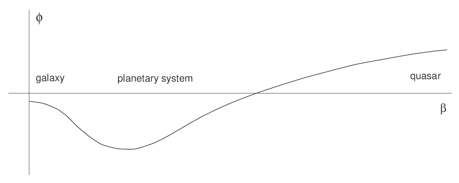
However, one can propose other functions with the desired properties, and it is by combined theoretical investigations in quantum gravity and by comparison with observations that a reasonable function may be established.
VII Summary
In this paper, we considered the vacuum spherically symmetric problem in the theory of gravity described by action (1), which modifies the Plebański self-dual formulation of general relativity by introducing an additional function . In the spherically symmetric case, the two arguments of the function are not independent, and it becomes a function of only one effective field , defined in (6). The form of the function is to be determined from quantum considerations. Since this problem is not yet solved, in concrete physical applications we have explored several different possibilities of its form.
The basic variables of the theory under consideration are the spin connection one-form and the two-form spinor field , while the Lagrange multiplier field can be thought of as expressible in terms of via the algebraic “metricity” equations. The theory with nontrivial does not distinguish any special metric; however, there arises a conformal class of metrics with respect to which the two-form is self-dual. The existence of such a conformal class enables us to speak about the conformal structure of the solution.
The vacuum spherically symmetric solution has several significant features, and we can summarize our results as follows:
1. For arbitrary , the theory respects the analog of the Birkhoff theorem, i.e., the vacuum spherically symmetric solution is necessarily static and asymptotically describes a space of constat curvature. In our theory, this means the existence of a vector field generating a group of diffeomorphisms that leave invariant the fields , and . In the coordinate language, the components of these fields do not depend on the “time” coordinate . This property is probably connected with the fact that our modifications of the Plebański formulation of the general-relativistic action does not increase the order of differential equations. A similar property was recently proved for metric theories which preserve the second-order character of field equations Lovelock.
2. In any domain of its argument in which the function varies slowly (), it acts simply as a (multiple of) the cosmological constant, and the solution in the corresponding spatial domain possesses approximate “metricity” property in the sense that the three components of the self-dual spinor two-form are expressible as self-dual parts of the canonical exterior products of some basis one-forms. These basis one-forms then define a unique metric in the corresponding space-time region, which is an approximate solution of the vacuum Einstein equations. In our spherically symmetric solution, such a behavior is obtained at spatial infinity, where we recover the Schwarzschild metric with small and rapidly decaying “nonmetric” corrections. The value of in this case plays the role of Weyl curvature.
3. If several regions exist in the domain of where the function is slowly varying, then the distinguished metric in the corresponding spatial regions is described by the Schwarzschild-de Sitter form but with different values of the Schwarzschild radius and effective cosmological constant. In other words, the gravitational and cosmological constants become curvature-dependent in this theory. This property of the solution can potentially be used to account for the problem of missing mass in spiral galaxies and other astrophysical objects. The nonmetric corrections in the regions close to the gravitating bodies in this case could also explain the observed anomaly in the acceleration of the Pioneer spacecraft.
4. In addition to this effective remormalization of gravitational and cosmological constants, there arises a nontrivial universal redshift factor between regions of different Weyl curvature . This effect potentially can explain the high redshift of quasars and gamma-ray bursts.
5. The conformal structure of our solution inside the black-hole region is different from that of the Schwarzschild solution and depends on the form of the function . Typically, “inside” the analog of the Schwarzschild horizon one finds another surface of extreme “non-metricity”. This surface is spacelike, and replaces the usual spacelike singularity inside the Schwarzschild black hole. The metric ceases to exist at this surface, but all the dynamical fields of the theory are finite. Thus, this surface is only a metric singularity, but not a singularity of the theory. Across this surface, the coordinates change their spacetime roles once more, and one typically finds another Schwarzschild-like horizon behind this “non-metricity” surface. The theory does not admit arbitrarily small black holes: for small objects, the curvature on the would-be horizon is so strong that non-metric modifications prevent the horizon from being formed. Instead of horizon, one has “naked” hypersurface of non-metricity in this case. The details of the conformal diagram depend on the specific shape of the function . For a simple choice , it is shown in Fig. 1.
Acknowledgments
The authors are grateful to Martín López-Corredoira and Jayant Narlikar for correspondence and to Oleg Barabash for discussion. This work was done at the Perimeter Institute for Theoretical Physics, whose support the authors acknowledge. K. K. was partially supported by an EPSRC advanced fellowship, and Yu. S. was supported by grant No. 5-20 of the “Cosmomicrophysics” programme and by the Program of Fundamental Research of the Physics and Astronomy Division of the National Academy of Sciences of Ukraine, by grant No. F16-457-2007 of the State Foundation of Fundamental Research of Ukraine, by the PPARC grant, and by the INTAS grant No. 05-1000008-7865.
Appendix A Proof of the static property of the metric
In this appendix, we give the details of the proof of static property of the solution to the vacuum spherically symmetric problem.
The most general spherically symmetric expression for the two-form is given by (14):
| (92) |
with the one-forms , , , and given by (16):
| (93) |
Now the functions , , , and are not assumed to be time-independent, but are functions of both and . We are going to show that is a constant (coordinate-independent), and , , and are time-independent due to the field equations.
The expressions for are now modified because of the appearance of time derivatives, so that instead of (20), we have
| (94) |
where overdot denotes the time derivative. Formulas (22) are then modified as follows:
| (95) |
the rest of the projections being zero. Then, using formulas (25) and (26), which remain unchanged, we obtain
| (96) |
where we made the notation
| (97) |
Now we have to compute the left-hand sides of equations (31) and equate them to zero. Computing the component of any of the first two equations in (31), we immediately obtain that , which, in turn, simplifies the expressions (96). Calculating then the and components of the first equation in (31), we get
| (98) |
respectively. The condition is excluded because it contradicts the component of the same equation, which contains a generically nonzero expression . Therefore, one must have .
The remaining four equations stemming from the first two equations in (31) read
| (99) |
where , as usual. Now, subtracting the first equation from the third one, and the second from the fourth one, we obtain, respectively,
| (100) |
which implies
| (101) |
These two equations are equivalent in view of the condition and definition (97).
Under condition (101), the remaining two equations stemming from (99) are precisely equations (32), while the last equation in (31) leads to the two equations (33). Thus, we have the system of differential equations (35). The second equation in (35) then implies that does not depend on time, hence, by virtue of (15), is also time-independent. Finally, the third equation in (35) implies that can only have a time-dependent overall factor, which can always be rescaled to a constant by changing the time variable. This completes the proof of the static property of the spherically symmetric vacuum solution in the theory under investigation.
Appendix B Mass renormalization and redshift: general analysis
In this appendix, we generalize the examples considered in Sec. V. Thus, assume that two regions are characterized by the conditions and , respectively, where is some length scale. We will find the approximate solutions in these regions assuming the behavior
| (102) |
where the variable , and , , and are different constants.
At small radial distances, where , we integrate equations (42) to obtain
| (103) |
We also have
| (104) |
Collecting all the terms, we obtain the leading contribution to the coefficient in metric (18):
| (105) |
where is the value of the effective Schwarzschild radius at small distances, is the value of the function at infinity. We have also assumed the condition , which guarantees that some terms that are of lower power in are actually subleading. This expression is valid if . In the interesting case , the correction to the Schwarzschild–de Sitter metric will also have logarithmic terms; see our concrete example (64) in Sec. V.
As we discussed above, the physical metric can be specified by an additional conformal factor, in which case, we obtain somewhat different corrections. Thus, for the Urbantke metric defined in (52) and for the “volume” metric defined in (54), we will have the coinciding approximate relations for :
| (106) |
At large radial distances, where , we have
| (107) |
| (108) |
In this case, we obtain the following leading contribution to the metric:
| (109) |
where , and
| (110) |
In the case of extra conformal factors, again, the corrections to the Schwarzschild-de Sitter metric will be somewhat different. For the Urbantke metric defined in (52) and for the “volume” metric defined in (54), we have the same approximate relations for :
| (111) |
We note that in our approximation in these regions, so the physical metric is well defined. The contributions proportional to and in (105), (106) and (109), (111), respectively, are small and can be dropped if the constants and are not very large. However, these contributions themselves are of the same order as the “nonmetricity.” Their physical interpretation, therefore, requires the knowledge of the matter couplings in our theory, which is an issue still to be resolved.
For , the observed gravitational mass of the central object at large distances is times larger than it is at small distances. In the intermediate region of radial distances
| (112) |
the metric coefficient behaves in a complicated way; moreover, the physical metric may not be well defined in this region at all. If several regions exist in the space of in which , then obvious renormalizations of the observed gravitational masses and redshift factors exist between these regions.
References
- (1) K. Krasnov, “Renormalizable Non-Metric Quantum Gravity?” arXiv:hep-th/0611182.
- (2) K. Krasnov, “Non-Metric Gravity I: Field Equations,” arXiv:gr-qc/0703002.
- (3) J. Plebański, “On the separation of Einsteinian substructures,” J. Math. Phys. 18, 2511 (1977).
- (4) I. Bengtsson, “Note on non-metric gravity,” Mod. Phys. Lett. A 22, 1643 (2007) [arXiv:gr-qc/0703114].
- (5) R. Capovilla, J. Dell, T. Jacobson, and L. Mason, “Self-dual 2-forms and gravity,” Class. Quantum Grav. 8, 41 (1991).
- (6) O. Brodbeck, “On symmetric gauge fields for arbitrary gauge and symmetry groups,” Helv. Phys. Acta 69, 321 (1996) [arXiv:gr-qc/9610024].
- (7) H. Urbantke, J. Math. Phys. 25, 2321 (1983).
- (8) J. R. Brownstein and J. W. Moffat, “Galaxy Rotation Curves Without Non-Baryonic Dark Matter,” Astrophys. J. 636, 721 (2006) [arXiv:astro-ph/0506370]; J. R. Brownstein and J. W. Moffat, “Galaxy Cluster Masses Without Non-Baryonic Dark Matter,” Mon. Not. Roy. Astron. Soc. 367 527 (2006) [arXiv:astro-ph/0507222]; J. R. Brownstein and J. W. Moffat, “The Bullet Cluster 1E0657-558 evidence shows Modifed Gravity in the absence of Dark Matter,” arXiv:astro-ph/0702146.
- (9) J. D. Anderson, P. A. Laing, E. L. Lau, A. S. Liu, M. M. Nieto, and S. G. Turyshev, “Indication, from Pioneer 10/11, Galileo, and Ulysses Data, of an Apparent Anomalous, Weak, Long-Range Acceleration,” Phys. Rev. Lett. 81, 2858 (1998) [arXiv:gr-qc/9808081]; J. D. Anderson, P. A. Laing, E. L. Lau, A. S. Liu, M. M. Nieto, and S. G. Turyshev, “Study of the anomalous acceleration of Pioneer 10 and 11,” Phys. Rev. D 65, 082004 (2002) [arXiv:gr-qc/0104064]; C. B. Markwardt, “Independent confirmation of the Pioneer 10 anomalous acceleration,” arXiv:gr-qc/0208046; S. G. Turyshev, V. T. Toth, L. R. Kellogg, E. L. Lau, and K. J. Lee, “The Study of the Pioneer Anomaly: New Data and Objectives for New Investigation,” Int. J. Mod. Phys. D 15, 1 (2006) [arXiv:gr-qc/0512121].
- (10) R. H. Sanders, “Solar system constraints on multi-field theories of modified dynamics,” Mon. Not. Roy. Astron. Soc. 370, 1519 (2006) [arXiv:astro-ph/0602161].
- (11) H. C. Arp, Seeing Red: Redshifts, Cosmology and Academic Science, Apeiron, Montreal (1998); J. V. Narlikar, “Noncosmological Redshifts,” Space Science Reviews 50, 523 (1989); G. R. Burbidge, “Noncosmological Redshifts,” Publ. Astr. Soc. Pacific 113, 899 (2001).
- (12) M. López-Corredoira, “Observational Cosmology: caveats and open questions in the standard model,” Recent. Res. Devel. Astron. Astrophys. 1, 561 (2003), arXiv:astro-ph/0310214; M. López-Corredoira and C. M. Gutiérrez, “Research on candidates for non-cosmological redshifts,” in: “First Crisis In Cosmology Conference, CCC-1” [AIP Conf. Proc., 822(1)], ed. by J. B. Almeida and E. J. Lerner, pp. 75–92, arXiv:astro-ph/0509630.
- (13) S. Collin, “Quasars and Galactic Nuclei, a Half-Century Agitated Story,” arXiv:astro-ph/0604560.
- (14) G. R. Burbidge, “The Sources of Gamma-Ray Bursts and Their Connections with QSOs and Active Galaxies,” Astrophys. J. 585, 112 (2003); G. R. Burbidge, “Connections between Gamma-Ray Bursts, QSOs and active galaxies,” in: Proceedings of the 2nd BeppoSAX Conference: The Restless High-Energy Universe, Nucl. Phys. B – Proceedings Supplements 132, 305 (2004).
- (15) J. L. Greenstein and M. Schmidt, “The Quasi-Stellar Radio Sources 3C 48 and 3C 273,” Astrophys. J. 140, 1 (1964).
- (16) C. Charmousis and J.-F. Dufaux, “General Gauss-Bonnet brane cosmology,” Class. Quantum Grav. 19, 4671 (2002) [arXiv:hep-th/0202107]; R. Zegers, “Birkhoff’s theorem in Lovelock gravity,” J. Math. Phys. 46, 072502 (2005) [arXiv:gr-qc/0505016]; S. Deser and J. Franklin, “Birkhoff for Lovelock Redux,” Class. Quantum Grav. 22, L103 (2005) [arXiv:gr-qc/0506014].