Energy of zeros of random sections on Riemann SurfaceThanks: The author would like to thank his advisor Prof. Zelditch for his helpful suggestion on this work. He also wants to thank Jian Kong and Brain Macdonald for their help on computer program.

Qi Zhong Address: Department of Mathematics, Johns Hopkins University, USA, 21218 Email address: qzhong@math.jhu.edu

Abstract.

The purpose of this paper is to determine the asymptotic of the average energy of a configuration of $N$ zeros of system of random polynomials of degree $N$ as $N\to\infty$ and more generally the zeros of random holomorphic sections of a line bundle $L\to M$ over any Riemann surface. And we compare our results to the well-known minimum of energies.

1. Introduction

This article is concerned with the asymptotic of the average energy of the configuration of zeros of $N$ -degree random polynomials as $N\to\infty$ and more generally the zeros of random holomorphic sections of a line bundle $L\to M$ over any compact Riemann surface without boundary. The energy of a configuration of points $\{z_{1},\dots,z_{N}\}$ on a surface $M$ equipped with a Riemannian metric $g$ is defined by

\mathcal{E}^{N}_{G_{g}}=\sum_{i\neq j}G_{g}(z_{i},z_{j}),

(1)

where $G_{g}$ is the Green’s function for $g$ , $G_{g}(z,w)=-\frac{1}{2\pi}\chi(z,w)\log r_{g}(z,w)+F(z,w)$ ,where $F\in C^{\infty}(M\times M)$ and $\chi(z,w)$ is the cut-off function near the diagonal, we will discuss the notations in §2.5 ; other energies will also be studied. Electrons moving freely on the surface distribute themselves in a minimal energy configuration, and many articles have been devoted to finding the minimal energy configurations and the asymptotic of the minimal energy.

The question studied in this article is the extent to which zeros of random polynomials of degree $N$ tend to resemble minimal energy configurations of N points. Zeros of random polynomials in complex dimension one repel and like minimal energy configurations tend to stay $1/\sqrt{N}$ apart. Our main results show that the average energy of such random zeros is of the same order of magnitude as that of minimal energy configurations.

To state our results, we need some notation. Throughout the article we identify polynomials of degree $N$ with holomorphic sections $H^{0}({\mathbb{C}}{\mathbb{P}}^{1},\mathcal{O}(N))$ of the $N$ th power of the hyperplane section bundle over the complex projective line ${\mathbb{C}}{\mathbb{P}}^{1}$ . Our methods apply equally to holomorphic sections $H^{0}(M,L^{N})$ of powers of a positive holomorphic line bundle $L\to M$ over any compact Riemann surface.Thus, in addition to studying zeros of polynomials, we study zeros of random theta functions over a Riemann surface of genus one, and zeros of random holomorphic k-differentials over a surface of higher genus. Moreover, our results apply to general k $\ddot{a}$ hler metrics $g$ on these Riemann surfaces.

As recalled in $\lx@sectionsign 2.1$ , a choice of hermitian metric on L determines an inner product on $H^{0}(M,L^{N})$ and then a Gaussian measure $\mu_{h^{N}}$ on this spaces. Roughly speaking, a random section $S_{c}$ is expressed in terms of an orthonormal basis $S_{j}$ of $H^{0}(M,L^{N})$ as $S_{c}=\sum c_{j}S_{j}$ where the $c_{j}$ are independent complex normal Gaussian random variables. Also we define Riemannian form $dV_{M}=\omega_{h}=\frac{i}{2}\Theta_{h}$ . The metric $g$ defining Green’s function is not necessarily equal to the metric derived by $h$ .

In the case of ${\mathbb{C}}{\mathbb{P}}^{1}$ , we also consider the energies $\mathcal{E}_{s}$ defined by

\mathcal{E}_{s}(z_{1},\dots,z_{N})=\sum_{i\not=j}\frac{1}{[z_{i},z_{j}]^{s}}.

(2)

In the case $s=0$ , the $s$ -energy is defined to be the logarithmic energy

\mathcal{E}_{0}(z_{1},\dots,z_{N})=\sum_{i\not=j}-\log[z_{i},z_{j}].

(3)

Here $[z,w]$ is the chordal distance between two points on $S^{2}$ , where $z$ and $w$ are the two points on ${\mathbb{C}}{\mathbb{P}}^{1}$ corresponding to some points on $S^{2}$ . If $r$ is the round distance on $S^{2}$ , then the relation between $[\cdot,\cdot]$ and $r$ is

[a,b]=\sqrt{2(1-\cos r(a,b))}

(4)

here, $a$ , $b$ are points on $S^{2}$ .

We define ${\mathbf{E}}\mathcal{E}^{N}_{G_{g}}$ to be the expected (average) value of the energy of the zeros of Gaussian random sections chosen from the ensemble $(H^{0}(M,L^{N}),\mu_{h})$ by

{\mathbf{E}}\mathcal{E}^{N}_{G_{g}}=\int_{H^{0}(M,L^{N})}\mathcal{E}_{G_{g}}(Z_{s})d\mu_{h}(s)=\int_{{\mathbb{C}}^{d_{N}}}\mathcal{E}_{G_{g}}(Z_{s})\frac{e^{-|c|^{2}}}{\pi^{d_{N}}}dc,

(5)

here

\mathcal{E}_{G_{g}}(Z_{s})=\mathcal{E}_{G_{g}}(z_{1},\dots,z_{N})=\sum_{\begin{subarray}{c}z_{i}\neq z_{j}\\ z_{i},z_{j}\in Z_{s}\end{subarray}}{G_{g}}(z_{i},z_{j})

where $Z_{s}=\{z_{1},\dots,z_{N}\}$ is the zeros of $s$ and $d_{N}=\dim H^{0}(M,L^{N})$ .

Note that if $s$ has a double zero, the energy is infinite, but this occurs with measure zero.

Recall a Green’s function $G_{g}$ on compact Riemann Manifold $(M,g)$ without boundary is the kernel of $-\Delta^{-1}_{g}$ . Then the expected (average) energy is satisfies:

Theorem 1.1.

Let $(L,h)\to M$ be a positive Hermitian line bundle on $M$ with $\frac{i}{2}\Theta_{h}=\omega$ , $\Theta$ is the curvature form and $\omega$ gives $M$ a Riemannian volume form. We assume the Chern class of $L$ , $c_{1}(L)=1$ . Then the expected average of Green’s function energy of zeros of random sections is given by:

{\mathbf{E}}\mathcal{E}^{N}_{G_{g}}=-\frac{1}{4\pi}N\log N+O(N).

(6)

Remark: If $c_{1}(L)\neq 1$ , then the number of zeros is $c_{1}(L)\cdot N.$

In [Hr], Elkies proved that

\sum_{i\neq j}g_{v}(z_{j},z_{k})\leq\frac{1}{2}N\log N+\frac{11}{3}N+o(N).

where $g_{v}$ is the Green’s function with respected to a special volume form $d\mu_{v}$ see [Hr]. We notice that Elkies’ normalization of Green’s function is

g_{v}(z,w)=\log{|z,w|_{v}}+F^{\prime}(z,w)

which is negative near the diagonal. While, our normalization for Green’s function

G_{g}(z,w)=-\frac{1}{2\pi}\chi(z,w)\log r_{g}(z,w)+F(z,w)

is positive near the diagonal. Then we can rewrite Elkies’ result

(-\frac{1}{2\pi}\sum_{i\neq j}g_{v}(z_{i},z_{j}))\geq-\frac{1}{4\pi}N\log N-\frac{11}{6\pi}N+o(N)

(7)

Remark:

(1)

We see that the leading order term in equation (7) is the same as the one in equation (6). It means that the probability that the energy is above the minimum goes to zero as $N\to\infty$ , i.e.

P(s:\mathcal{E}_{G_{g}}(s)\leq a+\epsilon N\log N)\leq\frac{o(N)}{\epsilon},

where $a=-\frac{1}{4\pi}N\log N-\frac{11}{6\pi}N+o(N)$ which is the minimum of the energy. Above formula is not hard to verify. If $a=\inf_{s}\mathcal{E}_{G_{g}}(s)$ and $MAX=\sup_{s}\mathcal{E}_{G_{g}}(s)$ , then we get

	$\displaystyle a+o(N)a=$	$\displaystyle\int_{H^{0}(M,L^{N})}\mathcal{E}_{G_{g}}(Z_{s})d\mu_{h}(s)$
	$\displaystyle=$	$\displaystyle\int^{MAX}_{a}Xd\mu_{\mathcal{E}_{G_{g}}(s)}$
	$\displaystyle=$	$\displaystyle\int^{a+\epsilon a}_{a}Xd\mu_{\mathcal{E}_{G_{g}}(s)}+\int^{MAX}_{a+\epsilon a}Xd\mu_{\mathcal{E}_{G_{g}}(s)}$
	$\displaystyle\geq$	$\displaystyle a\cdot(1-\mu(s:\mathcal{E}_{G_{g}}(s)\geq a+\epsilon a))+(a+\epsilon a)\cdot\mu(s:\mathcal{E}_{G_{g}}(s)\geq a+\epsilon a)$
	$\displaystyle=$	$\displaystyle a+\epsilon a\cdot\mu(s:\mathcal{E}_{G_{g}}(s)\geq a+\epsilon a)$

So we have $\mu(s:\mathcal{E}_{G_{g}}(s)\geq a+\epsilon a)\leq\frac{o(N)}{\epsilon}.$

(2)

Our expect average of Green’s function energy is scale metric invariant,that is, if we rescale the metric $g\to rg$ , then our result (6) doesn’t change. When $g\to rg$ , $\Delta_{g}$ operator becomes $\frac{1}{r}\Delta_{g}$ , as we discuss in §2.5, $G_{g}(z,w)$ is the kernel of $(-\Delta^{-1})$ , then $G_{g}(z,w)dV_{g}\to rG_{g}(z,w)dV_{g}$ as $g\to rg$ . On the other side, $dV_{g}\to rdV_{g}$ as $g\to rg$ , therefore, $G_{g}(z,w)$ doesn’t change as $g\to rg$ .
(3)

The leading term order term is independent of $g$ and $h$ .
(4)

We define the Green’s function $G$ to be positive near the diagonal and the average is negative. Then we conclude that the off diagonal part dominates the energy.

Theorem 1.2.

(1)

Consider ${\mathbb{C}}{\mathbb{P}}^{1}$ with the Fubini-Study metric $g$ , let $(L,h)\to{\mathbb{C}}{\mathbb{P}}^{1}$ be a positive Hermitian line bundle on ${\mathbb{C}}{\mathbb{P}}^{1}$ with $\frac{i}{2}\Theta_{h}=\omega_{g}$ , $\Theta$ is the curvature form. we recall equation (2) and have expected s-energy:

•

when $s=2$

	$\displaystyle{\mathbf{E}}\mathcal{E}^{N}_{2}=$	$\displaystyle\frac{1}{4}{N^{2}}\log N+\frac{3N^{2}}{4}\log(\log N)+\frac{N^{2}}{2}\log 2+\frac{1}{2}N^{2}(\frac{M}{L})^{2}$
		$\displaystyle-2N^{2}\log\frac{M}{L}+o(N^{2}).$		(8)

•

When $s<2$

{\mathbf{E}}\mathcal{E}^{N}_{s<2}=\frac{2^{1-s}}{2-s}N^{2}+\frac{1}{(2(2-s))}N^{1+\frac{s}{2}}(\log N)^{1-\frac{s}{2}}+o(N^{1+\frac{s}{2}}(\log N)^{1-\frac{s}{2}})

(9)

•

When $2<s<4$

${\mathbf{E}}\mathcal{E}^{N}_{2<s<4}=C\frac{N^{1+\frac{s}{2}}}{4-s}+O(N^{1+\frac{s}{2}}(\log N)^{1-\frac{s}{2}}).$ (10)

We will discuss the constant $C$ in the remark at the end of this section.

(2)

Under the same condition as above,we recall equation (3) and have expected logarithmic energy:

	$\displaystyle{\mathbf{E}}\mathcal{E}^{N}_{0}=$	$\displaystyle-(\log 2-\frac{1}{2})N^{2}+\frac{N}{2}\log^{2}N-\frac{1}{2}N\log(\log N)\log N$
		$\displaystyle+\frac{1}{2}N\log N+\frac{1}{2}(\log 2+1)N+o(N).$		(11)

Let us compare our results on average energy to the prior results on minimal energy. For $s-$ energy case, Saff-Kuijilaars in [KS] identified ${\mathbb{C}}{\mathbb{P}}^{1}$ as $S^{2}\in{\mathbb{R}}^{3}$ and considered the energy

\mathcal{E}^{\prime}_{s}(x_{1},\dots,x_{N})=\sum_{i<j}\frac{1}{|x_{i}-x_{j}|^{s}}

where $x_{i}$ are the points on $S^{2}\subset{\mathbb{R}}^{3}$ not on ${\mathbb{C}}{\mathbb{P}}^{1}$ and $|x-y|$ is the chordal distance of $S^{2}$ . They investigated the energy $\mathcal{E}^{\prime}_{s}$ . Moreover, they define the minimal $s-$ energy for $N$ points on the sphere

E_{s}(N):=\min_{\{x_{1},...,x_{N}\}}\{\mathcal{E}^{\prime}_{s}\}.

It was proved by Saff-Kuijlaars that when $s=2$ , then

{}E_{2}(S^{2},N)\sim\frac{1}{8}\;N^{2}\log N.

(12)

And when $s>2$ , then

C_{1}N^{1+s/2}\leq E_{s}(N)\leq C_{2}N^{1+s/2},

(13)

$C_{1},C_{2}>0$ . And when $s<2$ , then

{}E_{2}(S^{2},N)\leq\frac{1}{2}V_{2}(s)N^{2}-CN^{1+\frac{s}{2}},

(14)

here, $C>0$ and $V_{2}(s)=\frac{\Gamma(\frac{3}{2})\Gamma(2-s)}{\Gamma((2-s+1)/2)\Gamma(2-\frac{s}{2})}$ .

B.Bergersen, D. Boal and P. Palffy-Muboray in [BBP] identified ${\mathbb{C}}{\mathbb{P}}^{1}$ as $S^{2}\in{\mathbb{R}}^{3}$ and considered the energy

\mathcal{E}^{\prime}_{0}(x_{1},\dots,x_{N})=\sum_{i<j}-\log|x_{i}-x_{j}|.

They investigated the ground-state energy of the logarithm energy of $N$ points $\{x_{1},...,x_{N}\}$ , which is the minimal energy of $\mathcal{E}^{\prime}_{0}$ for large $N$ :

\min_{\{x_{1},...,x_{N}\}}\{\mathcal{E}^{\prime}_{0}\}=-(\frac{1}{2}\log 2-\frac{1}{4})N^{2}-\frac{N}{4}\log N+\cdots^{1}

(15)

¹¹footnotetext: We use

E_{o}

to consist our notation, in [BBP], they defined their own notation.

And in that paper, they gave a formula for the ground-state energy $E$

Remark:

•

Our $s-$ energy is twice of the $s-$ energy in [KS], $\mathcal{E}_{s}=2\mathcal{E}^{\prime}_{s}$ . So by the equations (• ‣ 1) and (12), we see that when $s=2$ the leading order term of the expected average of energy is the same as the one in minimum energy. So is the 0-energy case.
•

In equation (10), we can’t figure out the constant precisely. Actually it is a conjecture in [KS]. Since in the Green’s function energy, 2-energy and 0-energy, all the leading order terms of expected average are the same as the one in minimum energy, this paper probably offers a method to solve the conjecture. It will be discussed more after the proof of Theorem 1.2(1).

An additional motivation to study energies of random zeros is that there are examples of numerical integration over the Riemann surface. In numerical integration, one integrates a function with respect to a probability measure $\mu$ by generation $N$ random points from the ensemble $(M,\mu)$ and averaging over the points. In this article, we generate N random points from $(M,\omega_{h})$ by taking the zeros of a random polynomial. The same numerical integration procedure is used in the recent paper [DKLR] to numerically integrate quantities over Calabi-Yau threefolds. The more elementary numerical integrations in this article illustrate the speed of convergence of the integration procedure.

2. Background

We begin with some notations and basic properties of sections of holomorphic line bundles, Gaussian measures and the relation between polynomials and sections. The notations are the same as in [SZ1] and [BSZ]. Here we only deal with complex dimension one case, and [PBZ] discuss the general case.

2.1. Complex Geometry.

We denote by $(L,h)\to M$ a holomorphic line bundle with smooth Hermitian metric $h$ whose curvature form

\Theta_{h}=-\partial\bar{\partial}\log||e_{L}||^{2}_{h},

(16)

is a positive $(1,1)$ -form. Here, $e_{L}$ is a local non-vanishing holomorphic section of $L$ over an open set $U\subset M$ , and $||e_{L}||_{h}=h(e_{L},e_{L})^{1/2}$ is the $h-$ norm of $e_{L}$ . As in [BSZ], we give $M$ the Hermitian metric corresponding to the K $\ddot{a}$ hler form $\omega=\frac{\sqrt{-1}}{2}\Theta_{h}$ and the induced Riemannian volume form

dV_{M}=\omega.

(17)

We denote by $H^{0}(M,L^{N})$ the space of holomorphic sections of $L^{N}=L\otimes\cdots\otimes L.$ The metric $h$ induces Hermitian metrics $h^{N}$ on $L^{N}$ given by $||s^{\otimes N}||_{h^{N}}=||s||^{N}_{h}.$ We give $H^{0}(M,L^{N})$ the Hermitian inner product

<s_{1},s_{2}>=\int_{M}h^{N}(s_{1},s_{2})dV_{M}\ \ \ \ (s_{1},s_{2}\in H^{0}(M,L^{N})),

(18)

and we write $|s|=<s,s>^{1/2}.$

For a holomorphic section $s\in H^{0}(M,L^{N})$ , we let $Z_{s}$ denote the current of integration over the zero divisor of $s$ :

(Z_{s},\varphi)=\int_{Z_{s}}\varphi,\ \ \ \varphi\in\mathcal{D}^{0,0}(M),

here $\mathcal{D}^{0,0}(\Omega)$ compactly supported $(0,0)$ forms (compactly supported smooth function) on M. A current is an element of the dual space $\mathcal{D}^{0,0}(M)^{\prime}.$

The Poincar $\acute{e}$ -Lelong formula (see e.g. [GH]) expresses the integration current of a holomorphic section $s=ge^{\otimes N}_{L}$ in the form:

Z_{s}=\frac{i}{\pi}\partial\bar{\partial}\log|g|=\frac{i}{\pi}\partial\bar{\partial}\log||s||_{h^{N}}+N\omega.

(19)

We also denote by $|Z_{s}|$ the Riemannian $0-$ volume i.e. Riemannian function along the regular points of $Z_{s}$ , regarded as a measure on $M$ :

(|Z_{s}|,\varphi)=\int_{Z^{reg}_{s}}\varphi dVol;

(20)

2.2. Random sections and Gaussian measures.

We now give $H^{0}(M,L^{N})$ the complex Gaussian probability measure

d\mu(s)=\frac{1}{\pi^{d_{N}}}e^{-|c|^{2}}dc,\ \ s=\sum^{d_{N}}_{j=1}c_{j}S^{N}_{j},

(21)

where $\{S^{N}_{j}:1\leq j\leq d_{N}\}$ is an orthonormal basis for $H^{0}(M,L^{N})$ and $dc$ is $2d_{N}-$ dimensional Lebesgue measure. This Gaussian is characterized by the property that the $2d_{N}$ real variable $\mathcal{R}c_{j}$ , $\mathcal{I}c_{j}$ ( $j=1,....,d_{N}$ ) are independent random variables with mean 0 and variance $\frac{1}{2}$ ;i.e.,

\mathbf{E}c_{j}=0,\ \ \mathbf{E}c_{j}c_{k}=0,\ \ \mathbf{E}c_{j}\bar{c}_{k}=\delta_{jk}.

Here and throughout this article, $\mathbf{E}$ denotes expectation: $\mathbf{E}\varphi=\int\varphi d\mu$ .

We then regard the currents $Z_{s}$ (resp. measures $|Z_{s}|$ ), as current-valued (resp. measure-valued) random variables n the probability space ( $H^{0}(M,L^{N}),d\mu$ );i.e., for each test form (resp. function) $\varphi$ , ( $|Z_{s}|,\varphi$ ) (resp. ( $|Z_{s}|,\varphi$ )) is a complex-valued random variable.

Since the zero current $Z_{s}$ is unchanged when $s$ is multiplied by an element of ${\mathbb{C}}^{*}$ , our results are the same if we instead regard $Z_{s}$ as a random variable on the unit sphere $SH^{0}(M,L^{N})$ with Haar probability measure. We prefer to use Gaussian measures in order to facilitate computations.

2.3. Correlation currents and measures.

The $n-$ point correlation current of the zeros is the current on $M^{n}=M\times M\times...\times M$ ( $n$ times) given by

K^{N}_{n}(z^{1},...,z^{n}):=\mathbf{E}(Z_{s}(z^{1})\otimes Z_{s}(z^{2})\otimes\cdots\otimes Z_{s}(z^{n}))

(22)

in sense that for any test form $\varphi_{1}(z^{1})\otimes\cdots\otimes\varphi_{n}(z^{n})\in\mathcal{D}^{0,0}(M)\otimes\cdots\otimes\mathcal{D}^{0,0}(M).$

(K^{N}_{n}(z^{1},...,z^{n}),\varphi_{1}(z^{1})\otimes\cdots\varphi_{n}(z^{n}))=\mathbf{E}[(Z_{s},\varphi_{1})(Z_{s},\varphi_{2})\cdots(Z_{s},\varphi_{n})].

(23)

When $n=2$ , the correlation measures take the form

K^{N}_{2}(z,w)=[\Delta]\wedge(K^{N}_{1}(z)\otimes 1)+\kappa^{N}(z,w)\omega_{z}\otimes\omega_{w}\ \ \ (N>>0),

(24)

where $[\Delta]$ denotes the current of integration along the diagonal $\Delta={(z,z)}\subset M\times M$ , and $\kappa^{N}\in C^{\infty}(M\times M)$ . In [SZ3], Bernard Shiffman and Steve Zelditch introduced a primary object ”bipotential” for the pair correlation current; in terms of the notation used here, the bipotential is a function $Q_{N}(z,w)$ such that:

\Delta_{z}\Delta_{w}Q_{N}(z,w)=K^{N}_{2}(z,w)-K^{N}_{1}(z)\wedge K^{N}_{1}(w).

(25)

In [SZ3], the authors proved that for $b>\sqrt{j+2k}$ , $j,k\geq 0$ , we have

\nabla^{j}Q_{N}(z,w)=O(N^{-k})\ \ \ \ uniformly\ for\ r_{h}(z,w)\geq b\sqrt{\frac{\log N}{N}},

(26)

here $\nabla^{j}R={\frac{\partial^{j}R}{\partial u^{K^{\prime}}\partial u^{K"}}}:|K^{\prime}|+|K"|=j$ , and $r_{h}$ is the geodesic distance derived by $h$ . As (25), we have

K^{N}_{2}(z,w)-K^{N}_{1}(z)\wedge K^{N}_{1}(w)=O(N^{-k})\ \ \ \ uniformly\ for\ r_{h}(z,w)\geq b\sqrt{\frac{\log N}{N}}.

(27)

2.4. Relation of polynomials and sections.

By homogenizing, we may identify the space of polynomials of degree $N$ in one complex variables with the space $H^{0}({\mathbb{C}}{\mathbb{P}}^{1},\mathcal{O}(N))$ of holomorphic sections of the $N-$ power of the hyperplane bundle over ${\mathbb{C}}{\mathbb{P}}^{1}$ . This space carries a natural $SU(2)$ -invariant inner product and associated Gaussian measure $d\mu$ . We associate degree $N$ polynomial $p$ zero set $Z_{p}=\{p(z)=0\}$ , which is almost always discrete, and thus obtain a random point process on ${\mathbb{C}}{\mathbb{P}}^{1}$ .

2.5. Green’s function on Riemann surfaces

In this section, we discuss Green’s functions on Riemann surfaces $(M,g)$ . The Green’s function is the kernel of $(-\Delta_{g})^{-1}$ i.e. $G_{g}(z,w)dV_{g}=-\Delta^{-1}$ , which is orthogonal to the constant functions, that is

\int_{M}G_{g}(z,w)dV_{g}=0

(28)

. Here, $-\Delta$ is the Laplacian operator. Let $\varphi_{j}$ be the eigenfunctions of $-\Delta$ , then

G_{g}(z,w)=\sum_{j\neq 0}\frac{\varphi_{j}(z)\varphi_{j}(w)}{\lambda^{2}_{j}},

(29)

where $-\Delta\varphi_{j}=\lambda_{j}\varphi_{j}$ , and $\lambda_{j}=0.$ So

-\Delta G_{g}(z,w)=\sum_{j\neq 0}\varphi_{j}(z)\varphi_{j}(w)=\delta_{z}(w)-\frac{1}{vol(M,g)}.

(30)

It is well-known that $G_{g}(z,w)$ on Riemann surface has following formula [see H]

G_{g}(z,w)\sim-\frac{1}{2\pi}\chi(z,w)\log r(z,w)+F(z,w)

(31)

here, $F\in C^{\infty}(M\times M)$ and $\chi(z,w)$ is a cut-off function which equals 1 on $r(z,w)\leq C_{1}$ and 0 on $r(z,w)\geq C_{2}$ , where $0<C_{1}<C_{2}$ .

3. Proof of Theorem 1.1

Lemma 3.1.

$\int_{M\times M}G_{g}(z,w)K_{1}^{N}(z)\wedge K_{1}^{N}(w)=O(N^{-2})$

Proof.

In [SZ3], the authors proved that

K^{N}_{1}(z)=\frac{i}{\pi}\partial\bar{\partial}\log\Pi_{N}(z,z)+\frac{N}{\pi}\omega_{z},

(32)

where, $\Pi_{N}(z,z)$ is the Szegö kernel, we have following asymptotic:

\Pi_{N}(z,z)=N(1+\frac{s(z)}{N}+O(N^{-2})),

(33)

where $s(z)$ is the scalar curvature of $\omega_{z}$ . So we get

\log\Pi_{N}(z,z)=\log(N(1+\frac{s(z)}{N}+O(N^{-2}))=\log N+\frac{s(z)}{N}+O(N^{-2})

(34)

and

K^{N}_{1}(z)=\frac{N}{\pi}\omega_{z}+\frac{i}{\pi N}\partial\bar{\partial}s(z)+O(N^{-2})

(35)

		$\displaystyle\int_{M\times M}G_{g}(z,w)K_{1}^{N}(z)\wedge K_{1}^{N}(w)$
	$\displaystyle=$	$\displaystyle\int_{M\times M}G_{g}(z,w)(\frac{N}{\pi}\omega_{z}+\frac{i}{\pi N}\partial\bar{\partial}s(z)+O(N^{-2}))\wedge(\frac{N}{\pi}\omega_{w}+\frac{i}{\pi N}\partial\bar{\partial}s(w)+O(N^{-2}))$

Since $\int_{M}G_{g}(z,w)\omega_{z}=0$ , the last term in above equations becomes

		$\displaystyle\int_{M\times M}G_{g}(z,w)(\frac{N}{\pi}\omega_{z}+\frac{i}{\pi N}\partial\bar{\partial}s(z)+O(N^{-2}))\wedge(\frac{N}{\pi}\omega_{w}+\frac{i}{\pi N}\partial\bar{\partial}s(w)+O(N^{-2}))$
	$\displaystyle=$	$\displaystyle-\frac{1}{(\pi N)^{2}}\int_{M\times M}G_{g}(z,w)\partial\bar{\partial}s(z)\wedge\partial\bar{\partial}s(w)+o(N^{-2})$

So we have

\int_{M\times M}G_{g}(z,w)K_{1}^{N}(z)\wedge K_{1}^{N}(w)=O(N^{-2}).

∎

Lemma 3.2.

If $w=z+\frac{u}{\sqrt{N}}$ , we have:

{\mathbf{E}}\mathcal{E}^{N}_{G_{g}}=N\int_{M}\int_{|u|\leq b\sqrt{\log N}}G_{g}(z,z+\frac{u}{\sqrt{N}})(H(\frac{1}{2}u^{2})-1)\omega_{z}\otimes\frac{i}{2\pi}|u|^{2}+O(N^{-k}),\;\;\forall k>0,

where $H$ will be given in the proof and $|u|=\sqrt{N}r_{h}(z,w)$ .

Proof.

By equation (4) and our discussion in section 2, we get:

	$\displaystyle{\mathbf{E}}\mathcal{E}^{N}_{G_{g}}$	$\displaystyle=\int_{H^{0}(M,L^{N})}\mathcal{E}_{G_{g}}(Z_{s})d\mu_{h}(s)$
		$\displaystyle={\mathbf{E}}(G_{g}(z,w),Z_{s}\otimes Z_{s}-Z_{\Delta})$
		$\displaystyle=(G_{g}(z,w),K^{N}_{2}(z,w)-[\Delta]\wedge(K^{N}_{1}(z)\otimes 1))$
		$\displaystyle=\int_{M\times M}G_{g}(z,w)(K^{N}_{2}(z,w)-[\Delta]\wedge(K^{N}_{1}(z)\otimes 1))$
		$\displaystyle=\int_{M}\int_{r_{h}(z,w)\leq\frac{b\sqrt{\log N}}{\sqrt{N}}}G_{g}(z,w)K^{N}_{2}(z,w)-[\Delta]\wedge(K^{N}_{1}(z)\otimes 1)$
		$\displaystyle+\int_{M}\int_{r_{h}(z,w)\geq\frac{b\sqrt{\log N}}{\sqrt{N}}}G_{g}(z,w)K^{N}_{2}(z,w)$

By the lemma 3.1, we have:

		$\displaystyle\int_{M}\int_{r_{h}(z,w)\leq\frac{b\sqrt{\log N}}{\sqrt{N}}}G_{g}(z,w)K^{N}_{2}(z,w)-[\Delta]\wedge(K^{N}_{1}(z)\otimes 1)$
		$\displaystyle+\int_{M}\int_{r_{h}(z,w)\geq\frac{b\sqrt{\log N}}{\sqrt{N}}}G_{g}(z,w)K^{N}_{2}(z,w)-\int_{M\times M}G(z,w)K_{1}^{N}(z)\wedge K_{1}^{N}(w)+O(N^{-2})$
		$\displaystyle=\int_{M}\int_{r_{h}(z,w)\leq\frac{b\sqrt{\log N}}{\sqrt{N}}}G_{g}(z,w)(K^{N}_{2}(z,w)-[\Delta]\wedge(K^{N}_{1}(z)\otimes 1)-K_{1}^{N}(z)\wedge K_{1}^{N}(w))$
		$\displaystyle+\int_{M}\int_{r_{h}(z,w)\geq\frac{b\sqrt{\log N}}{\sqrt{N}}}G_{g}(z,w)(K^{N}_{2}(z,w)-K^{N}_{1}(z)\wedge K^{N}_{1}(w))+O(\frac{1}{N^{2}})$

Since $G_{g}(z,w)=-\frac{1}{2\pi}\chi(z,w)\log r_{g}(x,y)+F(z,w)$ and $F$ is bounded since $M$ is compact, therefore when $\ r_{h}(s,w)\geq b\sqrt{\frac{\log N}{N}}$ , then $r_{g}(s,w)\geq b^{\prime}\sqrt{\frac{\log N}{N}}$ , $|G_{g}(z,w)|$ is bounded by $\log N$ , by the equation (26),the last equation becomes:

\int_{M}\int_{r_{h}(z,w)\geq\frac{b\sqrt{\log N}}{\sqrt{N}}}G_{g}(z,w)(K^{N}_{2}(z,w)-K^{N}_{1}(z)\wedge K^{N}_{1}(w))=O(N^{-k}),

so we get

	$\displaystyle{\mathbf{E}}\mathcal{E}^{N}_{G_{g}}=$	$\displaystyle\int_{M}\int_{r_{h}(z,w)\leq\frac{b\sqrt{\log N}}{\sqrt{N}}}G_{g}(z,w)(K^{N}_{2}(z,w)-[\Delta]\wedge(K^{N}_{1}(z)\otimes 1)-K_{1}^{N}(z)\wedge K^{N}_{1}(w))$
		$\displaystyle+O(N^{-k})$		(36)

We note there is a formula in [BSZ3] about $K_{2}$ on P783 Theorem 4.1

	$\displaystyle K^{N}_{2}(z_{0}+\frac{z}{\sqrt{N}},z_{0}+\frac{w}{\sqrt{N}})\to K^{\infty}_{2}(z,w)=$	$\displaystyle[\pi\delta_{0}(z-w))+H(\frac{1}{2}\|z-w\|^{2})]$
		$\displaystyle\cdot\frac{i}{2\pi}\partial\bar{\partial}\|z\|^{2}\wedge\frac{i}{2\pi}\partial\bar{\partial}\|w\|^{2}$		(37)

where $H(t)=\frac{(sinh^{2}t+t^{2})cosht-2tsinht}{sinh^{3}t}$ , and when $t\to 0$ , $H(t)=t-\frac{2}{9}t^{3}+O(t^{5})$ and when $t\to\infty$ , $H(t)=1+O(e^{-t^{4}})$ . Here is the graph of $H(t)-1$ (Figure 1).

We change variable

w=z+\frac{u}{\sqrt{N}}

combining (24) and (3), we get

	$\displaystyle{}K^{N}_{2}(z,w)-[\Delta]\wedge(K^{N}_{1}(z)\otimes 1)=$	$\displaystyle K^{N}_{2}(z,z+\frac{u}{\sqrt{N}})-[\Delta]\wedge(K^{N}_{1}(z)\otimes 1)$
	$\displaystyle=$	$\displaystyle NH(\frac{1}{2}\|u\|^{2})\cdot\frac{\omega_{z}}{\pi}\wedge\frac{i}{2\pi}\partial\bar{\partial}\|u\|^{2}+O(N^{-1})$		(38)

Since

	$\displaystyle K^{N}_{1}(z)\wedge K^{N}_{1}(w)$	$\displaystyle=(\frac{N}{\pi}\omega_{z}+\frac{i}{\pi N}\partial\bar{\partial}s(z)+O(N^{-2}))\wedge(\frac{N}{\pi}\omega_{w}+\frac{i}{\pi N}\partial\bar{\partial}s(w)+O(N^{-2}))$
		$\displaystyle=\frac{N}{\pi}\omega_{z}\wedge\frac{N}{\pi}\omega_{w}+O(1).$		(39)

	$\displaystyle\omega_{w}$	$\displaystyle=-\frac{i}{2}\partial\bar{\partial}\log\|\|e_{L}\|\|^{2}_{h}$
		$\displaystyle=\frac{i}{2}\partial_{w}\bar{\partial}_{w}2\varphi(w),$

where $||e_{L}||_{h}=e^{-\varphi(w)}$ . $\varphi$ is the Kähler potential and since we consider the second derivative of $\varphi$ , so without lose of generality we have

\varphi(z+\frac{u}{\sqrt{N}})=\frac{|u|^{2}}{2N}+O(\frac{|u|^{3}}{N^{\frac{3}{2}}}).

Since $u=\sqrt{N}(w-z)$ , we have

	$\displaystyle\partial_{w}\bar{\partial}_{w}2\varphi(w)$	$\displaystyle=\partial_{u}\bar{\partial}_{u}2\varphi(z+\frac{u}{\sqrt{N}})+Q$
		$\displaystyle=\partial_{u}\bar{\partial}_{u}\frac{\|u\|^{2}}{N}+Q$

here, $Q$ includes $dz$ or $d\bar{z}$ . Therefore,

	$\displaystyle\frac{N}{\pi}\omega_{w}$	$\displaystyle=N\frac{i}{2\pi}\partial_{u}\bar{\partial}_{u}\frac{\|u\|^{2}}{N}+Q$
		$\displaystyle=\frac{i}{2\pi}\partial_{u}\bar{\partial}_{u}\|u\|^{2}+Q$

we have

{}K^{N}_{1}(z)\wedge K^{N}_{1}(z+\frac{u}{\sqrt{N}})=\frac{N}{\pi}\omega_{z}\wedge\frac{i}{2\pi}\partial\bar{\partial}|u|^{2}+O(1)

(40)

Since $r_{h}(z,z+\frac{u}{\sqrt{N}})=\frac{|u|}{\sqrt{N}}+o(N)$ , we combine equations (3) and (40) to get

	$\displaystyle{\mathbf{E}}\mathcal{E}^{N}_{G_{g}}$	$\displaystyle=\int_{M}\int_{r_{h}(z,w)\leq\frac{b\sqrt{\log N}}{\sqrt{N}}}G_{g}(z,w)(K^{N}_{2}(z,w)-[\Delta]\wedge(K^{N}_{1}(z)\otimes 1)-K_{1}^{N}(z)\wedge K^{N}_{1}(w))$
		$\displaystyle=N\int_{M}\int_{\|u\|\leq b\sqrt{\log N}}G_{h}(z,z+\frac{u}{\sqrt{N}})(H(\frac{1}{2}u^{2})-1)\frac{\omega_{z}}{\pi}\otimes\frac{i}{2\pi}\partial\bar{\partial}\|u\|^{2}+O(N^{-k})$

∎

Now we complete the proof of Theorem 1.1:

Proof.

According to $\lx@sectionsign 3$

G_{g}(z,w)=-\frac{1}{2\pi}\chi(z,w)\log r_{g}(z,w)+F(z,w).

$u$ is the local coordinate for $z$ , therefore, if $r_{h}(z,z+\frac{u}{\sqrt{N}})=\frac{|u|}{\sqrt{N}}+O(N^{-\frac{3}{2}})$ , then $r_{g}(z,z+\frac{u}{\sqrt{N}})=\frac{\sqrt{<B(z)u,u>}}{\sqrt{N}}+O(N^{-\frac{3}{2}})$ , where $B(z)$ is a symmetric positive definite operator on $T_{z}M$ with respect to the metric determined by h, once we introduce the $u$ coordinate, then $B(z)$ is a symmetric positive definite matrix which is uniformly bounded on $M$ . Then we have:

	$\displaystyle{\mathbf{E}}\mathcal{E}^{N}_{G_{g}}$	$\displaystyle=N\int_{M}\int_{0\leq\|u\|\leq b\sqrt{\log N}}[-\frac{1}{2\pi}\log(\frac{\sqrt{<B(z)u,u>}}{\sqrt{N}}+O(N^{-\frac{3}{2}}))][H(\frac{1}{2}\|u\|^{2})-1]\frac{\omega_{z}}{\pi}\otimes\frac{i}{2\pi}\partial\bar{\partial}\|u\|^{2}$
		$\displaystyle=\frac{1}{2\pi}N\log\sqrt{N}\int_{M}\frac{\omega_{z}}{\pi}\int_{0\leq\|u\|\leq b\sqrt{\log N}}[H(\frac{1}{2}\|u\|^{2})-1]\frac{i}{2\pi}\partial\bar{\partial}\|u\|^{2}$
		$\displaystyle\ \ \ -\frac{N}{2\pi}\int_{M}\int_{0\leq\|u\|\leq b\sqrt{\log N}}\log\sqrt{<B(z)u,u>}(H(\frac{1}{2}\|u\|^{2})-1)\frac{\omega_{z}}{\pi}\otimes\frac{i}{2\pi}\partial\bar{\partial}\|u\|^{2}+o(N)$
		$\displaystyle\sim\frac{1}{4\pi}N\log N\int_{0\leq\|u\|<\infty}[H(\frac{1}{2}\|u\|^{2})-1]\frac{i}{2\pi}\partial\bar{\partial}\|u\|^{2}$
		$\displaystyle\ \ \ -\frac{N}{2\pi}\int_{M}\int_{0\leq\|u\|<\infty}\log\sqrt{<B(z)u,u>}(H(\frac{1}{2}\|u\|^{2})-1)\frac{\omega_{z}}{\pi}\otimes\frac{i}{2\pi}\partial\bar{\partial}\|u\|^{2}+o(N)$
		$\displaystyle=I+II+o(N)$

$\int_{M}\frac{\omega_{z}}{\pi}=1$ because we assume the Chern class of $L$ , $c_{1}(L)=1$ . Using normal coordinates, we have

		$\displaystyle\int_{0\leq\|u\|<\infty}[H(\frac{1}{2}\|u\|^{2})-1]\frac{i}{2\pi}\partial\bar{\partial}\|u\|^{2}$
		$\displaystyle=\frac{1}{\pi}\int^{2\pi}_{0}\int^{\infty}_{0}[H(\frac{1}{2}r^{2})-1]rdrd\theta$
		$\displaystyle=2\int^{\infty}_{0}[H(\frac{1}{2}r^{2})-1]rdr$
		$\displaystyle=-1$

Therefore, $I=-\frac{1}{4\pi}N\log N.$ And since $B(z)$ is uniformly bounded on $M$ , moreover, $B(z)$ varies smoothly with z and there exist $C_{1},C_{2}>0$ so that $C_{1}|u|^{2}\leq<B(z)u,u>\leq C_{2}|u|^{2}$ . so it is easy to get that $II=O(N)$ .

So we have

{\mathbf{E}}\mathcal{E}^{N}_{G_{g}}=-\frac{1}{4\pi}N\log N+O(N)

∎

4. Proof of Theorem 1.2

4.1. Proof of Theorem 1.2(1)

Proof.

	$\displaystyle{\mathbf{E}}\mathcal{E}^{N}_{s}$	$\displaystyle=\int_{{\mathbb{C}}{\mathbb{P}}^{1}\times{\mathbb{C}}{\mathbb{P}}^{1}}\frac{1}{[z,w]^{s}}(Z_{s}\otimes Z_{s}-Z_{\Delta})$
		$\displaystyle=\int_{{\mathbb{C}}{\mathbb{P}}^{1}\times{\mathbb{C}}{\mathbb{P}}^{1}}\frac{1}{[z,w]^{s}}(K^{N}_{2}(z,w)-[\Delta]\wedge K^{N}_{1}(z))$
		$\displaystyle=\int_{{\mathbb{C}}{\mathbb{P}}^{1}}\int_{r(z,w)\leq\sqrt{\frac{\log N}{N}}}[z,w]^{-s}(K^{N}_{2}(z,w)-[\Delta]\wedge(K^{N}_{1}(z)\otimes 1))$
		$\displaystyle+\int_{{\mathbb{C}}{\mathbb{P}}^{1}}\int_{\sqrt{\frac{\log N}{N}}\leq r(z,w)\leq\pi}[z,w]^{-s}K^{N}_{2}(z,w)$
		$\displaystyle=I+II$

To calculate $I$ , we use the same method in $\lx@sectionsign 3$ . We change the variables

w=z+\frac{u}{\sqrt{N}},

by equation (4) we get

	$\displaystyle I$	$\displaystyle=\int_{{\mathbb{C}}{\mathbb{P}}^{1}}\frac{\omega_{z}}{\pi}\int_{0\leq\|u\|\leq\sqrt{\log N}}(2(1-\cos\frac{\|u\|}{\sqrt{N}}))^{-\frac{s}{2}}NH(\frac{1}{2}\|u\|^{2})\frac{i}{2\pi}\partial\bar{\partial}\|u\|^{2}$
		$\displaystyle=\frac{1}{\pi}\int^{2\pi}_{0}\int^{\sqrt{\log N}}_{0}(2(1-\cos\frac{r}{\sqrt{N}}))^{-\frac{s}{2}}NH(\frac{1}{2}r^{2})rdrd\theta$		(41)

Since $2(1-\cos\frac{r}{\sqrt{N}})\sim\frac{r^{2}}{N}$ , then (4.1) becomes

		$\displaystyle 2N^{1+\frac{s}{2}}\int^{\sqrt{\log N}}_{0}\frac{1}{r^{s}}H(\frac{1}{2}r^{2})rdr$
	$\displaystyle=$	$\displaystyle 2N^{1+\frac{s}{2}}\int^{\sqrt{\log N}}_{\frac{M}{L}}H(\frac{1}{2}r^{2})r^{1-s}dr+2N^{1+\frac{s}{2}}\int^{\frac{M}{L}}_{0}H(\frac{1}{2}r^{2})r^{1-s}dr$		(42)

Here, $\frac{M}{L}<\sqrt{\log N}$ then we can assume $\frac{M}{L}=O(\sqrt[4]{\log N})$ , since $H(\frac{1}{2}r^{2})\to\frac{1}{2}r^{2}$ as $r\to 0$ ,then let $L\to\infty$ ,

•

When $s=2$ , the second part of (4.1) is asymptotic to

$\frac{1}{2}N^{2}(\frac{M}{L})^{2}.$ (43)
•

When $s<4$ and $s\neq 2$ , the second part of (4.1) is asympotitc to

$\frac{N^{1+\frac{s}{2}}}{4-s}(\frac{M}{L})^{4-s}.$ (44)

And since $H(r)\to 1$ as $r\to\infty$ , then let $M\to\infty$ ,

•

When $s=2$ , the first part of (4.1) is asymptotic to

$N^{2}\log(\log N)-2N^{2}\log(M/L).$ (45)
•

When $s<4$ and $s\neq 2$ , the first part of (4.1) is asymptotic to

$\frac{N^{1+\frac{s}{2}}}{2-s}(\log N)^{1-\frac{s}{2}}+N^{1+\frac{s}{2}}(\frac{M}{L})^{2-s}.$ (46)

•

When $s=2$ ,

$I=N^{2}\log(\log N)+\frac{1}{2}N^{2}(\frac{M}{L})^{2}-2N^{2}\log(M/L).$ (47)

•

When $s<4$ and $s\neq 2$ ,

I=\frac{N^{1+\frac{s}{2}}}{4-s}(\frac{M}{L})^{4-s}+\frac{N^{1+\frac{s}{2}}}{2-s}(\log N)^{1-\frac{s}{2}}+N^{1+\frac{s}{2}}(\frac{M}{L})^{2-s}.

(48)

To calculate $II$ , we use the equation (27)

K^{N}_{2}(z,w)-K^{N}_{1}(z)\wedge K^{N}_{1}(w)=O(N^{-k})\ \ \ \ uniformly\ for\ r_{h}(z,w)\geq b\sqrt{\frac{\log N}{N}}.

and equation (3)

K^{N}_{1}(z)\wedge K^{N}_{1}(w)=\frac{N}{\pi}\omega_{z}\wedge\frac{N}{\pi}\omega_{w}+O(1)

to get

	$\displaystyle II$	$\displaystyle=\int_{{\mathbb{C}}{\mathbb{P}}^{1}}\int_{\sqrt{\frac{\log N}{N}}\leq r(z,w)\leq 2}[z,w]^{-s}K^{N}_{1}(z)\wedge K^{N}_{1}(w)+O(N^{-k})$
		$\displaystyle=N^{2}\int_{{\mathbb{C}}{\mathbb{P}}^{1}}\frac{\omega_{z}}{\pi}\int_{\sqrt{\frac{\log N}{N}}\leq r(z,w)\leq 2}[z,w]^{-s}\frac{\omega_{w}}{\pi}+O(1)$		(49)

Since $\int_{{\mathbb{C}}{\mathbb{P}}^{1}}\frac{\omega}{\pi}=1$ , if we use azimuthal angle $\varphi$ , we get $\int_{S^{2}}\sin\varphi d\varphi d\theta=4\pi$ . For the standard unit sphere, $\varphi=r$ , where $r$ is the round distance. Then we have:

$\displaystyle II$	$\displaystyle=\frac{N^{2}}{4\pi}\int^{2\pi}_{0}\int^{\pi}_{\sqrt{\frac{\log N}{N}}}\frac{1}{(2(1-\cos\varphi))^{\frac{s}{2}}}\sin\varphi d\varphi d\theta$
	$\displaystyle=\frac{N^{2}}{2}\int^{\pi}_{\sqrt{\frac{\log N}{N}}}\frac{1}{(2(1-\cos\varphi))^{\frac{s}{2}}}\sin\varphi d\varphi$
	$\displaystyle=\frac{N^{2}}{4}\int^{\pi}_{\sqrt{\frac{\log N}{N}}}\frac{1}{(2(1-\cos\varphi))^{\frac{s}{2}}}d(2(1-\cos\varphi))$	(50)

•

When $s=2$ ,

$\displaystyle II=$	$\displaystyle\frac{N^{2}}{4}\log(2(1-\cos\varphi))\|^{\pi}_{\sqrt{\frac{\log N}{N}}}$
$\displaystyle=$	$\displaystyle\frac{N^{2}}{2}\log 2-\frac{N^{2}}{4}\log(2(1-\cos\sqrt{\frac{\log N}{N}}))$
$\displaystyle\sim$	$\displaystyle\frac{N^{2}}{4}\log N-\frac{N^{2}}{4}\log(\log N)+\frac{N^{2}}{2}\log 2.$	(51)

•

When $s<4$ and $s\neq 2$

$\displaystyle II=$	$\displaystyle\frac{2}{2-s}\frac{N^{2}}{4}(2(1-\cos\varphi))^{1-\frac{s}{2}}\|^{\pi}_{\sqrt{\frac{\log N}{N}}}$
$\displaystyle=$	$\displaystyle\frac{2^{1-s}N^{2}}{2-s}-\frac{N^{2}}{2(2-s)}(2(1-\cos\sqrt{\frac{\log N}{N}}))^{1-\frac{s}{2}}$
$\displaystyle\sim$	$\displaystyle\frac{2^{1-s}N^{2}}{2-s}-\frac{N^{2}}{2(2-s)}(\frac{\log N}{N})^{1-\frac{s}{2}}$
$\displaystyle=$	$\displaystyle\frac{2^{1-s}N^{2}}{2-s}-\frac{1}{2(2-s)}N^{1+\frac{s}{2}}(\log N)^{1-\frac{s}{2}}$	(52)

•

When $s=2$ , since $\frac{M}{L}<\sqrt{\log N}$ , then

{\mathbf{E}}\mathcal{E}^{N}_{2}=\frac{1}{4}{N^{2}}\log N+\frac{3N^{2}}{4}\log(\log N)+\frac{N^{2}}{2}\log 2+\frac{1}{2}N^{2}(\frac{M}{L})^{2}-2N^{2}\log\frac{M}{L}+o(N^{2}).

•

When $s<2$ ,

{\mathbf{E}}\mathcal{E}^{N}_{s<2}=\frac{2^{1-s}}{2-s}N^{2}+\frac{1}{(2(2-s))}N^{1+\frac{s}{2}}(\log N)^{1-\frac{s}{2}}+o(N^{1+\frac{s}{2}}(\log N)^{1-\frac{s}{2}})

•

When $2<s<4$ , the leading order term is $\frac{N^{1+\frac{s}{2}}}{4-s}(\frac{M}{L})^{4-s}$ in (48), however it is hard to figure out what $\frac{M}{L}$ is.

${\mathbf{E}}\mathcal{E}^{N}_{2<s<4}=C\frac{N^{1+\frac{s}{2}}}{4-s}+O(N^{1+\frac{s}{2}}(\log N)^{1-\frac{s}{2}}).$

∎

When $2<s<4$ , it is hard for us to figure out the constant $C$ , because we can’t give the asymptotic to the integration in (4.1).

4.2. Proof of Theorem 1.2(2)

Proof.

$\displaystyle{\mathbf{E}}\mathcal{E}^{N}_{0}$	$\displaystyle=\int_{{\mathbb{C}}{\mathbb{P}}^{1}\times{\mathbb{C}}{\mathbb{P}}^{1}}-\log[z,w](Z_{s}\otimes Z_{s}-Z_{\Delta})$
	$\displaystyle=\int_{{\mathbb{C}}{\mathbb{P}}^{1}\times{\mathbb{C}}{\mathbb{P}}^{1}}-\log[z,w](K^{N}_{2}(z,w)-[\Delta]\wedge K^{N}_{1}(z))$
	$\displaystyle=\int_{{\mathbb{C}}{\mathbb{P}}^{1}}\int_{r(z,w)\leq\frac{\sqrt{\log N}}{\sqrt{N}}}-\log[z,w](K^{N}_{2}(z,w)-[\Delta]\wedge(K^{N}_{1}(z)\otimes 1))$
	$\displaystyle+\int_{{\mathbb{C}}{\mathbb{P}}^{1}}\int_{\frac{\sqrt{\log N}}{\sqrt{N}}\leq r(z,w)\leq\pi}-\log[z,w]K^{N}_{2}(z,w)$
	$\displaystyle=I+II$	(53)

As §4.1, we change variables

w=z+\frac{u}{\sqrt{N}}

and by equation (4), we get

$\displaystyle I$	$\displaystyle=\int_{{\mathbb{C}}{\mathbb{P}}^{1}}\frac{\omega_{z}}{\pi}\int_{0\leq\|u\|\leq\sqrt{\log N}}-\log\sqrt{2(1-\cos\frac{\|u\|}{\sqrt{N}})}NH(\frac{1}{2}\|u\|^{2})\frac{i}{2\pi}\partial\bar{\partial}\|u\|^{2}$
	$\displaystyle=\frac{1}{\pi}\int^{2\pi}_{0}\int^{\sqrt{\log N}}_{0}-\log\sqrt{2(1-\cos\frac{r}{\sqrt{N}})}NH(\frac{1}{2}r^{2})rdrd\theta$
	$\displaystyle=-N\int^{\sqrt{\log N}}_{0}(\log 2)H(\frac{1}{2}r^{2})rdr-N\int^{\sqrt{\log N}}_{0}\log(1-\cos\frac{r}{\sqrt{N}})H(\frac{1}{2}r^{2})rdr$	(54)

Since $H(r)\to r$ as $r\to 0$ and $H(r)\to 1$ as $r\to\infty$ , we get:

I\sim-\frac{\log 2}{2}N\log N-N\int^{\sqrt{\log N}}_{0}\log(1-\cos\frac{r}{\sqrt{N}})H(\frac{1}{2}r^{2})rdr.

Since $1-\cos\frac{r}{\sqrt{N}}=\frac{r^{2}}{2N}$

		$\displaystyle\int^{\sqrt{\log N}}_{0}\log(1-\cos\frac{r}{\sqrt{N}})H(\frac{1}{2}r^{2})rdr$
	$\displaystyle=$	$\displaystyle\int^{\sqrt{\log N}}_{0}\log(\frac{r^{2}}{2N})H(\frac{1}{2}r^{2})rdr$
	$\displaystyle=$	$\displaystyle\int^{\sqrt{\log N}}_{0}(\log\frac{r^{2}}{2})H(\frac{1}{2}r^{2})d\frac{r^{2}}{2}-\int^{\sqrt{\log N}}_{0}\log(N)H(\frac{1}{2}r^{2})rdr$
	$\displaystyle=$	$\displaystyle\frac{1}{2}\log(\log N)\log N-\frac{1}{2}(\log 2+1)\log N-\frac{1}{2}(\log 2+1)-\frac{\log^{2}N}{2}$

So $I=\frac{N}{2}\log^{2}N-\frac{1}{2}N\log(\log N)\log N+\frac{1}{2}N\log N+\frac{1}{2}(\log 2+1)N$

To calculate $II$ , we use the same method in §4.1 and get

	$\displaystyle II$	$\displaystyle=\int_{{\mathbb{C}}{\mathbb{P}}^{1}}\int_{\sqrt{\frac{\log N}{N}}\leq r(z,w)\leq\pi}-\log[z,w]K^{N}_{1}(z)\wedge K^{N}_{1}(w)+O(N^{-k})$
		$\displaystyle=N^{2}\int_{{\mathbb{C}}{\mathbb{P}}^{1}}\frac{\omega_{z}}{\pi}\int_{\sqrt{\frac{\log N}{N}}\leq r(z,w)\leq\pi}-\log[z,w]\frac{\omega_{w}}{\pi}+O(1).$		(56)

	$\displaystyle\frac{N^{2}}{4\pi}\int^{2\pi}_{0}\int_{\sqrt{\frac{\log N}{N}}\leq\varphi\leq\pi}-\log\sqrt{2(1-\cos\varphi)}\sin\varphi d\varphi d\theta$	(57)
$\displaystyle=$	$\displaystyle-\frac{N^{2}}{4}\int^{\pi}_{\sqrt{\frac{\log N}{N}}}\log 2(1-\cos\varphi)\sin\varphi d\varphi$
$\displaystyle=$	$\displaystyle-(\log 2-\frac{1}{2})N^{2}+O(\log N)$	(58)

In the end, we get

	$\displaystyle{\mathbf{E}}\mathcal{E}^{N}_{0}=$	$\displaystyle-(\log 2-\frac{1}{2})N^{2}+\frac{N}{2}\log^{2}N-\frac{1}{2}N\log(\log N)\log N$
		$\displaystyle+\frac{1}{2}N\log N+\frac{1}{2}(\log 2+1)N+o(N).$

∎

Appendix A

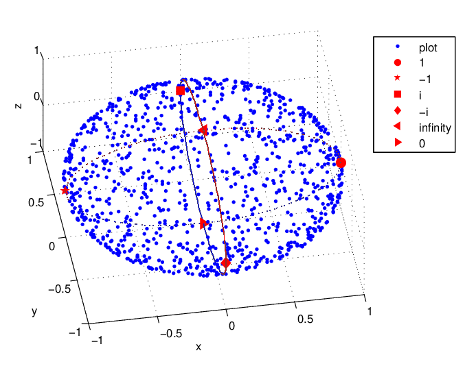
In the appendix, we give a picture which describes the distribution to random zeros of a given random polynomial. Let

p(z)=\sum^{50}_{i=1}c_{i}(C^{j}_{N})^{\frac{1}{2}}z^{i},

where ${\mathbf{E}}(c_{i})=0$ and ${\mathbf{E}}(|c_{i}|^{2})=1.$

References

[B] M.Baker, A lower bound for average values of amical green’s functions, 2006, NT/0507484
[BBP] B.Bergersen, D.Boal and P. Palffy-Muhoray , Equilibrium configurations of particles on a sphere: the case of logarithmic interaction, J. Phys. A: Math.Gen. 27 (1994) 2579-2586.
[BSZ] P. Bleher, B. Shiffman, and S. Zelditch, Steve Universality and scaling of correlations between zeros on complex manifolds. Invent. Math. 142 (2000), no. 2, 351–395.
[BSZ2] P. Bleher, B. Shiffman, and S. Zelditch, Universality and scaling of zeros on symplectic manifolds. Random matrix models and their applications, 31–69, Math. Sci. Res. Inst. Publ., 40, Cambridge Univ. Press, Cambridge, 2001.
[BSZ3] P. Bleher, B. Shiffman, and S. Zelditch, Poincare-Lelong Approach to Universality and Scaling of Correlations Between Zeros, Cimmunications in Mathematical Physics, (2000), 771-785.
[DKLR] Michael R. Douglas, Robert L. Karp, Sergio Lukic, Rene Reinbacher, Numerical Calabi-Yau metrics,hep-th/0612075
[H] L. Hörmander, The Analysis of Linear Partial Differential Operators III, Springer, 1980
[HS] D.P. Hardin, E.B. Saff, Discretizing manifolds via minimum energy points, Notices Amer. Math. Soc., Vol 51 (2004), 1186–1194.
[Hr] Hriljac P., Splitting fields of principal homogeneous spaces, Number Theory Seminar, Lect. Notes in Math. 1240, Springer-verlag, 1987, pp. 214-229
[KSh] A. Katanforoush and M. Shahshahani, Distributing points on the sphere. I. (English. English summary) Experiment. Math. 12 (2003), no. 2, 199–209.
[KS] A.B.J. Kuijlaars, E.B. Saff, Asymptotics for minimal discrete energy on the sphere, Trans. Amer. Math. Soc. 350 (2) (1998) 523–538.
[SS] M. Shub and S. Smale. ”Complexity of Bezout’s Problem III: Condition Number and Packing.” Jour. of Complexity 9 (1993), 4–14.
[SZ] B. Shiffman and S. Zelditch, Number variance of random zeros, math.CV/0512652.
[SZ1] B. Shiffman and S. Zelditch, Distribution of zeros of random polynomials and quantum chaotic sections of positive line bunldes. Commun. Math. Phys. 200. 661-683 (1999)
[SZ3] B. Shiffman and S. Zelditch, Number variance of random zeros on complex manifolds, math.CV/0608743

	$\displaystyle{\mathbf{E}}\mathcal{E}^{N}_{G_{g}}$	$\displaystyle=N\int_{M}\int_{0\leq\|u\|\leq b\sqrt{\log N}}[-\frac{1}{2\pi}\log(\frac{\sqrt{<B(z)u,u>}}{\sqrt{N}}+O(N^{-\frac{3}{2}}))][H(\frac{1}{2}\|u\|^{2})-1]\frac{\omega_{z}}{\pi}\otimes\frac{i}{2\pi}\partial\bar{\partial}\|u\|^{2}$
		$\displaystyle=\frac{1}{2\pi}N\log\sqrt{N}\int_{M}\frac{\omega_{z}}{\pi}\int_{0\leq\|u\|\leq b\sqrt{\log N}}[H(\frac{1}{2}\|u\|^{2})-1]\frac{i}{2\pi}\partial\bar{\partial}\|u\|^{2}$
		$\displaystyle\ \ \ -\frac{N}{2\pi}\int_{M}\int_{0\leq\|u\|\leq b\sqrt{\log N}}\log\sqrt{<B(z)u,u>}(H(\frac{1}{2}\|u\|^{2})-1)\frac{\omega_{z}}{\pi}\otimes\frac{i}{2\pi}\partial\bar{\partial}\|u\|^{2}+o(N)$
		$\displaystyle\sim\frac{1}{4\pi}N\log N\int_{0\leq\|u\|<\infty}[H(\frac{1}{2}\|u\|^{2})-1]\frac{i}{2\pi}\partial\bar{\partial}\|u\|^{2}$
		$\displaystyle\ \ \ -\frac{N}{2\pi}\int_{M}\int_{0\leq\|u\|<\infty}\log\sqrt{<B(z)u,u>}(H(\frac{1}{2}\|u\|^{2})-1)\frac{\omega_{z}}{\pi}\otimes\frac{i}{2\pi}\partial\bar{\partial}\|u\|^{2}+o(N)$
		$\displaystyle=I+II+o(N)$