Yerevan Physics Institute
After A.I. Alikhanyan
Lev Ananikyan
Spin Effects in Quantum Chromodynamics and
Recurrence Lattices with Multi-Site Exchanges
Thesis for acquiring the degree of candidate of physical-mathematical sciences
in division 01.04.02 (Theoretical Physics)
Scientific supervisor
Candidate of phys.-math. sciences
N. Ivanov
YEREVAN 2007
Chapter 1 Introduction and Motivation
It is widely accepted that the notion of spin was introduced by Uhlenbeck and Goudsmit to explain the data on the energy levels of alcaline atoms. The full story is, however, more intriguing and instructive. Pauli, in early 1925, decided that the electron has an extra ”classically undescribable” quantum number, and formulated his famous exclusive principle, according to which two electrons cannot be in the same state. This principle made it possible to avoid the difficulties in interpretation of atomic spectra and explain the counting of levels in weak and strong magnetic fields.
Pauli was not, however, willing to make the big jump that the electron has an intrinsic angular momentum . It was R.L. Kronig, who proposed this idea first. However, this idea was not well received by Pauli, as well as in Copenhagen where Kronig went visiting. There was also a problem about the spacing of the levels which gave doubts to Kronig himself. Then in the fall of 1925, Uhlenbeck and Goudsmit, in Leiden, proposed the same idea which they sent for publication to Naturwissenshaften [1]. After discussions with Lorentz, they tried to withdraw their paper, but it was too late (fortunately) and it was published! An excellent description of the history of spin and statistics can be found in Ref. [2].
Presently, spin is a powerful and elegant tool which plays a crucial role in both high energy physics and statistical mechanics. Spin is one of the most fundamental properties of elementary particles because it determines their symmetry behavior under space-time transformations.
High energy experiments with polarized beams or final-state spin effects provide often most deep insights into the properties of elementary particles and their interactions. For example, the world’s best measurements of the weak mixing angle, , have been provided by the SLD experiment at SLAC by using the left-right asymmetry in polarized scattering, as well as by the LEP results on the forward-backward asymmetry for -quark final states [3]. (For a review, see Refs. [4, 5].)
It is interesting to note that spin appeared in statistical mechanics also in 1925. The spin model in a magnetic field was first solved in one dimension by E. Ising [6] and for that reason it now bears his name. In 1944, Onsager [7] first computed the free energy for the two-dimensional Ising model. One of the most popular subjects of investigation in the modern statistical physics are critical phenomena in spin systems. Present status of our knowledge about the two- and three-dimensional equilibrium spin systems related to the Ising, Heisenberg and universality classes is discussed in Ref. [8]. Recent review on the spin glass models can be found in Refs. [9, 10].
It is well known that there is a close relation between the Quantum Field Theory (QFT) and Statistical Mechanics (SM). First, an external similarity there exist: the generating functional of a QFT in the Euclidean formulation looks the same as the partition function of corresponding statistical model. This similarity is, however, rather formal because both QFT and SM deal with an infinite number of degrees of freedom, and further definitions are always needed to remove corresponding divergences. A satisfactory understanding of the connection between QFT and SM was reached only when the ideas of the scaling observed in investigation of critical behavior of SM models were reconsidered in the general renormalization-group (RG) framework by Wilson [11, 12]. Using the field-theoretical methods, it was possible to explain the critical behavior of most of the systems and their universal features; for instance, why fluids and uniaxial antiferromagnets behave quantitatively in an identical way at the critical point.
On the other hand, the RG theory of critical phenomena provides the natural framework for defining quantum field theories at a nonperturbative level, i.e., beyond perturbation theory (see, e.g., Ref. [13]). In particular, the Euclidean lattice formulation of gauge theories proposed by Wilson [14, 15] provides a nonperturbative definition of Quantum Chromodynamics (QCD), the theory of strong interactions of elementary particles. QCD is obtained as the critical zero-temperature (zero-bare-coupling) limit of appropriate four-dimensional lattice models and may therefore be considered as a particular four-dimensional universality class (see, e.g., Refs. [13, 16, 17]). Wilson’s formulation represented a breakthrough in the study of QCD, because it lent itself to nonperturbative computations using statistical-mechanics techniques, for instance by means of Monte Carlo simulations (see, e.g., Ref. [18]).
In this thesis, we study some spin effects in QCD and recurrence lattices with multi-site exchanges. In the framework of QCD, we consider the azimuthal asymmetries in heavy flavor production in the lepton-nucleon deep inelastic scattering.
Investigation of the heavy flavor production plays a crucial role in QCD. This is because, for a sufficiently heavy quark, the cross sections are calculable as a perturbation series in the running coupling constant , evaluated at the quark mass. Thus, measurements of the heavy flavor production provide an excellent testing ground for perturbative sector of QCD. Moreover, the charm and bottom production is a good probe of the structure of the target hadron. In particular, the heavy quark photoproduction is a viable way to measure the gluon structure functions (both polarized and unpolarized), while the leptoproduction process is very sensitive at large Bjorken to the intrinsic charm content of the target.
In the framework of perturbative QCD (pQCD), the basic spin-averaged characteristics of heavy flavor hadro-, photo- and electroproduction are known exactly up to the next-to-leading order (NLO). During the last fifteen years, these NLO results have been widely used for a phenomenological description of available data. At the same time, the key question remains open: How to test the applicability of QCD at fixed order to heavy quark production? The problem is twofold. On the one hand, the NLO corrections are large; they increase the leading order (LO) predictions for both charm and bottom production cross sections by approximately a factor of two. For this reason, one could expect that higher-order corrections, as well as nonperturbative contributions, can be essential, especially for the -quark case. On the other hand, it is very difficult to compare pQCD predictions for spin-averaged cross sections with experimental data directly, without additional assumptions, because of a high sensitivity of the theoretical calculations to standard uncertainties in the input QCD parameters. The total uncertainties associated with the unknown values of the heavy quark mass, , the factorization and renormalization scales, and , and the parton distribution functions are so large that one can only estimate the order of magnitude of the pQCD predictions for total cross sections at fixed target energies [19, 20].
At not very high energies, the main reason for large NLO cross sections of heavy flavor production in [21, 22], [23], and [24, 25, 26, 27] collisions is the so-called threshold (or soft-gluon) enhancement. This strong logarithmic enhancement has universal nature in the perturbation theory since it originates from incomplete cancellation of the soft and collinear singularities between the loop and the bremsstrahlung contributions. Large leading and next-to-leading threshold logarithms can be resummed to all orders of perturbative expansion using the appropriate evolution equations [28, 29, 30]. Soft gluon resummation of the threshold Sudakov logarithms indicates that the higher-order contributions to heavy flavor production are also sizeable. (For a review see Refs. [31, 32, 33]).
Since production cross sections are not perturbatively stable, it is of special interest to study those (spin-dependent) observables that are well-defined in pQCD. A nontrivial example of such an observable was proposed in Refs. [34, 35, 36, 37] where the azimuthal asymmetry in heavy quark photo- and leptoproduction has been analyzed 11 1 The well-known examples are the shapes of differential cross sections of heavy flavor production which are sufficiently stable under radiative corrections.. In particular, the Born level results have been considered [34, 36] and the NLO soft-gluon corrections to the basic mechanism, photon-gluon fusion (GF), have been calculated [35, 36]. It was shown that, contrary to the production cross sections, the asymmetry in heavy flavor photo- and leptoproduction is quantitatively well defined in pQCD: the contribution of the dominant GF mechanism to the asymmetry is stable, both parametrically and perturbatively. This fact provides the motivation for investigation of the photon-(heavy) quark scattering (QS) contribution to the -dependent lepton-hadron deep inelastic scattering (DIS).
In the present thesis, we calculate the azimuthal dependence of the next-to-leading order (NLO) heavy-flavor-initiated contributions to DIS. To our knowledge, pQCD predictions for the -dependent cross sections in the case of arbitrary values of the heavy quark mass and are not available in the literature. Moreover, there is a confusion among the existing results for azimuth-independent cross sections.
The NLO corrections to the -independent lepton-quark DIS have been calculated (for the first time) a long time ago in Ref. [38], and have been re-calculated recently in [39]. The authors of Ref. [39] conclude that there are errors in the NLO expression for given in Ref. [38] 22 2 For more details see PhD thesis [40], pp. 158-160.. We disagree with this conclusion. It will be shown below that a correct interpretation of the notations for the production cross sections used in [38] leads to a complete agreement between the results presented in Refs. [38], [39] and present thesis.
As to the -dependent cross sections, our main result can be formulated as follows. Contrary to the basic GF component, the QS mechanism is practically -independent. This is due to the fact that the QS contribution to the asymmetry is absent (for the kinematic reason) at LO and is negligibly small (of the order of ) at NLO. This fact indicates that the azimuthal distributions in charm leptoproduction could be a good probe of the charm density in the proton.
Then we investigate the possibility of measuring the nonperturbative intrinsic charm (IC) 33 3 The notion of the IC content of the proton has been introduced over 25 years ago in Refs. [41, 42]. This nonperturbative five-quark component, , can be generated by fluctuations inside the proton. using the asymmetry. Our NLO analysis of the hadron level predictions shows that the contributions of both GF and IC components to the asymmetry in charm leptoproduction are quantitatively well defined: they are stable, both parametrically and perturbatively, and insensitive (at ) to the gluon transverse motion in the proton. At large Bjorken , the asymmetry could be a sensitive probe of the intrinsic charm content of the proton.
We have also considered the contribution to azimuthal distributions of the perturbative charm density within the variable flavor number scheme (VFNS) [43, 44] 44 4 The VFNS is an approach alternative to the traditional fixed flavor number scheme (FFNS) where only light degrees of freedom ( and ) are considered as active. Within the VFNS, potentially large mass logarithms are resummed through the all orders into a heavy quark density which evolves with according to the standard evolution equation.. Main result of our analysis is that the charm densities of the recent CTEQ [45] and MRST [46] sets of parton distributions have a dramatic impact on the asymmetry in the whole region of and, for this reason, can easily be measured.
Concerning the experimental aspects, azimuthal asymmetries in charm leptoproduction can, in principle, be measured in the COMPASS experiment at CERN, as well as in future studies at the proposed eRHIC [47, 48] and LHeC [49] colliders at BNL and CERN, correspondingly.
Another topic of our thesis are critical phenomena in spin systems defined on the recurrence lattices with multi-site exchanges. It is well established that the thermodynamic properties of a physical system can be derived from a knowledge of the partition function. Since the discovery of statistical mechanics, it has been a central theme to understand the mechanism how the analytic partition function for a finite-size system acquires a singularity in the thermodynamic limit when the system undergoes a phase transition. The answer to this question was given in by Lee and Yang in their seminal papers [50, 51]. It was shown that phase transitions occur in the equilibrium systems in which the continuous distribution of zeros of the partition function intersects the real axis in the thermodynamic limit. For anti-ferromagnetic Potts models, by contrast, there are some tantalizing conjectures concerning the critical loci, but many aspects still remain obscure [52, 53, 54]. Recently, the Yang-Lee formalism has also been applied for investigation of nonequilibrium phase transitions [55].
Presently, the investigation of the partition function zeros is a powerful tool for studying phase transition and critical phenomena. Particularly, much attention is being attached to the study of zeros of partition function of helix-coil transition of biological macromolecules [56, 57, 58, 59].
In this thesis, we investigate helix-coil phase transition for polypeptides and proteins in thermodynamic limit on recursive zigzag ladder with three-spin interaction. We use recursive lattices because for the models formulated on them the exact recurrence relations for branches of the partition function can be derived. For classical hydrogen bond (), we have got the Yang-Lee zeros corresponding to helix-coil phase transitions for polypeptides and proteins in thermodynamic limit. We also take into account a non-classical helix-stabilizing term describing a hydrogen bond of the type . For this case we obtain folding and quasi unfolding of the order parameter (degree of helicity ). Applying multi-dimensional mapping on zigzag ladder, we got Arnold tongues for non-classical helix-coil phase transition for neutral points of mapping 55 5 Neutral points are defined by condition that eigenvalues of the mapping Jacobian, , lie on the unit circle, ..
There are two types of modulated phases: commensurate and incommensurate ones. For commensurate phases, when , the so-called Arnold tongues there exist. Typically, for multi-dimensional maps, the border of such regions (Arnold tongues [60]) splits into two branches in the parameter space.
Our main result is that we get two qualitatively different behaviors for the degree of helicity that depend on input parameters. The first regime presents a low-temperature helix structure which melts at higher temperatures. We observe that the presence of a non-classical () interaction sensibly enhances the melting temperature, and the transition is smooth. In second case, the presence of non-classical interaction leads to a remarkably different low-temperature behavior. In this regime, an quasi unfolding transition takes place for as well, like to cold denaturation [61]. We point out that our results are meaningful for long chains since, for such chains, a thermodynamic limit is involved. Note that unfolding of biopolymer has also been observed in phenomenological model [62], Monte Carlo simulation [63], Bethe approximation [64], and for a short chain in Distance Constraint Model [65].
In this thesis, we also investigate magnetic properties of the 3He. Investigation of magnetic phenomena and magnetic properties of materials has a long history [66]. The theory of magnetism and related problems composes a fast and rather advanced field of research in the modern theory of condensed matter physics intimately linked to many other fields of physics, mathematics, biophysics, chemistry and materials science. These investigations have a wide application in various fields of electronics, computer techniques e.t.c. The unexpected discovery of cooper-oxide high- superconductors in 1986 [67] not only aroused hopes that one day we will have at our disposal materials which exhibit superconductivity at room temperature, but also opened a new stage in the studies of magnetic phenomena. This is because there is a strict evidence that two-dimensional anti-ferromagnetism is one of the key components of high-temperature superconductivity. One of the most remarkable achievements in this field is the progress in the studies of magnetism in solid 3He.
Solid and fluid 3He films absorbed on the surface of graphite have attracted extensive attention since (at low temperatures and high pressures, due to the light mass of helium atoms) it is a typical example of a two-dimensional frustrated quantum-spin system [68, 69]. The nuclei of 3He are fermions with spin 1/2. It’s reasonable to assume that solid 3He is a system of localized identical fermions. The microscopic theory of magnetism for such systems is based on the concept of the permutation of particles. In the films under consideration, the nuclei of 3He form a system of quantum 1/2 spins on a triangular lattice. We know experimentally that the three-particle interactions dominate in this system. Transition from ferromagnetic behavior to antiferromagnetic one takes place when the coverage density of 3He atoms decreases. The explanation is suggested in terms of multiplespin exchanges MSE. In a dense clode-packed solid, ferromagnetic three-spin exchange is dominant [70]. At lower densities, ferromagnetic three-and-five spin exchanges compete with antiferromagnetic four-and-six spin exchanges and lead to a frustrated antiferromagnetic system. The MSE produce frustration by themselves and a strong competition between odd and evenparticle exchanges is also responsible for the frustration [71]. For description of solid 3He films, one can use the dynamical system approach with MSE model that leads to appearance of various ordered phases and magnetization plateaus and one period doubling [72, 73]. The study of the above mentioned magnetization plateau is one of the main directions of present-day activity in the field of non-trivial quantum effects in condensed matter physics. Despite the purely quantum origin of this phenomenon, it was shown recently that magnetization plateau can appear in the Ising spin systems as well exhibiting in some cases fully qualitative correspondence with its Heisenberg counterpart [74, 75, 76, 77].
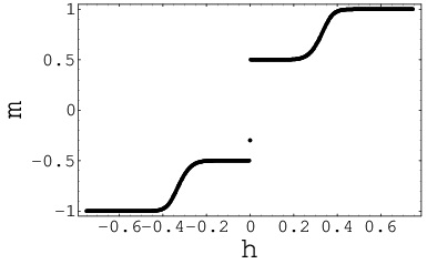
Using the dynamical system approach with MSE on the recurrent lattices (square, Husimi, hexagon), we obtain magnetization curves with plateaus (at and ) and one period doubling.
The next issue of our investigation is the so-called face-cubic model. We have considered a spin model with cubic symmetry defined on the Bethe lattice and containing both linear and quadratic spin-spin interactions. An expression for the free energy per spin in the thermodynamic limit was obtained. We have applied the methods of the dynamical systems theory or, more precisely, the theory of discrete mappings. In this technique, one exploits the self-similarity of the Bethe lattice and establishes a connection between the thermodynamic quantities defined for the lattices with different number of sites.
We have identified the different thermodynamic phases of the system (disordered, partially ordered and completely ordered) in the ferromagnetic case (, ) with different types of the fixed points of recurrent relation. Then we have obtained the phase diagrams of the model which are found to be different for and . The case of contains three tricritical points while only one tricritical and one triple points there exist at .
Our results on the critical phenomena in spin systems defined on recurrence lattices with multi-site exchanges are published in Refs. [78, 79, 80, 81, 82, 83]. Our studies of the spin effects in QCD are presented in Refs. [84, 85].
The thesis is organized as follows. In Chapter 2, the multi-dimensional mapping is used for non-classical helix-coil phase transition of anti-ferromagnetic Potts model for biopolymer formulated on the recursive zigzag ladder. Two qualitatively different behaviors for the degree of helicity are obtained.
In Chapter 1, three types of the recurrent lattices with MSE are considered as approximation to solid 3He films. Using methods of the dynamical systems theory, we’ve got magnetization plateaus, bifurcation points, one period doubling behavior and modulated phases at sufficiently high temperatures.
In Chapter 4, we derive the system of recurrent relations for the face-cubic model on the Bethe lattice. We identify different types of the fixed points of the system of recurrent relations with different physical phases.
In Chapter 5, we analyze the QS and GF parton level predictions for the -dependent charm leptoproduction in the single-particle inclusive kinematics. Hadron level predictions for azimuthal asymmetry are obtained. We consider the IC contributions to the asymmetry within the FFNS and VFNS in a wide region of and .
Main observations and conclusions of this thesis are discussed in Conclusion.
Chapter 2 Advantage of Recursive Lattices 11 1 The results considered in this chapter are published in Refs. [78, 79].
The advantage of recursive lattices is that for the models formulated on them the exact recurrence relations for branches of the partition function can be derived. Let us consider the recursive lattices which are connected through the sites. As the first example of recursive lattice is an usual chain. One can receive the exact recursion relation for the partition function for Ising model. We divide a chain on two equal parts. The partition function can be written as follows:
| (2.1) |
where is the center of the chain and is the contribution of each chain branch. can be expressed trough , that is, the contribution of the same branch containing n-1 generations starting from the site belonging to the first generation:
| (2.2) |
where takes values 1, J is interaction constant and is the external magnetic field. We introduce the following variable
| (2.3) |
where we denote by if the spin takes the value +1 and by if the spin takes the value -1. For we can then obtain the recursion relation:
| (2.4) |
is a ratio of two polynomials. We obtain one dimensional dynamic rational mapping. We can get the magnetization of a central site through .
Another example of recursive lattice is the Bethe one. Let us regard the Potts model on this lattice with coordination number. The Hamiltonian can be written as:
| (2.5) |
where for and 0 otherwise, takes the values 1,2,…Q, the first sum is over the nearest-neighbor sites, and the second sum is simply over all sites on the lattice. We use the notation K=J/kT and h=H/kT. Cutting apart the Bette recursive lattice at the central point we get identical branches. As usual we can receive one dimensional dynamic rational mapping for partition function. The same ideas can be used as for the recursive chain. Denoting the contribution of each lattice branch one can receive the recursive dynamic relation. Introducing the notation
| (2.6) |
one can obtain the Potts-Bethe map
| (2.7) |
The magnetization of the central site for the Bethe lattice can be written as
| (2.8) |
The situation changes drastically for with antiferromagnetic interactions. The plot of the M (magnetization) versus h (external magnetic field) has a bifurcation point and chaotic behavior at low temperatures [86].
An other example is Husimi lattice. It can be regarded as recursive lattice. The three-site antiferromagnetic Ising model on Husimi lattice is investigated in an external magnetic field using the dynamic system approach. Making the same procedure for Husimi recursive lattice one can obtain one dimensional rational recursive relation for partition function. The full bifurcation diagram, including chaos, of the magnetization was exhibited. It is shown that this system displays in the chaotic region a phase transition at a positive ”temperatures” whereas in a class of maps close to , the phase transitions occure at negative ”temperatures”. The Frobenius-Peron recursion equation was numerically solved and the density of the invariant measure was obtained [87].
The ladders [88, 89, 90] also can be regarded as a recursive lattice. They are connected through the bonds and have multi dimensional rational mapping for partition function. A zigzag ladder with axial next-nearest-neighbor Ising model has attracted many investigators on account of the fact that it is a particularly simple model exhibiting quasi specially modulated phases that can be either commensurate or incommensurate with the underlying lattice [91]. Using the dynamic approach one can receive three dimensional rational mapping for partition function.
2.1 Arnold Tongues in Ising and Potts Models
Let us regard the anti-ferromagnetic Ising and Potts models on the recursive Bethe lattice connected through sites. For Ising model the partition function can be written as:
| (2.9) |
where is the central spin, - the contribution of each lattice branch, - magnetic field and - coordination number[92]. is obviously expressed through :
| (2.10) |
for and interaction between the spins is constant . Introducing the notation
| (2.11) |
the recursion relation (2.10) can be rewritten in the form
| (2.12) |
As is known, if the derivative of is equal to we have a bifurcation point, corresponding to the second order phase transition for anti-ferromagnetic model. We defined and after a simple calculation we have got the following system of equations:
| (2.13) |
Eliminating we obtain the following equation:
| (2.14) |
Solving this equation we get:
| (2.15) |
This equation define Arnold tongues between paramagnetic and modulated phases with winding number .

The Arnold tongue begins at the temperature of , when the external magnetic field , and ends () at (see figure 2.1).

The same procedure we can perform for anti-ferromagnetic Potts model on recursive Bethe lattice with Hamiltonian
| (2.16) |
where takes the values . Introducing the notation
| (2.17) |
where is the branch of partition function with central spin and is the branch of partition function with central spin . For the coordination number of the Bethe lattice we obtain following system of equations
| (2.18) |
here again the derivative of is equal to which corresponds to the second order phase transition of anti-ferromagnetic model and where . The Arnold tongue begins at , when external magnetic field , and ends () at and (see figure 2.2).
2.2 Multi-dimensional Mapping for the Biological Macromolecules
The structure of a protein is completely encoded in the amino-acid sequence [93]. Understanding of the folding and unfolding processes of proteins (hetero-polymers) and polypeptides (homo-polymers) is one of the current challenges in molecular biophysics. A lot of effort has been devoted to clear up the mystery of protein or polypeptide folding nature by using lattice models [94]. These simple lattice models single out the formation of a helix structure in protein as the basic mechanism to be understood. Thermodynamics of homo and hetero-polymers folding has been investigated in this perspective by introducing a variety of different lattices: chains [95, 96, 97], square lattices [98, 99], and cubic ones [100, 101]. Off-lattice models have been discussed by Irback et al. and Klimov and Thirumalai [102, 103]. Chaotic behavior in off-lattice models of hetero-polymers (proteins) and folding and unfolding have been analyzed in two-dimensional systems by means of Monte Carlo simulations [104]. The theory of finite-size scaling of helix-coil transition was studied by Okamoto and Hansmann [56, 57, 58, 59] by multi-canonical simulation. They have chosen three types of polypeptides with aliphatic neutral amino acids (alanine, valine, and glycine). It was shown that -helix formation in short peptide systems agrees with experimental results [105]. But proteins are composed of different types of monomers. Hydrophobic monomers, such as leucine or proline, try to hide their surfaces from the solvent. The simplest protein theoretical model divides the amino acids into two categories: hydrophobic (H) and polar (P) surrounded by the solvent [106, 107]. Kamtekar et al. [108] made experiments with a variety of hydrophobic (H) and polar (P) amino acids in hetero-polymers and showed that a simple code of polar (P) and nonpolar hydrophobic (H) residues arranged in an appropriate order could drive polypeptide chains to collapse into globular -helical folds.By using a simple HP lattice model [109, 110] a theory explained the experimental phenomenon of cold denaturation (unfolding) on real proteins [61]. The study of relaxation processes in biopolymer is of particular significance since the functional abilities of thes molecules are related to the dynamical properties [111].
We point out that different theoretical models were proposed to study both unfolding and folding of proteins [62].
From a statistical mechanics perspective different approaches can be attempted to investigate the nature of the helix-coil phase transition: from the analysis of Yang-Lee zeroes [50, 51], to multicanonical Monte Carlo simulation for finite samples [56, 57, 58, 59, 98, 99, 100, 104, 109, 110].
In this thesis we study in thermodynamic limit a model for the helix structure of proteins and polypeptides, where we take into account both the classical hydrogen bond [112] between three -carbons by using and H-bond connection, and the non-classical H-bonds [113] in every . The classical ( helix) H-bond is formed in the following way: three neighboring angle pairs [ and ] form a H-bond when rotations are such that the distance between H and O becomes less than 2 Å (fig.1). The hydrogen bond is a unique phenomenon in structural chemistry and biology. Its functional importance stems from both thermodynamic and kinetic reasons. In supermolecular chemistry, the hydrogen bound is able to control and direct the structures of molecular assemblies because it is sufficiently strong and sufficiently directional. The subject of hydrogen bonding is of major interest and remains relevant with each new phase in the kaleidoscope of chemical and biological research (see references in [114]). Non-classical bonds have been recognized to play an important role in biological macromolecules (see [115]), and they were for instance observed between water and amino acids alanine [] [116] or between two helices of collagen [117].
Traditionally, the transition from random coiled conformation to the helical state in DNA, RNA or proteins are described in the framework of Zimm-Bragg [118] type Ising model. But this type of one-dimensional model cannot account for non-trivial topology of hydrogen bonds [112].


We show the backbone chain of the polypeptide molecule in fig. 2.3. R (amino acid residue) denotes the side chain. Because of the planar structure of the amide group, almost the whole conformational flexibility of the polypeptide backbone chain is determined by the rotation angles around the single bonds and which are usually denoted as and respectively.
We now formulate our model: first of all the angle pairs are discretized [119], the possible values are labeled by a discrete variable .When three successive rotation pairs (spins) are zero (), an H-bond appears which leads to some energy gain. When one of three neighboring spins is not zero() an interaction with solvent is taken into account. This leads to a three-site interaction Potts model [120] on a zigzag ladder (see fig. 2.4) The Hamiltonian of the system is written as
| (2.19) | |||
where is the energy of hydrogen bond, is the energy of protein-solvent hydrogen bond, denotes the Potts variable at the site and takes the values , is the energy of non-classical H-bond, and label each triangle in Fig. 2.4.
The model we thus introduced is indeed quite a simplified one, but it allows to discuss how non-classical bonds compete with classical hydrogen interaction in an idealized setting. We will take advantage of the recursive nature of the zigzag ladder: this makes it possible to derive exact recursion relations for branches of the partition functions, and in this way statistical properties in the thermodynamic limit may be investigated by dynamical systems techniques [78]. In their simplest realization recursive relations yield one dimensional mappings [92, 73].
By cutting the zigzag ladder in the central triangle () one gets the partition function associated to the hamiltonian (2.19)
| (2.20) |
where
| (2.21) |
T is temperature (room temperature is ), are spins of central triangle, and are the parts of partition function corresponding to two branches, is generation of recursive lattice (see Fig.2.4). By introducing the following notation
| (2.22) |
and
| (2.23) |
(2.20) can be rewritten as:
| (2.24) | |||
By applying the ”cutting” procedure to an th generation branch one can derive the recurrence relations for ,
| (2.25) | |||
If we notice that , and introduce the notation
| (2.26) |
we can obtain a two-dimensional mapping from (2.25),
| (2.27) | |||
2.3 Helicity and Arnold Tongues for the Macromolecules
The (dimensionless) order parameter or helicity defined as
| (2.28) |
where (when recursion relations admit a stable fixed point the order parameter is independent of the triangle we consider). Since our procedure implicitly involves a thermodynamical limit, its biological significance is motivated by the existence of long chains of proteins, like collagen, that may exist in the form of three intertwined peptide chains, each containing a thousand of amino acids (we also remark that the importance of non-classical H bonds in collagen has been pointed out in [117]).
Thus our task is that of investigating the asymptotic behavior of recursion relations (2.27), this allow to characterize the macroscopic order parameter as a function of the physical parameters T, (energy of classical H bond), (energy of protein-solvent H bond) and (energy of non-classical H bond).
We observe that in the whole range of the parameters triplet ( the recursion relations (2.27) admit a single (real) fixed point (). An investigation of the Jacobian matrix of the transformation at () moreover indicates that such a fixed point is always stable: thus we do not get any phase diagram marked by the stability border for the fixed point like in mean field Ising models with competing interactions on hierarchical lattices [121]. We also point out that we did not observe in our tests any other dynamically relevant attracting structure: under iteration of (2.27) generic initial conditions collapse to the stable fixed point. (We mention that for physical values of microscopic parameters there exist complex fixed points () at which the absolute value of eigenvalue of Jacobian equals to one. In this case the order parameter () would be complex too).

Once () is determined, the degree of helicity (2.28) can be computed. Our main result is that we get two possible qualitatively different behaviors. The first regime presents a low-temperature helix structure, which melts at higher temperatures (see fig.2.5), a qualitative feature that may be observed if the non classical interaction is absent. By looking at two of the curves in fig.2.5 we observe that the presence of a non-classical () interaction sensibly enhances the melting temperature, and that, coherently with the dynamical analysis of recursion relation, the transition is smooth. For other parameter values, the presence of non-classical interaction leads to a remarkably different low temperature behavior, with an quasi unfolding transition also for , akin to cold denaturation [61], see fig.2.6. Real unfolding behavior is when order parameter’s peak is near one. In fig.2.6 for parameters: and we have a strange situation. At low temperature we have a coil. The protein changes conformation upon heating. Some of and in average are near and they form H-bond. In these parameters the degree of helicity (order parameter) becomes larger. We call that quasi helix. At higher temperature the protein becomes coil again.

Using the theory of dynamical systems for two-dimensional mapping, we have obtained the separating line, which divides the coil (paramagnetic, disordered) phase from helix (modulated, ordered) one (see figure 2.7).Two example of Arnold tongues for non-classical helix-stabilizing interaction with for and are shown on figures 2.8, 2.9.


We point out that our result are meaningful for long chains, since a thermodynamic limit in the statistical model is involved. We notice however that unfolding of biopolymer has been observed in phenomenological model [62], Monte Carlo simulation [63], Bethe approximation [64], and for a short chain in Distance Constraint Model [65].
2.4 Yang-Lee Zeroes for the Biological Macromolecules
When we take into account only classical hydrogen bound the Hamiltonian of the system is written as
| (2.29) |
We obtain again the two dimensional rational mapping relation for and
| (2.30) |
where
| (2.31) |
In case of multi-dimensional rational mapping the fixed point is attracting when the eigenvalues of Jacobian , repelling, when , and neutral, when . So the system undergoes a phase transition when
| (2.32) |
After eliminating and from (2.4) and (2.32) we obtain the following equation for the partition function zeros
| (2.33) |
where
| (2.34) |
One can solve (2.33) for and find the Yang- Lee zeros of partition function with different parameters , and like in Refs.[122]. These parameters are different for each polypeptides and proteins.

After making discrete values of and comparing with Ramachardan and Shceraga[119] we confirm that the circle in classical helix-coil transition does not cut the real axis. So we have not a real phase transition in polypeptides (proteins). According to phenomenological theory of Zimm-Bragg or Lifson-Roig there is only pseudo phase transition in 2-site (Ising) model. Our results describe the microscopic theory of helix-coil transition of polypeptides or proteins with non-trivial topology of hydrogen bonds and find Yang-Lee zeros of pseudo phase transition. Yang-Lee zeroes of helix-coil transition for polyalanine, polyvaline and polyglysine was regarded [56]. The authors made Monte Carlo simulation technique and considered polypeptide chain up to monomers and determine the (pseudo) critical temperatures of the helix-coli transition in all-atom model of polypeptides.
Chapter 3 Fluid and Solid 3He 11 1 The results considered in this chapter are published in Refs. [80, 82, 83].
As mentioned in introduction, fluid and solid 3He films absorbed on the surface of graphite have attracted extensive attention, since it is a typical example of a two-dimensional frustrated quantum-spin system [68, 69]. The first and second layer of the nuclei of 3He forms a system of quantum one-half spins on a triangular lattice. The third layer forms a Kagome one [123]. Many experimental [124] and theoretical [125] studies suggest that the exchange of more than two particles are dominated in these systems. For such systems a change from ferromagnetic behavior to anti-ferromagnetic takes place. Spin ladder anti-ferromagnets have been attracting extensive interest because they have a spin gap. A special type of frustration due to cyclic exchange interactions was recently found to be important in the spin ladder material LaxCa14-xCu24O41 [88]. It is experimentally also known that a many-body exchange interaction cannot be neglected especially in 3He on graphite [126].
Last decade the investigation of magnetization plateaus in a strong magnetic field has taken on special significance. The magnetization plateaus are famous for the fact that they are an example of essentially macroscopic quantum phenomenon. For the first time, Hida has theoretically predicted an appearance of the magnetization plateau for the ferromagnetic-ferromagnetic-antiferromagnetic Heisenberg chain of 3CuCl2 dioxane compound, which consist of the antiferromagnetic coupled ferromagnetic trimers [127]. The values of magnetization at which the plateaus appear are quantized to fraction values of the saturation magnetization. The theoretical explanation of this fact was been given in 1997 by Oshikawa, Yamanaka and Affleck [128]. These magnetization plateaus were observed as a simple origin in the Ising limit [129]. Geometric frustrated quantum magnets are a class of magnetic materials with various unusual properties at low temperature and high pressure. Due to strong frustration and quantum effects, these materials may be in principle considered as a source of new strongly correlated physics. The most of studied geometric frustrated quantum magnets are the Kagome and pyrochlore lattices of antiferromagnetic coupled nearest neighbor spins. As mentioned above, the third layer of the nuclei of 3He forms a Kagome lattice. Usually, the antiferromagnetic Kagome nets are investigated using numerical simulations [130]. We propose a dynamic approach based on exact recursive relations for partition functions. Our method makes possible to research magnetization plateaus, bifurcation points and period doubling in anti-ferromagnetic case at low temperatures and high pressures.
3.1 Ising Model Approach to the Solid 3He System on the Square Recursive Lattice
The most general expression for the Hamiltonian with multi spin-exchanges on a triangular lattice is
| (3.1) |
The term describes the phonon contribution and is not essential. responses for two-, three-, and four exchange interactions. term is responsible for magnetism in solid 3He and is given by Zeeman Hamiltonian
| (3.2) |
where is gyromagnetic ratio of the 3He nucleus.
One can write down exchange Hamiltonian for the first and second layers of planar solid 3He in the following way:
| (3.3) |
where sum in first term is going over all pairs of particles, in second term over all triangles and in third term over all rectangles consisting of two triangles.
The expression of a pair transposition operator has been given by Dirac,
| (3.4) |
where is the Pauli matrix, acting on the spin at the position number . The operator in general works in entirely different way, but in case of the pair transplonation operators are equal , that we can’t write in case of .
For we have
| (3.5) |
and
| (3.6) |
Using the identity
| (3.7) |
we can write the former expression as
| (3.8) |
and
| (3.9) |
hence
| (3.10) |
The four-spin permutation operators can be written as:
| (3.11) |
| (3.12) |
where the sum is taken over six distinct pairs () among the four particles (ijkl), and
| (3.13) |
So, in terms of Pauli matrices, we have:
| (3.14) | |||||
For the first and second solid layers, we consider a recursive lattice, instead of the periodic triangular one. This lattice is given in Fig.3.1.
We can attach to each site of the central plaquette a new one. Carrying out this procedure successively for each new shell, we can obtain a recursive lattice which actually is Bethe-type lattice of square plaquettes with additional inner links . It is evident that, for each plaquette, the coordination numbers of its sites are 6 or 5. Introducing the following parameters,
| (3.15) | |||||
| (3.16) | |||||
| (3.17) | |||||
| (3.18) |
the Hamiltonian can be rewritten as:
| (3.19) | |||||
If we use the multisite interaction Ising model, Eq. (3.19) takes the following form:
| (3.20) | |||||
where takes values .
The partition function takes the form [80]:
| (3.21) | |||||
where are spins of central plaquette, denotes contribution of branch at a-th site of central plaquette and is the number of generations ( case corresponds to the thermodynamic limit and neglecting the surface effects). For both values () of , one can easily calculate:
| (3.22) | |||||
| (3.23) | |||||
where the following notations has been introduced:
| (3.24) |
3.2 Magnetic Properties of the Antiferromagnetic Model on the Square Lattice
The recursion relation (3.25) plays the central role in our further investigations. Because it provides all the thermodynamic properties of the system. In particular, analogously, recursion relation for the magnetization per site,
| (3.30) |
can be derived.
| (a) | (b) |
|---|---|
 |
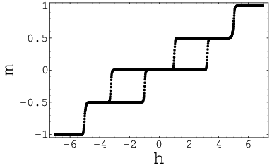 |
Let us describe the magnetic behavior of our model in a strong magnetic field. For the 3He films recent experimental measurements predict the following relations between the exchange energies on the regular triangular lattice:
| (3.31) |
The main features of the resulting magnetic behavior of the system under consideration are caused by the interplay between ferromagnetic () and antiferromagnetic ( and ) interactions. Also we use the well-known relations between exchange parameters ), which have been estimated from susceptibility and specific-heat data in the low density region [70]:
| (3.32) |
3.3 Recursive Approximation to Kagome Lattice
Since the density ratio of the third layer of is less then the first and second ones, it can use a Kagome lattice[123, 130]. For using the dynamic system approach it is necessary to approximate the Kagome lattice by recursive one. We use the Husimi lattice with two triangles coming out from one site (see Fig.3.3).

In this case
| (3.33) |
and
| (3.34) |
where is the gyromagnetic ratio of the 3He nucleus. The two-,and three-spin exchanges are given by Eq.(3.4) and Eq.(3.10). We have done further approximation passing to classical Ising model as in the solid case [80].
The partition function for recursive lattice is written in the form:
| (3.35) |
Here takes the values , is the central spin and denotes the contribution of each branch of the partition function.
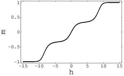
Introducing, as in previous section, , and one can receive the exact one dimensional rational mapping for partition function
| (3.36) |
where and .
| (a) | (b) |
 |
 |
| (c) | (d) |
 |
 |
The magnetization Eq.(3.30) as a function of , temperature and external magnetic field can be written as:
| (3.37) |
As an example, we take the temperature and obtain the figures of m(magnetization) versus h(external magnetic field)(see Fig.(3.4)). We take since the antiferromagnetic pair exchange interaction may be larger than the ferromagnetic three-spin interaction on a Kagome-type lattice.
3.4 Hexagonal Recursive Lattice as an Approximation of the Triangular One
One can write down the exchange Hamiltonian for planar solid He in the following way:
| (3.38) | |||||
where the sum in the first term is going over all pairs of particles, in the second term over all triangles and so on see figure 3.5.
Using the same technique as in Sec.3.1 we can derive expressions for fith and sixth exchange ineractions
| (3.39) |
| (3.40) |
where is
| (3.41) | |||||

Now let us consider the recursive lattices which are connected through the sites for getting onedimensional rational mapping which is close to triangular lattice. The central hexagon is approached to the triangular lattice by connection of center to vertices of hexagon, so we get six triangles in the central hexagon. The recursive lattice is constructed by adding next shells branches of hexagons on vertices of previous one see figure 3.5. Next shells are constructed in the same way. For hexagonal recursive lattice we obtain the exact recursive relations for partition function. It’s important to mention that this recursive relation is dynamic.
By now we considered Heisenberg model for description of our recursive lattice. We can assume that in the strong external magnetic field all atom’ spins will be directed mostly by certain z axis. So it will be possible to calculate the eigen-values of spinoperators. One may consider the variables as classical vectors as well as Pauli matrices. If we use the multisite interaction Ising model, we can take +1 and -1 instead of . In the rest of the paper all constance will be taken in temperature’s scaling .
When the lattice cut apart from the central hexagon, it separates into six identical branches. So we can first realize a summation over all spin configurations on each branch, getting the same result every time, and then the sum over spins of the central hexagon. Here follows, that we can represent the partition function as
| (3.42) | |||
| (3.43) |
from which the expression takes the form
| (3.44) | |||||
where
| (3.45) | |||||
We can obtain the recurrent relation for the variable :
| (3.46) | |||||
This recurrent relation plays a crucial role in our further investigations, because it’s getting possible obtain all thermodynamic quantities of the considered system.
3.5 Magnetic Properties of the Antiferromagnetic Model on the Hexagonal Recursive Lattice
Using the technique of dynamic system theory, applied to onedimensional rational mapping, we can get magnetization relations per site. As mentioned above for an homogeneous lattice the magnetization function is given by the formula
| (3.47) |
where is the spin on an arbitrary site. In our case, the lattice is homogeneous, so on central hexagon we divided the tree of hexagons on six branches.
We could obtain the magnetization value of sublattice composed by hexagon central vertices.
| (3.48) |
and for magnetization sublattice composed by corner verticies.
| (3.49) |
So from this expressions finally we could get
| (3.50) | |||||
and
| (3.51) | |||||
Having these dynamical expressions one can draw the plots of magnetization vs. external magnetic field for sublattices in various temperatures. To do that one should fix the value of the dimensionless magnetic field for a given temperatures and exchange parameters and implement the simple iteration from the recursion relation for , beginning with some initial . For achieving to the thermodynamical limit we have to apply infinite amount of iterations .
From experimental measurements and theoretical calculations we could conclude that the relations between the exchange energies on the regular triangular lattice are[68][70][69]:
| (3.52) |
It’s important to mention that the values of pure are not observable in the experiment measurements, because each n-spin exchanges makes also a contribution to a few -spin exchanges, and thus there are some effective exchanges parameters, which are certain contributions of such as and and can be directly obtained from experiments [68, 69, 70, 128].
The exchange parameters depend on the particle density and on the type of the lattice, particularly on its coordination number and dimensionality. For instance, it was found that for 2D triangular lattice at high densities the exchange is dominant, mainly due to the three-spin exchange, but the ratio increases rapidly with the lowering of the particle density, and below other exchanges become important also. The magnetic properties of the system ferromagnetic or antiferromagnetic depend on which exchange interactions are dominant at the present value of the particle density.
From the arguments stated above one can conclude that there is a large freedom in the choice of concrete values of the exchange parameters , , , and . Moreover, it is quite difficult to identify our model, having so many assumptions, with some concrete value of particle density.
The simplest case of pure ferromagnetic behavior is presented on figure 3.6. Figure 3.6a represents the magnetization for the central vertex of hexagon recursive lattice with temperature 0.1, figure 3.6b the magnetization for the corner vertex lattice with temperature and figure 3.6c the average magnetization for the lattice with temperature . At relatively high temperatures the magnetization curve has a smooth monotone form of Langevin type with a rather large value of the saturation field. Decreasing the temperature, the curve becomes more steep and the value of the saturation field decreases. Further decreasing the temperature leads to the magnetization diagram. We can see smoothly increasing curves, which are expected and corresponding to only ferromagnetic interactions.
The physical case with ferromagnetic and antiferromagnetic interactions for enough high temperature is represented on figure 3.7. On plots we can see the paramagnetic limit as expected in high temperatures.


There is represented the depends between external magnetic field and magnetization on figure 3.8 a is the magnetization for the central vertex lattice with temperature , (b) is the magnetization for the corner vertex lattice with temperature , (c) is the average magnetization for the lattice with temperature for physical case with , , , , . The hatch line represents the magnetization value with . On figure 3.8 we can see bifurcation points in high magnetic fields. This fact is making clear the advantage of represented model in high external magnetic field.There is a one period doubling behavior between bifurcation points, so that the contribution of antiferromagnetic interaction is visible.

The magnetization plateau on on figure 3.9c a is the magnetization for the central vertex lattice with temperature , (b) is the magnetization for the corner vertex lattice with temperature , (c) is the average magnetization for the lattice with temperature with . As in previous example we can see bifurcation points in high magnetic fields and a one period doubling behavior between bifurcation points.

From figures 3.9a, 3.9b and 3.9c we can conclude that in represented recursive lattice it’s possible to separate two possible kinds of lattice’s structure with four sublattices (shells of the considered hexagon tree) each one represented on figure 3.10 and 3.11 which are changing with each other the directions of their’s spins positions during the process of interaction. That phenomena is called modulated phases process. The Roman numbering is corresponding to each sublattice and the bottom side of each figure represents one period of structure. We can conclude from doubling of plots on figures 3.9a and 3.9b the Heisenberg interaction between spins of hexagonal recursive lattice are going on opposite phases depending on the fact of dominating either ferromagnetic or antiferromagnetic essence of interaction.
Supporting on results reported above we are able to conclude that the whole lattice maybe constructed in two ways of recursively repeating shells represented on bottom side of figure 3.10 and figure 3.11. The possible not monosemantic behavior of lattice structure in the thermodynamic limit may come from difference of initial value of ratio .
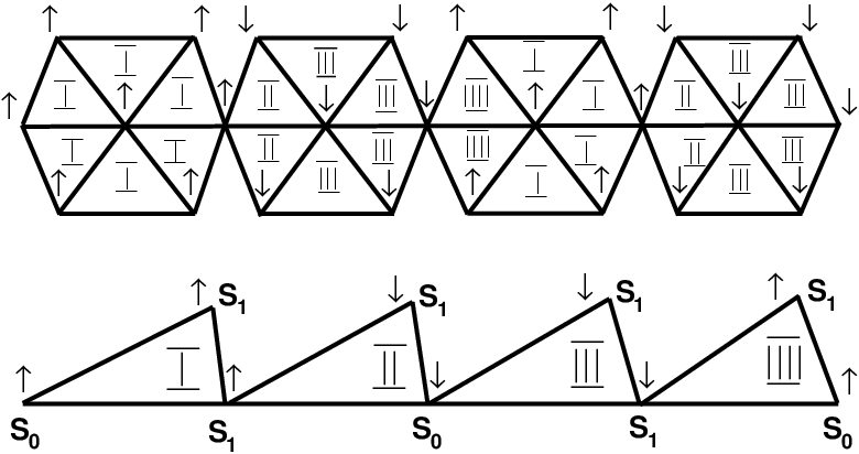
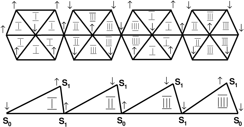
In the following plots we can see bifurcation points and one period doubling phenomena between bifurcation points represented on figure 3.12 a is the magnetization for the central vertex lattice with temperature , b is the magnetization for the corner vertex lattice with temperature , c is the average magnetization for the lattice with temperature .

Thus we’ve got magnetization plateaus, bifurcation points, doubling behavior, modulated phases for multiple exchange model where is taken into account both ferromagnetic and antiferromagnetic interactions. When we are changing interaction parameters or as the same the density in the physical limits got from experiment[70] close to we see magnetization plateaus, bifurcation points, doubling behavior, modulated phases at low temperatures. fig. 3.8,3.9,3.12.
Chapter 4 Face-cubic Model 11 1 The results considered in this chapter are published in Ref. [81].
Cubic symmetry plays a significant role in many types of phase transitions and critical phenomena. Still in 70-s various models possessing cubic symmetry have been introduced to determine the nature of the displacive phase transitions in perovskites [131, 132]. Magnetic phenomena in cubic crystals are also affected by the lattice structure. For instance, in the crystalline solids with cubic–symmetric lattices (Fe, Ni, etc.) it leads to the modification of the magnetic exchange interaction giving rise to additional contributions to the conventional O(N)-symmetric Heisenberg Hamiltonian. The simplest contribution of the underlying cubic symmetry is the single-ion anisotropy of the form . During the last three decades different aspects of this issue have been the subject of various investigations.
In the framework of the field–theoretical approach to critical phenomena modelling of effects of cubic symmetry is usually performed in terms of continuous-spin Landau-Ginzburg effective Hamiltonian with cubic anisotropy, i.e. the - theory with an additional cubic term which breaks explicitly the O(N) invariance to a residual discrete cubic symmetry [133] - [138]:
| (4.1) |
where is a continuous N-component local vector order parameter, and is inverse temperature. The spin orientations, orthogonal to faces of an -dimensional hypercube will be favorable for , whereas positive values of favor the orientations toward the corners.
This model received numerous important applications, among which are such as the oxygen ordering in YBaCu3O6+x [134], one of the most studied high-Tc superconductor; the buckling instability of confined colloid crystal layer [135]; the micellar binary solution of water and amphiphile [136] etc. The two–dimensional case has been recently intensively studied within the framework of renormalization group technique in the space of fixed dimensionality up to five–loop approximation [137, 138]. The model was found to have four fixed points: the Gaussian one, the Ising one with N decoupled components, the O(N)–symmetric and the cubic fixed point. Analogous calculations were made for , as well revealing some peculiar type of cubic fixed point for corresponding to specific anisotropic mode of the critical behavior [139]-[142]. The surface critical behavior of the model was also studied [143]. It has been recently shown that the behavior of the spherical many–spin magnetic nanoparticle with surface anisotropy may be modelled by an effective single macro–spin with cubic anisotropy terms in the effective energy [144].
Another class of lattice cubic–symmetric spin models was introduced by Kim, Levy and Uffer in Ref. [145] to explain the tricritical–like behavior of cubic rare–earth compounds, particularly holmium antimonide, HoSb [145]-[150]. Projecting the pair exchange interaction onto the sixfold degenerated ground-state manifold of Ho3+ ion they arrived at the following effective Hamiltonian:
| (4.2) |
where the classical spin variables are the unit vectors restricted to have orientations, orthogonal to the faces of the cube and the sum is going over all the pairs of nearest–neighbor sites. Generalization for component spin is obvious: each spin can assume orientations:
| (4.3) |
This model is known as the Face-cubic model. It is connected to the continuous cubic model of Eq. (5.1) via the limit of strong anisotropy . In a similar way one can also consider quadrupolar pair interaction terms and obtain the following Hamiltonian provided all interactions are homogenous [147, 148]:
| (4.4) |
It is easy to see that Hamiltonian (4.4) can be represented in terms of two sets of discrete variables: a Potts–like determining which component of is non-zero and an Ising–like, corresponding to the sign of the component. Indeed,
| (4.5) |
where and . Therefore we have
| (4.6) |
Formally we can enlarge the Hamiltonian (4.4) up to the interaction terms of higher power of the :
| (4.7) |
For arbitrary finite this expression leads to the same Hamiltonian that of Eq. (4.6) with and . At the Hamiltonian (4.7) reduced to the – state Potts model; corresponds to two decoupled – state Potts model, and at one obtains the Ashkin–Teller model. Variational renormalization–group study of the pure and diluted – component face–cubic model in two dimensions has revealed existence of four competing possible types of critical behavior corresponding to – state Potts model, – state Potts model, Ising model and special ”cubic” fixed point [149, 150]. It was also found that at the transitions are continuous and critical behavior of the discrete face–cubic model belongs to the O(N)-model universality class. For the Ashkin–Teller–like behavior occurs and for transitions are of first order. There are also early results obtained within the mean–field (MF) theory [145] and using the Bethte–Peirels (BP) approximations and high–temperature series [146] for the case when only dipolar pair interactions are included . In the BP approximation the critical value of spin component , above which transitions are of the first order was found to be given by
| (4.8) |
where is the coordination number of the lattice. The limit corresponds to the MF solution and gives . In Ref. [146] the high–temperature series for – component face–cubic model on three dimensional fcc lattice were constructed up to 5-th order, from which authors obtained , whereas Eq. (4.8) gives us Moreover, although the MF solution of cubic model predicted the tricritical like behavior [145], the BP approximation showed that it is not the case [146]. Only inclusion of single–ion–anisotropy terms, quadrupolar pair interactions and crystal fields may drive the system tricritical [147].
4.1 Recursive Methods, Cayley Tree and Bethe Lattice
Among the vast variety of statistical mechanics lattice models with strong local interactions only very limited amount allows exact solutions. These exact solutions are known only for low–dimensional systems, more precisely for and ; most of exact solutions for two–dimensional systems are known only in the absence of the external field and/or for the special choice of model parameters [92]. Well known conventional approximate methods like MF theory and BP approximation in general can provide only more or less qualitatively satisfactory picture and in some cases they just fail. That is why the quest for the alternative approaches, which can provide more reliable results for the thermodynamics of lattice models is very important.

The recursive lattices are of twofold interest. On the one hand, the models, defined on a recursive lattices can be considered as an independent original area of research in which the powerful methods of dynamical systems theory and fractal geometry are successfully exploited for determining the thermodynamical properties of the statistical mechanics models. On the other hand, recursive lattices provide a specific kind of approximate treatment of many–particle systems physics. In the heart of these approximations not the simplification of the character or/and strength of the interaction between the system elements, but the modification of the topology of the underlying lattice lies. This modification in most cases consist in the replacement of the regular periodic ”physical” lattice by a recursive one, constructed by the certain algorithm and possessing the self–similarity, maintaining all interaction unchanged. For the large class of lattice models with commuting variables (”classical models”) this approach leads to the exact solution of the statical mechanics problem in terms of the theory of dynamical systems or, more precisely, in terms of discrete maps. The solution formally is rather similar to that which corresponds to conventional BP approximation but, in contrast to the latter, it is the exact solution for the lattice endowed with the recursive structure provided the boundary sites are properly taken into consideration. It was argued that in some cases, particularly in the models where multi–site interactions are presented [73, 87, 80] the recursive lattice approximation gives more reliable results than conventional BP [86].
The simplest example of recursive lattices is a Cayley tree, the self-similar graph, which contains no cycles. In order to construct a Cayley tree one should start with a central site . At the first step this site should be connected by links with others, which constitute the first shell or the first generation of the Cayley tree. The second shell of the Cayley tree is constructed by repeating this procedure for all sites of the first shell: each of the sites belonging to the first shell connects to the new sites. Thus, the second shell contains sites. Accomplishing this construction for n steps one arrives at the recursive connected graph, which contains no cycles and is called the Cayley tree with coordination number and generations (shells) (Fig. 4.1). As the number of sites in -th shell is the total number of sites then
| (4.9) |
Thus, each site of the Cayley tree has coordination number equal to except the sites on the last shell which have only one neighbor. The peculiar property of the Caylet tree is the large amount of boundary sites which even in the thermodynamical limit comprise a finite fraction of the total number of sites
| (4.10) |
This feature causes anomalous properties of the statistical mechanics systems on the full Cayley tree. For instance, in Ising model there is no zero field magnetization, whereas the derivations of free energy with respect to the external field exhibit singular behavior [151] - [154].
The Bethe lattice is an object intimately linked to the Cayley tree but, in contrast to the latter, it is devoid of the complications which arise from the boundary sites. When one deals with the Bethe lattice the general structure and topology of the Cayley tree are preserved whereas only contributions from the bulk sites lying deep inside the Cayley tree are taken into consideration. In this regard the Bethe lattice is the interior of the Cayley tree [92, 155]. Dealing with the Bethe lattice we suppose the underlying Cayley tree to be large enough to achieve thermodynamical limit and consider only the sites situated far away from a boundary. One can regard these sites as a uniform lattice with coordination number .
An undeniable advantage of the Bethe lattice is the possibility of exact solutions for many types of statistical mechanics problems. A large amount of problems of the theory of magnetism, macromolecule physics, lattice gauge theory, self–organized criticality, dynamical mean–field theory (DMFT) and general questions of statistical mechanics like zeroes of partition functions have been successfully considered on Bethe or Bethe-like lattices, revealing many interesting exact results and deep connections between the theory of dynamical systems and statistical mechanics [151] - [164].
4.2 Face-cubic Model on Planar Graphs
It is possible to calculate exactly the partition function of the -model on Cayley tree in case of the absence of external field. Let us consider the partition function of the model without external field on arbitrary planar graph
| (4.11) |
As in the case of Potts model [165] one can represent it in the following way:
| (4.12) |
where . Then summing out over the all we obtain that
| (4.13) |
where the second sum is going over all spanning graphs of the underlying planar graph and is the 0-th Betti’s number of which coincides with the number of connected components of and the product is over all links belonging to . Using the identity one can represent Eq. (4.13) in terms of double power series associated with the underlying lattice provided latter is a planar graph:
| (4.14) |
where is the edges number in the graph and all assume values 0 or 1. So, for each spanning subgraph of planar graph we obtain a partition function of 2-state Potts model:
| (4.15) | |||||
where the second sum is going over all subgraph of Thus, we have succeeded in representing the partition function of the - model given by Hamiltonian (4.6) in terms of double power series associated with the underlying lattice provided the latter is a planar graph. As in case of ordinary spin Potts model one can make -expansions for -model with the aid of Eq. (4.15). For instance, for the two–dimensional square lattice one obtains
| (4.16) | |||||
Now we can use the well known relations between the topological invariants of graphs [166] to rewrite Eq. (4.15) in another way suitable for our further purposes. Applying the Euler theorem to planar graph we get
| (4.17) |
where the first Betti’s number coincides with the number of independent cycles of and is the number of sites. Therefore
| (4.18) |
Partition function for -model in the form of Eq. (4.18) can easily be calculated in case of the so-called forests, the planar graphs, which contain no cycles. Connected part of forest is called tree. Let us suppose that we have a tree with sites and edges. Then Eq.(4.18) takes the form
| (4.19) | |||||
where are the binomial coefficients and the sum is going over all subgraphs with given volume . With the aid of Newton’s binom we obtain
| (4.20) |
If is the Cayley tree then and we will have
| (4.21) |
Thus, the free energy per site for -model on Cayley tree is
| (4.22) |
It is noteworthy that this result is in full agreement with that obtained by Aharony for one–dimensional model by transfer–matrix technique [148]. Indeed, a one–dimensional chain can be regarded as a ”tree” in the sense mentioned above. Thus, the free energy of the model on a Cayley tree in a thermodynamic limit is continuous for all . Formally it coincides with that for one–dimensional systems where the continuity is really the case. But, as is known, the BP approximations for the lattice model with an arbitrary number of component solves exactly the problem on a Cayley tree [159]. Therefore the model on a Cayley tree must possess a finite critical temperature as predicted by BP approximation [146]. The origin of this peculiar properties of the Cayley tree was revealed by Eggarter [151] on the example of Ising model. He argued that the equivalence of all sites in the thermodynamic limit, which is one of the key points of BP approximation, breaks down for the sites of the Cayley tree which are situated close to the surface. As appears from Eq. (4.10) these sites comprise rather large fraction of the sites of the Cayley tree and, thus, they determine the behavior of all thermodynamic quantities to a great extent.
However, even though no phase transitions in the thermodynamic limit occur at the value of critical temperature predicted by the BP method the value of the order parameter (magnetization etc.) in the interior of the lattice, i. e. for the region far from the surface, which is generally called ”Bethe lattice”, will undergo jumps from zero to its BP value when the temperature is below . In order to illustrate it we will use the technique of dynamical system theory, which becomes a powerful tool for investigating various physical problems on recursive lattices.
4.3 Recursive Method for Face Cubic model on Bethe lattice.
Many statistical systems defined on the recursive lattices are famous for the possibility of exact solution in terms of dynamical system theory. In the heart of these exact solutions the self-similarity of recursive lattices lies. For instance, if we cut apart the Cayley tree at the central site it will give q identical branches each of which is the same Cayley tree with the number of generation decreased by 1. Using this fact one can establish the connection between the partition function of a model defined on the Cayley tree containing n shells with the partition function of the same model defined on the Cayley tree containing n-1 shells. Therefore, the thermodynamical problem is reformulated in terms of discrete maps, given by recurrent relations. Let us introduce a symmetry breaking field into Hamiltonian (4.6). The field can be considered as a uniform magnetic field pointing along the first coordinate axis . The corresponding interaction Hamiltonian is of the conventional Zeeman type:
| (4.23) |
which leads to the following form of the -model Hamiltonian in the field:
| (4.24) |
where . Hereafter we pass from the Cayley tree to the Bethe lattice having in mind one of the ways mentioned in Section II. Thus, we should no longer care about boundary sites and boundary conditions. According to that one can represent the partition function of the -model on the Bethe lattice in the following form:
| (4.25) |
where and are the variables of the spin in the central site and refers to a partition function of individual branch:
Each branch, in its turn, can be cut at the site which was previously connected to the central one. This will give us q-1 identical branches being the Bethe lattices with n-1 generations. Thus, the connection between and is
| (4.26) |
Here we obtain the system of recursion relations but, in fact, only three of them are independent as all for are identical. So, from (4.26) we have
| (4.27) | |||
| (4.28) | |||
| (4.29) |
where stand for any partition functions corresponding to the individual branch with whose direction is non collinear with the first coordinate axes. Introducing the variables
| (4.30) | |||
we obtain the system of two recurrent relations
| (4.31) | |||
with
| (4.32) | |||
where the following notations are adopted
| (4.33) | |||||
In this approach statistical averages of all physical quantities can be expressed in terms of and variables defined by Eq. (4.31). For instance, when the total number of spins is the magnetization along the first coordination axis which is the thermal average of the following form:
| (4.34) |
in terms of and are expressed as
| (4.35) |
provided all sites of the lattice are equivalent. It is easy to see that this quantity plays the role of an order parameter of Ising universality class. Another order parameter belonging to the –state Potts universality class is
| (4.36) |
which also can be regarded as a ”quadrupolar” moment . Thus
| (4.37) |
The order parameters and define the three possible
phases of the model in case of the ferromagnetic
couplings, i.e. , provided external magnetic field is vanished:
(a) disordered (paramagnetic) phase: ,
(b) ferromagneticaly ordered phase: ,
(c) partially ordered (quadrupolar) phase: ,
4.4 Investigations of phase transitions in terms of dynamical systems theory
In order to obtain physical results one must implement an iterative procedure for the RR (4.32). Namely, starting from the random initial conditions one uses the simple iterations scheme and examines the behavior of physical quantities after a large number of iterations [156]. In a simplest case the iterative sequence converges to a fixed point , which is defined by
This situation is inherent to the ferromagnetic case when both and are positive. As can easily be seen from Eqs. (4.34) - (4.37), when the magnetization and quadrupolar moment of the system take values and respectively, then the corresponding fixed point of the RR (4.32) is the following, provided :
Thus, according to the properties of different phases of the
ferromagnetic
model one can establish the connection between them and the
classification of the possible types of fixed points:
(a) disordered (paramagnetic) phase:
(b) ferromagneticaly ordered phase:
(c) partially ordered (quadrupolar) phase:
The condition
leads to , which means that the probability
of spin ”up” is equal to the probability of spin ”down” which is really the
case in paramagnetic phase.
Applying the simple iterative scheme to Eqs. (4.31), (4.35)
and (4.37) one can obtain the plots of magnetization processes
( vs. at fixed values of ) as well as the zero field
magnetization and quadrupolar moment of the system.
 |
 |
In Fig. 4.2 one can see the temperature dependencies of the order parameters of the -model on Bethe lattice with coordination number and . As is obviously seen from Fig. 4.2(a) in this case the zero field magnetization is always continuous, whereas the behavior of is quite different. Depending on the value of ratio the curve could be continuous or can include one first order transition point. In Fig. 4.2(b) one can see that at small values of only the one phase transition occurs from disordered phase to ferromagnetic phase omitting the partially ordered phase. This transition is of the second order until reaches some intermediate value above which one can see a discontinuity in the order parameter at critical temperature corresponding to the transition between disordered and ferromagnetic phases. At large values of the system undergoes successively two phase transitions at temperatures and , the larger one corresponds to the transition between disordered and quandrupolar phases, the lower one – to the transitions from quandrupolar to ferromagnetic. Within this region of the values of one can see the second order transition from disordered phase into ”quadrupolar” phase and the further first order transition to the ferromagnetic phase. However, beginning with some value of the transition between quadrupolar and ferromagnetic phases becomes continuous.

In order to complete the picture of the phase structure of the model under consideration at we plot a phase diagram by separating the regions of the fixed points of different kinds of the RR from Eq. (4.32) in the -plane. One can see in Fig. 4.3 that in case of , at the phase transition from disordered to ferromagnetic phase is of the second order. This feature maintains up to , where one can notice the tricritical point separating the region of continuous transitions from the region of the first order transitions. The line of the second order phase transitions between disordered and quadrupolar phases merges the line of transitions between disordered and ferromagnetic phase at , the latter, in its turn, again becomes of the second order at and for large values of it becomes parallel to the axis which means that the transition temperature between quadrupolar and ferromagnetic phases is unaffected by the value of beginning with .
 |
 |

The situation is quite different for . In Fig. 4.4 the plots of zero field magnetization and quadrupolar moment for and are presented. In this case both and are discontinuous at the critical temperatures. Moreover, this feature is preserved for for all values of , whereas becomes continuous after . the corresponding phase diagram is presented in Fig. 4.5. Here one can see a triple point at where the merging of the three lines of the first order transitions takes place. There is also a tricritical point at which separates the region of the first and the second order phase transitions on the line between quadrupolar and ferromagnetic phases. The line, as in case of , goes to plateau beginning with , so the transition temperature again does not depend on for . In general, for the pase diagrams of the model under consideration have the same topology as in case of . The main feature is the decrease of the distance between triple and tricritical points with the increase of the . So, for one can obtain that this distance is of order with . Apparently, they have never shrunk to a single point at finite values of , but it could be the case when . The value of critical spin component number at which the phase transitions become of the first order at in the Face-cubic model on Bethe lattice is exactly equal to 3, which coincides with the mean–field results at , but, in contrast to that, on Bethe lattice this value is unaffected by the value of coordination number . Obviously, this is the direct consequence of the fact, that the Bethe–Pierels approximation become exact on the Bethe lattice.
Chapter 5 Azimuthal Asymmetries in DIS as a Probe of Intrinsic Charm Content of the Proton 11 1 The results considered in this chapter are published in Refs. [84, 85].
The notion of the intrinsic charm (IC) content of the proton has been introduced over 25 years ago in Refs [41, 42]. It was shown that, in the light-cone Fock space picture [167, 168], it is natural to expect a five-quark state contribution to the proton wave function. The probability to find in a nucleon the five-quark component is of higher twist since it scales as where is the -quark mass [169]. This component can be generated by fluctuations inside the proton where the gluons are coupled to different valence quarks. Since all of the quarks tend to travel coherently at same rapidity in the bound state, the heaviest constituents carry the largest momentum fraction. For this reason, one would expect that the intrinsic charm component to be dominate the -quark production cross sections at sufficiently large Bjorken . So, the original concept of the charm density in the proton [41, 42] has nonperturbative nature and will be referred to in the present paper as nonperturbative IC.
A decade ago another point of view on the charm content of the proton has been proposed in the framework of the variable flavor number scheme (VFNS) [43, 44]. The VFNS is an approach alternative to the traditional fixed flavor number scheme (FFNS) where only light degrees of freedom ( and ) are considered as active. It is well known that a heavy quark production cross section contains potentially large logarithms of the type whose contribution dominates at high energies, . Within the VFNS, these mass logarithms are resummed through the all orders into a heavy quark density which evolves with according to the standard DGLAP [170, 171, 172] evolution equation. Hence the VFN schemes introduce the parton distribution functions (PDFs) for the heavy quarks and change the number of active flavors by one unit when a heavy quark threshold is crossed. We can say that the charm density arises within the VFNS perturbatively via the evolution and will call it the perturbative IC.
Presently, both perturbative and nonperturbative IC are widely used for a phenomenological description of available data. (A recent review of the theory and experimental constraints on the charm quark distribution can be found in Refs. [173, 174]. See also Appendix 5.5 in the present thesis). In particular, practically all the recent versions of the CTEQ [45] and MRST [46] sets of PDFs are based on the VFN schemes and contain a charm density. At the same time, the key question remains open: How to measure the intrinsic charm content of the proton? As mentioned in Introduction, the main theoretical problem is that production cross sections are not perturbatively stable.
In the present thesis we investigate the possibility to measure the charm content of the proton using the azimuthal asymmetries in heavy quark leptoproduction. For this purpose we calculate the IC contribution to azimuth-dependent process:
| (5.1) |
Neglecting the contribution of boson as well as the target mass effects, the cross section of the reaction (5.1) for unpolarized initial states may be written as
| (5.2) | |||
The quantity measures the degree of the longitudinal polarization of the virtual photon in the Breit frame [176],
| (5.3) |
and the kinematic variables are defined by
| (5.4) |
The cross sections in Eq. (5.2) are related to the structure functions as follows:
| (5.5) |
where and .

In Eq. (5.2), is the usual cross section describing heavy quark production by a transverse (longitudinal) virtual photon. The third cross section, , comes about from interference between transverse states and is responsible for the asymmetry which occurs in real photoproduction using linearly polarized photons [34, 35, 37]. The fourth cross section, , originates from interference between longitudinal and transverse components [176]. In the nucleon rest frame, the azimuth is the angle between the lepton scattering plane and the heavy quark production plane, defined by the exchanged photon and the detected quark (see Fig. 5.1). The covariant definition of is
| (5.6) | |||||
| (5.7) |
In Eqs. (5.4) and (5.6), and are the masses of the heavy quark and the target, respectively. Usually, the azimuthal asymmetry associated with the distribution, , is defined by
| (5.8) | |||||
where and the mean value of is
| (5.9) |
In Eq. (5.8), the quantities and are defined as
| (5.10) | |||||
| (5.11) |
Likewise, we can define the azimuthal asymmetry associated with the distribution,
:
| (5.12) | |||||
where
| (5.13) |
Remember that in most of the experimentally reachable kinematic range. Taking also into account that , we find:
| (5.14) |
So, like the cross section in the -independent case, it is the parameters and that can effectively be measured in the azimuth-dependent production.
In this paper we concentrate on the azimuthal asymmetry associated with the -distribution. We have calculated the IC contribution to the asymmetry which is described at the parton level by the photon-quark scattering (QS) mechanism given in Fig. 5.2. Our main result can be formulated as follows:
-
Contrary to the basic GF component, the IC mechanism is practically -independent. This is due to the fact that the QS contribution to the cross section is absent (for the kinematic reason) at LO and is negligibly small (of the order of ) at NLO.
As to the -independent cross sections, our parton level calculations have been compared with the previous results for the IC contribution to and presented in Refs. [38, 39]. Apart from two trivial misprints uncovered in [38] for , a complete agreement between all the considered results is found.
Since the GF and QS mechanisms have strongly different -distributions, we investigate the possibility to discriminate between their contributions using the azimuthal asymmetry . We analyze separately the nonperturbative IC in the framework of the FFNS and the perturbative IC within the VFNS.
The following properties of the nonperturbative IC contribution to the azimuthal asymmetry within the FFNS are found:
- •
The nonperturbative IC is practically invisible at low , but affects essentially the GF predictions at large . The dominance of the -independent IC component at large leads to a more rapid (in comparison with the GF predictions) decreasing of with growth of .
- •
Contrary to the production cross sections, the asymmetry in charm azimuthal distributions is practically insensitive to radiative corrections at . Perturbative stability of the combined GF+QS result for is mainly due to the cancellation of large NLO corrections in Eq. (5.11).
- •
pQCD predictions for the asymmetry are parametrically stable; the GF+QS contribution to is practically insensitive to most of the standard uncertainties in the QCD input parameters: , , and PDFs.
- •
Nonperturbative corrections to the charm azimuthal asymmetry due to the gluon transverse motion in the target are of the order of at and rapidly vanish at .
We conclude that the contributions of both GF and IC components to the asymmetry in charm leptoproduction are quantitatively well defined in the FFNS: they are stable, both parametrically and perturbatively, and insensitive (at ) to the gluon transverse motion in the proton. At large Bjorken , the asymmetry could be a sensitive probe of the nonperturbative IC.
The perturbative IC has been considered within the VFNS proposed in Refs. [43, 44]. The following features of the azimuthal asymmetry should be emphasized:
-
Contrary to the nonperturbative IC component, the perturbative one is significant practically at all values of Bjorken and .
-
The charm densities of the recent CTEQ and MRST sets of PDFs lead to a sizeable reduction (by about 1/3) of the GF predictions for the asymmetry.
We conclude that impact of the perturbative IC on the asymmetry is sizeable in the whole region of and, for this reason, can easily be detected.
Concerning the experimental aspects, azimuthal asymmetries in charm leptoproduction can, in principle, be measured in the COMPASS experiment at CERN, as well as in future studies at the proposed eRHIC [47, 48] and LHeC [49] colliders at BNL and CERN, correspondingly.
The paper is organized as follows. In Section 5.1 we analyze the QS and GF parton level predictions for the -dependent charm leptoproduction in the single-particle inclusive kinematics. In particular, we discuss our results for the NLO QS cross sections and compare them with available calculations. Hadron level predictions for are given in Section 5.2. We consider the IC contributions to the asymmetry within the FFNS and VFNS in a wide region of and . Some details of our calculations of the QS cross sections are presented in Appendix 5.3. An overview of the soft-gluon resummation for the photon-gluon fusion mechanism is given in Appendix 5.4. Some experimental facts in favor of the nonperturbative IC are briefly listed in Appendix 5.5.
5.1 Partonic Cross Sections
5.1.1 Quark Scattering Mechanism

The momentum assignment of the deep inelastic lepton-quark scattering will be denoted as
| (5.15) |
Taking into account the target mass effects, the corresponding partonic cross section can be written as follows [84]
| (5.16) | |||
In Eq. (5.16), we use the following definition of partonic kinematic variables:
| (5.17) |
In the massive case, the (virtual) photon polarization parameter, , has the form [84]
| (5.18) |
At leading order, , the only quark scattering subprocess is
| (5.19) |
The cross sections, (), corresponding to the Born diagram (see Fig. 5.2a) are:
| (5.20) | |||||
with
| (5.21) |
where is the quark charge in units of electromagnetic coupling constant.
To take into account the NLO contributions, one needs to calculate the virtual corrections to the Born process (given in Fig. 5.2c) as well as the real gluon emission (see Fig. 5.2b):
| (5.22) |
The NLO -dependent cross sections, and , are described by the real gluon emission only. Corresponding contributions are free of any type of singularities and the quantities and can be calculated directly in four dimensions.
In the -independent case, and , we also work in four dimensions. The virtual contribution (Fig. 5.2c) contains ultraviolet (UV) singularity that is removed using the on-mass-shell regularization scheme. In particular, we calculate the absorptive part of the Feynman diagram which has no UV divergences. The real part is then obtained by using the appropriate dispersion relations. As to the infrared (IR) singularity, it is regularized with the help of an infinitesimal gluon mass. This IR divergence is cancelled when we add the bremsstrahlung contribution (Fig. 5.2b). Some details of our calculations are given in Appendix 5.3.
The final (real+virtual) results for cross sections can be cast into the following form:
| (5.23) | |||||
| (5.24) | |||||
| (5.25) |
| (5.26) | |||
In Eqs. (5.23-5.26), , where is number of colors, while
| (5.27) |
The so-called ”plus” distributions are defined by
| (5.28) |
For any sufficiently regular test function , Eq. (5.28) gives
| (5.29) |
To perform a numerical investigation of the inclusive partonic cross sections, (), it is convenient to introduce the dimensionless coefficient functions ,
| (5.30) |
where is a factorization scale (we use ) and the variable measures the distance to the partonic threshold:
| (5.31) |
 |
 |
Our analysis of the quantity is given in Fig. 5.3. One can see that is negative at low () and positive at high (). For the intermediate values of , is an alternating function of .
Our results for the coefficient function at several values of are presented in Fig. 5.3. It is seen that is negative at all values of and . Note also the threshold behavior of the coefficient function:
| (5.32) |
This quantity takes its minimum value at :
. Let us analyze the numerical significance of the - and -distributions for the QS component. It is difficult to compare directly the and cross sections given by the usual functions (5.25) and (5.26) with the -independent contributions and described by the generalized functions (5.20) and (5.23). For this reason, we consider the Mellin moments of the corresponding quantities defined as
| (5.33) |
The Mellin transform of the Born level cross sections is trivial: . The Mellin moments of the NLO results have been calculated numerically. We use for the one-loop approximation with MeV, and GeV.
 |
 |
The left panel of Fig. 5.4 presents the ratio as a function of for several values of variable : and 100. One can see that this ratio is negligibly small (of the order of 1). Moreover, our analysis shows that the ratio is less than for all values of and . This implies that the photon-quark scattering contribution is practically -independent and, for this reason, we will neglect cross section in our further analysis.
In the right panel of Fig. 5.4, the -dependence of the ratio is given for the same values of . One can see that this ratio is of the order of 10-15 at small and sufficiently high . This fact indicates that the -distribution caused by the QS component may be sizable.
5.1.2 Comparison with Available Results
For the first time, the NLO corrections to the -independent IC contribution have been calculated a long time ago by Hoffmann and Moore (HM) [38]. However, authors of Ref. [38] don’t give explicitly their definition of the partonic cross sections that leads to a confusion in interpretation of the original HM results. To clarify the situation, we need first to derive the relation between the lepton-quark DIS cross section, , and the partonic cross sections, and , used in [38]. Using Eqs. (C.1) and (C.5) in Ref. [38], one can express the HM tensor in terms of ”our” cross sections and defined by Eq. (5.16) in the present paper. Comparing the obtained results with the corresponding definition of via the HM cross sections and (given by Eqs. (C.16) and (C.17) in Ref. [38]), we find that
| (5.34) | |||||
| (5.35) |
Now we are able to compare our results with original HM ones. It is easy to see that the LO cross sections (defined by Eqs. (37) in [38] and Eqs. (5.20) in our paper) obey both above identities. Comparing with each other the quantities and (given by Eq. (51) in [38] and Eq. (5.23) in this paper, respectively), we find that identity (5.34) is satisfied at NLO too. The situation with longitudinal cross sections is more complicated. We have uncovered two misprints in the NLO expression for given by Eq. (52) in [38]. First, the r.h.s. of this Eq. must be multiplied by . Second, the sign in front of the last term (proportional to ) in Eq. (52) in Ref. [38] must be changed 22 2 Note that this term originates from virtual corrections and the virtual part of the longitudinal cross section given by Eq. (39) in Ref. [38] also has wrong sign. See Appendix 5.3 for more details.. Taking into account these typos, we find that relation (5.35) holds at NLO as well. So, our calculations of and agree with the HM results.
Recently, the heavy quark initiated contributions to the -independent DIS structure functions, and , have been calculated by Kretzer and Schienbein (KS) [39]. The final KS results are expressed in terms of the parton level structure functions and . Using the definition of and given by Eqs. (7, 8) in Ref. [39], we obtain that
| (5.36) | |||
where and are defined by Eq. (5.16) in our paper and . To test identities (5.36), one needs only to rewrite the NLO expressions for the functions and (given in Appendix C in Ref. [39]) in terms of variables and . Our analysis shows that relations (5.36) hold at both LO and NLO. Hence we coincide with the KS predictions for the cross sections.
However, we disagree with the conclusion of Ref. [39] that there are errors in the NLO expression for given in Ref. [38] 33 3 In detail, the KS point of view on the HM results is presented in PhD thesis [40], pp. 158-160.. As explained above, a correct interpretation of the quantities and used in [38] leads to a complete agreement between the HM, KS and our results for -independent cross sections.
As to the -dependent DIS, pQCD predictions for the cross sections and in the case of arbitrary values of and are not, to our knowledge, available in the literature. For this reason, we have performed several cross checks of our results against well known calculations in two limits: and . In particular, in the chiral limit, we reproduce the original results of Georgi and Politzer [177] and Méndez [178] for and . In the case of , our predictions for and given by Eqs. (5.23,5.25) reduce to the QED textbook results for the Compton scattering of polarized photons [179].
5.1.3 Photon-Gluon Fusion
The gluon fusion component of the semi-inclusive DIS is the following parton level interaction:
| (5.37) |
Corresponding lepton-gluon cross section, , has the following decomposition in terms of the helicity cross sections:
| (5.38) |
where the quantity is defined by Eq. (5.3) with .
At LO, , the only gluon fusion subprocess responsible for heavy flavor production is
| (5.39) |

The cross sections, (), corresponding to the Born diagrams given in Fig. 5.5 have the form [180, 181]:
| (5.40) | |||||
| (5.41) | |||||
| (5.42) | |||||
| (5.43) |
where is defined by Eq. (5.21) and the following notations are used:
| (5.44) |
Note that the dependence vanishes in the GF mechanism due to the symmetry which, at leading order, requires invariance under [182].
As to the NLO results, presently, only -independent quantities and are known exactly [23]. For this reason, we will use in our analysis the so-called soft-gluon approximation for the NLO cross sections (see Appendix 5.4). As shown in Refs. [31, 35, 36], at energies not so far from the production threshold, the soft-gluon radiation is the dominant perturbative mechanism in the interactions.
5.2 Hadron Level Results
5.2.1 Fixed Flavor Number Scheme and Nonperturbative Intrinsic Charm
In the fixed flavor number scheme 44 4 This approach is sometimes referred to as the fixed-order perturbation theory (FOPT)., the wave function of the proton consists of light quarks and gluons . Heavy flavor production in DIS is dominated by the gluon fusion mechanism. Corresponding hadron level cross sections, , have the form
| (5.45) | |||||
| (5.46) |
where describes gluon density in the proton evaluated at a factorization scale . The lowest order GF cross sections, (), are given by Eqs. (5.41). The NLO results, , to the next-to-leading logarithmic accuracy are presented in Appendix 5.4.
We neglect the fusion subprocesses. This is justified as their contributions to heavy quark leptoproduction vanish at LO and are small at NLO [23].
In the FFNS, the intrinsic heavy flavor component of the proton wave function is generated by fluctuations where the gluons are coupled to different valence quarks. In the present paper, this component is referred to as the nonperturbative intrinsic charm (bottom). The probability of the corresponding five-quark Fock state, , is of higher twist since it scales as [169]. However, since all of the quarks tend to travel coherently at same rapidity in the bound state, the heaviest constituents carry the largest momentum fraction. For this reason, the heavy flavor distribution function has a more ”hard” -behavior than the light parton densities. Since all of the densities vanish at , the hardest PDF becomes dominant at sufficiently large independently of normalization.
Convolution of PDFs with partonic cross sections does not violate this observation. In particular, assuming a gluon density (where ), we obtain that the LO GF contribution to scales as at , where is defined by Eq. (5.46). In the case of Hoffman and Moore charm density (see below), the LO IC contribution is proportional to at . It is easy to see that, independently of normalizations, the IC contribution to be dominate over the more ”soft” GF component at large enough .
For the first time, the intrinsic charm momentum distribution in the five-quark state was derived by Brodsky, Hoyer, Peterson and Sakai (BHPS) in the framework of a light-cone model [41, 42]. Neglecting the transverse motion of constituents, they have obtained in the heavy quark limit that
| (5.47) |
where corresponds to a probability for IC in the nucleon: .
Hoffmann and Moore (HM) [38] incorporated mass effects in the BHPS approach. They first introduced a mass scaling variable ,
| (5.48) |
where . To provide correct threshold behavior of the charm density, the constraint was imposed where
| (5.49) |
Resulting charm distribution function, , has the following form in the HM approach:
| (5.50) |
with defined by Eq. (5.47). Corresponding hadron level cross sections for the production, , due to the heavy quark scattering (QS) mechanism, are
| (5.51) |
where the charm density . The LO and NLO expressions for the partonic cross sections are given by Eqs. (5.20) and (5.23-5.26), respectively.
Note also that, in the FFNS, the full cross section for the charm production, , is simply a sum of the GF and IC components:
| (5.52) |
 |
 |
 |
 |
 |
 |
Let us discuss the FFNS predictions for the hadron level asymmetry parameter defined by Eq. (5.11). Fig. 5.6 shows as a function of for several values of variable : and 100. We display both LO and NLO predictions of the GF mechanism as well as the analogous results of the combined GF+QS contribution. The azimuthal asymmetry due to the mere LO GF component is given by solid line. The NLO GF predictions are plotted by dashed line. The LO and NLO results of the total GF+QS contribution are given by dash-dotted and long-dashed lines, respectively. In our calculations, the CTEQ5M [183] parametrization of the gluon distribution function is used and a probability for IC in the nucleon is assumed. Throughout this paper, the value for both factorization and renormalization scales is chosen. In accordance with the CTEQ5M parametrization, we use GeV and MeV [183].
One can see from Fig. 5.6 the following basic features of the azimuthal asymmetry, , within the FFNS. First, as expected, the nonperturbative IC contribution is practically invisible at low , but affects essentially the GF predictions at large . Since, contrary to the GF mechanism, the QS component is practically -independent, the dominance of the IC contribution at large leads to a more rapid (in comparison with the GF predictions) decreasing of with growth of .
The most remarkable property of the azimuthal asymmetry is its perturbative stability. In Refs. [35, 36], the NLO soft-gluon corrections to the GF predictions for the asymmetry in heavy quark photo- and leptoproduction was calculated. It was shown that, contrary to the production cross sections, the quantity is practically insensitive to soft radiation. One can see from Fig. 5.6 in the present paper that the NLO corrections to the LO GF predictions for are about few percent at not large . This implies that large soft-gluon corrections to and (increasing both cross sections by a factor of two) cancel each other in the ratio with a good accuracy. In terms of so-called -factors, for , perturbative stability of the GF predictions for is provided by the fact that the corresponding -factors are approximately the same at not large : .
Comparing with each other the dash-dotted and long-dashed curves in Fig. 5.6, we see that the NLO corrections to the combined GF+QS result for are also small. In this case, three reasons are responsible for the closeness of the LO and NLO predictions. At small , where the nonperturbative IC contribution is negligible, perturbative stability of the asymmetry is provided by the GF component. In the large- region, where the IC mechanism dominates, the azimuthal asymmetry rapidly vanishes with growth of at both LO and NLO because the QS component is practically -independent, 55 5 Although the ratio is sizeable at sufficiently large , the absolute values of the quantities and become so small that it seems reasonable to consider the asymmetry as equally negligible at both LO and NLO and treat the predictions as perturbatively stable.. At intermediate values of , where both mechanisms are essential, perturbative stability of is due to the similarity of the corresponding -factors: 66 6 Note however that this similarity takes only place at intermediate values of where both GF and QS components are essential. In the low- and large- regions, the factors and are strongly different..
Another remarkable property of the azimuthal asymmetry closely related to fast perturbative convergence is its parametric stability 77 7 Of course, parametric stability of the fixed order results does not imply a fast convergence of the corresponding series. However, a fast convergent series must be parametrically stable. In particular, it must be - and -independent.. The analysis of Refs. [34, 36] shows that the GF predictions for the asymmetry are less sensitive to standard uncertainties in the QCD input parameters ( and PDFs) than the corresponding ones for the production cross sections. We have verified that the same situation takes also place for the combined GF+QS results.
Let us discuss how the GF predictions for the azimuthal asymmetry are affected by nonperturbative contributions due to the intrinsic transverse motion of the gluon in the target. Because of the relatively low -quark mass, these contributions are especially important in the description of the cross sections for charmed particle production.
To introduce degrees of freedom, , one extends the integral over the parton distribution function in Eq. (5.45) to -space,
| (5.53) |
The transverse momentum distribution, , is usually taken to be a Gaussian:
| (5.54) |
In practice, an analytic treatment of effects is usually used. According to Ref. [184], the -smeared differential cross section of the process (5.1) is a two-dimensional convolution:
| (5.55) |
The factor in front of in the r.h.s. of Eq. (5.55) reflects the fact that the heavy quark carries away about one half of the initial energy in the reaction (5.1).
Values of the -kick corrections to the LO GF predictions for the asymmetry in the charm production are shown in Fig. 5.6 by dotted curves. Calculating the -kick effect we use GeV. One can see that -smearing for is about - in the region of low and rapidly decreases at high .
In Fig. 5.7, the dependence of the asymmetry on the nonperturbative intrinsic charm content of the proton is presented. We plot the LO predictions for as a function of for several values of the variable and quantity describing a probability for IC in the nucleon. Dash-dotted curves describe the + contributions with and . Solid lines correspond to the case when . Comparing with each other Figs. 5.6 and 5.7, one can see that even a contribution of the nonperturbative IC to the proton wave function could be extracted from the asymmetry at large enough Bjorken .
 |
 |
 |
 |
 |
 |
5.2.2 Variable Flavor Number Scheme and Perturbative Intrinsic Charm
One can see from Eqs. (5.41) that the GF cross section contains potentially large logarithm, . The same situation takes also place for the QS cross section given by Eq. (5.23). At high energies, , the terms of the form dominate the production cross sections. To improve the convergence of the perturbative series at high energies, the so-called variable flavor number schemes (VFNS) have been proposed. Originally, this approach was formulated by Aivazis, Collins, Olness and Tung (ACOT) [185, 43].
In the VFNS, the mass logarithms of the type are resummed via the renormalization group equations. In practice, the resummation procedure consists of two steps. First, the mass logarithms have to be subtracted from the fixed order predictions for the partonic cross sections in such a way that in the asymptotic limit the well known massless coefficient functions are recovered. Instead, a charm parton density in the hadron, , has to be introduced. This density obeys the usual massless NLO DGLAP evolution equation with the boundary condition where . So, we may say that, within the VFNS, the charm density arises perturbatively from the evolution.
In the VFNS, the treatment of the charm depends on the values chosen for . At low , the production cross sections are described by the light parton contributions ( and ). The charm production is dominated by the GF process and its higher order QCD corrections. At high , the charm is treated in the same way as the other light quarks and it is represented by a charm parton density in the hadron, which evolves in . In the intermediate scale region, , one has to make a smooth connection between the two different prescriptions.
Strictly speaking, the perturbative charm density is well defined at high but does not have a clean interpretation at low . Since the perturbative IC originates from resummation of the mass logarithms of the type , it is usually assumed that the corresponding PDF vanishes with these logarithms, i.e. for . On the other hand, the threshold constraint implies that is not a constant but ”live” function of . To avoid this problem, several solutions have been proposed (see e.g. Refs. [186, 188]). In this paper, we use the so-called ACOT() prescription [186] which guarantees (at least at ) the correct threshold behavior of the heavy-quark-initiated contributions.
Within the VFNS, the -independent charm production cross sections have three pieces:
| (5.56) |
where the first and third terms on the right hand side describe the usual (unsubtracted) GF and QS contributions while the second (subtraction) term renders the total result infra-red safe in the limit . The only constraint imposed on the subtraction term is to reproduce at high energies the familiar partonic cross section:
| (5.57) |
Evidently, there is some freedom in the choice of finite mass terms of the form (with a positive ) in . For this reason, several prescriptions have been proposed to fix the subtraction term. As mentioned above, we use the so-called ACOT() scheme [186].
According to the ACOT() prescription, the lowest order -independent cross section is
| (5.58) | |||
where is the LO gluon-quark splitting function, , and the LO GF cross section is given by Eqs. (5.41). Remember also that and .
The asymptotic behavior of the subtraction terms is fixed by the parton level factorization theorem. This theorem implies that the partonic cross sections d can be factorized into process-dependent infra-red safe hard scattering cross sections d, which are finite in the limit , and universal (process-independent) partonic PDFs and fragmentation functions :
| (5.59) |
In Eq. (5.59), the symbol denotes the usual convolution integral, the indices and denote partons, and . All the logarithms of the heavy-quark mass (i.e., the singularities in the limit ) are contained in the PDFs and fragmentation functions while d are IR-safe (i.e., are free of the terms). The expansion of Eq. (5.59) can be used to determine order by order the subtraction terms. In particular, for the LO GF contribution to the charm leptoproduction one finds [43]
| (5.60) |
where describes the charm distribution in the gluon within the factorization scheme.
One can see from Eq. (5.60) that the azimuth-dependent GF cross sections and don’t have subtraction terms at LO because the lowest order QS contribution is -independent. For this reason, the -dependence within the VFNS has the same form as in the FFNS:
| (5.61) |
 |
 |
 |
 |
 |
 |
Fig. 5.8 shows the ACOT() predictions for the asymmetry parameter at several values of variable : and 100. For comparison, we plot also the LO GF predictions (solid curves). In the ACOT() case, we consider the CTEQ5M (dotted lines) and CTEQ4M (dashed curves) parametrizations of the gluon and charm densities in the proton. Corresponding values of the charm quark mass are GeV [183] (for the CTEQ5M PDFs) and GeV [187] (for the CTEQ4M PDFs). The default value of the factorization scale is .
One can see from Fig. 5.8 the following properties of the azimuthal asymmetry, , within the VFNS. Contrary to the nonperturbative IC component, the perturbative one is significant practically at all values of Bjorken and . The perturbative charm contribution leads to a sizeable decreasing of the GF predictions for the -asymmetry. In the ACOT() scheme, the IC contribution reduces the GF results for by about . The origin of this reduction is straightforward: the QS component is practically -independent.
The ACOT() predictions for the asymmetry depend weakly on the parton distribution functions we use. It is seen from Fig. 5.8 that the CTEQ5M and CTEQ4M sets of PDFs lead to very similar results for . Note that we give the CTEQ5M predictions at low only because of irregularities in the CTEQ5M charm density at large .
We have also analyzed how the VFNS predictions depend on the choice of subtraction prescription. In particular, the schemes proposed in Refs. [39, 188] have been considered. We find that, sufficiently above the production threshold, these subtraction prescriptions reduce the GF results for the asymmetry by approximately .
One can conclude that impact of the perturbative IC on the asymmetry is essential in the whole region of Bjorken and therefore can be tested experimentally.
5.3 Appendix A: Virtual and Soft Contributions to the Quark Scattering
In this Appendix we reproduce some results of Hoffmann and Moore for the -independent QS cross sections, and correct two misprints uncovered in Ref. [38]. We work in four dimensions, in the Feynman gauge and use the on-mass-shell renormalization scheme. We compute the absorptive part of the Feynman diagram (which is free of the UV divergences) and then restore the real part using the appropriate dispersion relations.
In the on-mass-shell scheme, the renormalized fermion self-energy vanishes like which means that the second and third diagrams in Fig. 5.2c do not contribute to the cross section when the external quark legs are on-shell, . The first graph in Fig. 5.2c describes the NLO corrections to the quark-photon vertex function:
| (5.62) |
where while and are the quark electromagnetic formfactors. At the lowest order .
The virtual lepton-quark cross section, , is obtained from the interference term between the virtual and the Born amplitude. The result can be written in terms of the electromagnetic formfactors as:
| (5.63) |
Taking into account the definition of the HM cross sections, and , given by Eqs. (5.34), (5.35) and (5.16), we find that corresponding virtual parts are:
| (5.64) |
where and are the NLO corrections to the electromagnetic formfactors. For the NLO HM cross sections, and , we use exactly the same notations as in Ref. [38].
In the on-mass-shell renormalization scheme, the renormalized vertex correction vanishes as the photon virtuality goes to zero, . This is a consequence of the Ward identity and the fact that the real photon field (like the massive fermion one) is unrenormalized in first order QCD. To satisfy the condition automatically, we should use for the dispersion relation with one subtraction. The second formfactor, , has no singularities. For this reason, we use for the dispersion relation without subtractions:
| (5.65) |
Calculating the imaginary parts of the formafactors and restoring their real parts with the help of Eqs. (5.65) yields
| (5.66) | |||||
| (5.67) |
In Eqs. (5.66) and (5.67), , where is number of colors, and is defined by Eq. (5.27). Taking into account that , we see that Eqs. (5.66, 5.67) reproduce the textbook QED results.
It is now straightforward to obtain the virtual contribution to the longitudinal cross section. Combining Eqs. (5.64) and (5.67) yields:
| (5.68) |
Comparing the above result with the corresponding one given by Eq. (39) in Ref. [38], we see that the HM expression for has opposite sign. Note also that this typo propagates into the final result for given by Eq. (52) [38].
Calculation of the bremsstrahlung contribution to the longitudinal cross section, , is also straightforward. We coincide with the HM result for given by Eq. (49) in Ref. [38]. However there is one more misprint in the HM expression for : the r.h.s of Eq. (52) [38] should be multiplied by .
In the case of , the situation is slightly more complicated due to the need to take into account the IR singularities. One can see from Eq. (5.66) that has an IR divergence which is regularized with the help of an infinitesimal gluon mass . This singularity is cancelled when one adds the so-called soft contribution originating from the real gluon emission. For this purpose we introduce another infinitesimal parameter , . The full bremsstrahlung contribution, , can then be splitted into the soft and hard pieces as follows:
| (5.69) |
where is the Heaviside step function. The soft cross section should be calculated in the eikonal approximation, , taking into account the infinitesimal gluon mass . As a result, the sum of the virtual and soft contributions is IR finite:
| (5.70) | |||
Adding to the above expression the hard cross section defined by Eq. (5.69), we reproduce in the limit the full result for given by Eq. (51) in Ref. [38].
5.4 Appendix B: NLO Soft-Gluon Corrections to the Photon-Gluon Fusion
This Appendix provides an overview of the NLO soft-gluon approximation for the photon-gluon fusion mechanism. We present the final results for the parton level cross sections to the next-to-leading logarithmic (NLL) accuracy. More details can be found in Refs. [31, 35, 36].
To take into account the NLO contributions to the GF mechanism, one needs to calculate the virtual corrections to the Born process (5.39) and the real gluon emission:
| (5.71) |
The partonic invariants describing the single-particle inclusive (1PI) kinematics are
| (5.72) |
where is defined by and measures the inelasticity of the reaction (5.71). The corresponding 1PI hadron level variables describing the reaction (5.1) are
| (5.73) |
The exact NLO calculations of the unpolarized heavy quark production in [21, 22], [23], and [24, 25, 26, 27] collisions show that, near the partonic threshold, a strong logarithmic enhancement of the cross sections takes place in the collinear, , and soft, , limits. This threshold (or soft-gluon) enhancement has universal nature in the perturbation theory and originates from incomplete cancellation of the soft and collinear singularities between the loop and the bremsstrahlung contributions. Large leading and next-to-leading threshold logarithms can be resummed to all orders of perturbative expansion using the appropriate evolution equations [28, 29, 30]. The analytic results for the resummed cross sections are ill-defined due to the Landau pole in the coupling strength . However, if one considers the obtained expressions as generating functionals of the perturbative theory and re-expands them at fixed order in , no divergences associated with the Landau pole are encountered.
Soft-gluon resummation for the photon-gluon fusion has been performed in Ref. [31] and checked in Refs. [35, 36]. To NLL accuracy, the perturbative expansion for the partonic cross sections, ddd (), can be written in a factorized form as
| (5.74) |
with the Born level distributions given by
| (5.75) | |||||
| (5.76) | |||||
| (5.77) | |||||
| (5.78) |
Note that the functions in Eq. (5.74) originate from the collinear and soft limits. Radiation of soft and collinear gluons does not affect the transverse momentum of detected particles and therefore the azimuthal angle . For this reason, the functions are the same for all helicity cross sections (). At NLO, the soft-gluon corrections to NLL accuracy in the scheme are
| (5.79) | |||||
where we use . In Eq. (5.79), and , where is number of colors, while i with . The single-particle inclusive ”plus“ distributions are defined by
| (5.80) |
For any sufficiently regular test function , Eq. (5.80) gives
| (5.81) |
In Eq. (5.79), we have preserved the NLL terms for the scale-dependent logarithms too. Note also that the results (5.77) and (5.79) agree to NLL accuracy with the exact calculations of the photon-gluon cross sections and given in Ref. [23].
To investigate the scale dependence of the results (5.745.79), it is convenient to introduce for the fully inclusive (integrated over and ) cross sections, (), the dimensionless coefficient functions defined by Eq. (5.30). Concerning the NLO scale-independent coefficient functions, only and are known exactly [23, 191]. As to the -dependent coefficients, they can by calculated explicitly using the evolution equation:
| (5.82) |
where , , are the cross sections resummed to all orders in and is the corresponding (resummed) Altarelli-Parisi gluon-gluon splitting function. Expanding Eq. (5.82) in , one can find [31, 35]
| (5.83) |
where is the first coefficient of the -function expansion and is the number of active quark flavors. The one-loop gluon splitting function is:
| (5.84) |
With Eq. (5.83) in hand, it is possible to check the quality of the NLL approximation against exact answers. As shown in Ref. [36], the soft-gluon corrections reproduce satisfactorily the threshold behavior of the available exact results for . Since the gluon distribution function supports just the threshold region, the soft-gluon contribution dominates the photon-hadron cross sections () at energies not so far from the production threshold and at relatively low virtuality .
5.5 Appendix C: Nonperturbative IC and Relevant Experimental Facts
The most clean probe of the charm quark distribution function (both perturbative and nonperturbative) is the semi-inclusive deep inelastic lepton-proton scattering, . To measure the nonperturbative IC contribution, one needs data on the charm production at sufficiently large Bjorken . The only experiment which has investigated the large domain is the European Muon Collaboration (EMC) [192] where the decay lepton spectra have been used to detect the produced charmed particles. In Ref. [193], a re-analysis of the EMC data on have been performed using the NLO results for both GF and QS components. The analysis [193] shows that a nonperturbative intrinsic charm contribution to the proton wave function of the order of is needed to fit the EMC data in the large region. This value of the nonperturbative IC is consistent with the estimates based on the operator product expansion [169]. Note however that the EMC data are of limited statistics and, for this reason, more accurate measurements of charm leptoproduction at large are necessary.
It is also possible to extract useful information on the IC from diffractive dissociation processes such as on a nuclear target. Comprehensive measurements of the and cross sections have been performed in the fixed target experiments NA3 at CERN [194] and E886 at FNAL [195]. According to the arguments presented in Refs. [196, 197, 198], the IC contribution is predicted to be strongly shadowed in the above reactions that is in a complete agreement with the observed nuclear dependence of the high Feynman component of the hadroproduction.
A non-vanishing five-quark Fock component leads to the production of open charm states such as and with large Feynman . This may occur either through a coalescence of the valence and charm quarks which are moving with the same rapidity or via hadronization of the produced and . As shown in Refs. [199, 200], a model based on the nonperturbative intrinsic charm naturally explains the leading particle effect in the and processes that has been observed at the ISR [201] and Fermilab [202, 203].
As to the high- hadroproduction of open bottom states like , corresponding cross sections are predicted to be suppressed as in comparison with the case of charm production. Evidence for the forward production in the collisions at the ISR energy was reported in Refs. [204, 205].
Rare seven-quark fluctuations of the type in the proton wave function can lead to the production of two [206] or a double-charm baryon state at large and low . Double events with a high combined have been detected in the NA3 experiment [207]. An observation of the double-charmed baryon with mean has been reported by the SELEX collaboration at FNAL [208].
Conclusion
We conclude by summarizing our main observations and results. In this thesis, some spin effects in QCD and recurrence lattices with multi-site exchanges are investigated. Our conclusions concerning the critical phenomena in the recurrence spin models with multi-site exchanges can be formulated as follows.
We have studied the Yang-Lee complex zeros of the partition function of the anti-ferromagnetic Potts model for biopolymer formulated on the recursive zigzag ladder with three-spin interaction. Using the dynamical system approach of multi-dimensional mapping, we have obtained the helix-coil pseudo-phase transitions in the thermodynamic limit. Taking into account a non-classical helix-stabilizing interaction, we describe the folding and unfolding processes for proteins and polypeptides. We have got also Arnold tongues with different winding numbers in the considered microscopic theory [78, 79].
Using the dynamical system approach to solid and fluid 3He films with MSE on the recurrent lattices, we have obtained magnetization curves with plateaus (at and ) and one period doubling [80, 82, 83]. We have taken into account two, three, four, five, and sixspin exchanges. Interaction parameters used in calculations were taken from experimental results.
We have also considered (on the Bethe lattice) the model with cubic symmetry containing both linear and quadratic spin-spin interactions. An expression for the free energy per spin in the thermodynamic limit was found. Then we have identified the different thermodynamic phases of the system (disordered, partially ordered and completely ordered) in the ferromagnetic case (, ). We have obtained the phase diagrams of the model which are found to be different for and . The case of contains three tricritical points. When , one tricritical and one triple points there exist [81].
Next direction of our activity are spin effects in QCD. We consider the azimuthal dependence in charm leptoproduction as a probe of the IC content of the proton. Our analysis is based on the fact that the GF and QS components have strongly different -distributions [85]. This fact follows from the NLO calculations of both parton level contributions. In the framework of the FFNS, we justify the most remarkable property of the hadron level azimuthal asymmetry: the combined GF+QS predictions for are perturbatively and parametrically stable. The nonperturbative IC contribution (resulting from the five-quark component of the proton wave function) is practically invisible at low , but affects essentially the GF predictions for the asymmetry at large Bjorken . We conclude that measurements of the asymmetry at large could directly probe the nonperturbative intrinsic charm [84].
Within the VFNS, charm density originates perturbatively from the process and obeys the DGLAP evolution equation. Presently, charm densities are included practically in all the global sets of PDFs like CTEQ and MRST. Our analysis shows that these charm distribution functions reduce dramatically (by about 1/3) the GF predictions for practically at all values of . For this reason, the perturbative IC contribution can easily be measured using the azimuthal -distributions in charm leptoproduction [84].
This dissertation is based on the material published in journals: Physics Letters A [79], Physical Review B [80], Physica A [81], International Journal of Modern Physics B [82], Proceedings of National Academy of Sciences of Armenia, Physics [83], Nuclear Physics B [84], Physical Review D [85]. Our main results are reported on conferences: Chaos and Supercomputers (Nor-Amberd, Armenia 2000), IX International Conference on Symmetry Methods in Physics (Yerevan, Armenia 2001), Stat. Mech. and Dynamic Systems (Nor-Amberd, Armenia 2003), ”Fizika-2000” Young Scientist’s Republic Conference (Yerevan, Armenia 2004) , Selected Topics in Theoretical Physics (Tbilisi, Georgia 2005), and discussed on seminars in Yerevan Physics Institute and ICTP (Trieste, Italy).
Acknowledgments
It is a pleasure to thank N.S. Ananikian and N.Ya. Ivanov for suggesting these very interesting research topics to me. I am also grateful to my other co-authors, R. Roger, V. Ohanyan, T. Arakelyan and R. Artuso, for the fruitful collaboration. Finally, I would like express my gratitude to all the members of the Theory Division of YerPhI for useful discussions.
Bibliography
- [1]
S.A. Goudschmidt, G.H. Uhlenbeck, Spinning electrons and the structure of
spectra,
Nature 117, pp. 264-265 (1926). - [2]
A. Martin, History of spin and statistics,
hep-ph/0209068 pp. 1-27 (2002). - [3]
S. Schael et al., Precision electroweak measurements on the Z resonance,
Phys. Rept. 427, 257-454 (2006). - [4]
J. Ellis, Polarization puts a New Spin on Physics,
hep-ph/0701049 pp. 1-14 (2006). - [5]
J. Erler, Low energy tests of the standard model with spin degrees of freedom,
hep-ph/0612030 pp.1-10 (2006). - [6]
E. Ising, Beitrag zur theorie des ferromagnetismus,
Z. Physik 31, pp. 253-258 (1925). - [7]
L. Onsager, Crystal statistics I. A two-dimensional model with an order disorder
transition,
Phys. Rev. 65, pp. 117-149 (1944). - [8]
A. Pelissetto and E. Vicari, Critical phenomena and renormalization-group
theory,
Phys. Rep. 368, pp. 549-727 (2002). - [9]
T. Castellani, A. Cavagna, Spin-Glass Theory for Pedestrians,
J. Stat. Mech. P05012 pp. 1-52 (2005). - [10]
M. Mezard, G. Parisi, M. Virasoro, Spin Glass Theory and Beyond,
World Scientific, Singapore (1987). - [11]
K.G. Wilson, Renormalization group and critical phenomena. 1. Renormalization group and the Kadanoff scaling picture,
Phys. Rev. B4, pp. 3174-3183 (1971). - [12]
K.G. Wilson, J. Kogut, The renormalization group and the expansion,
Phys. Rep. 12 pp. 75-200 (1974). - [13]
J. Zinn-Justin, Quantum Field Theory and Critical Phenomena,
3rd Edition, Clarendon Press, Oxford, 1996. - [14]
K.G. Wilson, Confinement Of Quarks,
Phys. Rev. D10, pp. 2445-2459 (1974). - [15]
K.G. Wilson, Quarks and strings on a lattice, in: A. Zichichi
(Ed.),
New Phenomena in Subnuclear Physics, Plenum Press, New York, 1975. - [16]
M. Creutz, Quarks, Gluons and Lattices,
Cambridge University Press, Cambridge, 1983. - [17]
I. Montvay, G. Münster, Quantum Fields on a Lattice,
Cambridge University Press, Cambridge, 1994. - [18]
M. Creutz, L. Jacobs, C. Rebbi, Monte Carlo computations in lattice gauge theories,
Phys. Rep. 95, pp. 201-282 (1983). - [19]
M. L. Mangano, P. Nason, and G. Ridolfi, Heavy-quark correlations in hadron collisions at next-to-leading order
Nucl. Phys. B373, pp. 295-345 (1992). - [20]
S. Frixione, M. L. Mangano, P. Nason, and G. Ridolfi, Heavy-quark correlations in photon-hadron collisions
Nucl. Phys. B412, pp. 225-259 (1994). - [21]
R. K. Ellis and P. Nason, QCD radiative corrections to the photoproduction of heavy quarks,
Nucl. Phys. B 312, pp. 551-570 (1989). - [22]
J. Smith and W. L. van Neerven, QCD corrections to heavy flavour photoproduction and
electroproduction,
Nucl. Phys. B 374, pp. 36-82 (1992). - [23]
E. Laenen, S. Riemersma, J. Smith, and W. L. van Neerven, Complete corrections to heavy-flavour structure functions in electroproduction,
Nucl. Phys. B 392, pp. 162-228 (1993). - [24]
P. Nason, S. Dawson, and R. K. Ellis, The total cross section for the production of heavy quarks in hadronic collisions,
Nucl. Phys. B 303, pp. 607-633 (1988). - [25]
P. Nason, S. Dawson, and R. K. Ellis, The one particle inclusive differential cross section for heavy quark production in hadronic
collisions,
Nucl. Phys. B 327, pp. 49-92 (1989). - [26]
P. Nason, S. Dawson, and R. K. Ellis,
,
Nucl. Phys. B 335, 260 (1990). - [27]
W. Beenakker, H. Kuijf, W. L. van Neerven, and
J. Smith, QCD Corrections to Heavy Quark Production In p
anti-p Collisions,
Phys. Rev. D 40, pp. 54-82 (1989). - [28]
H. Contopanagos, E. Laenen, and
G. Sterman, Sudakov factorization and resummation,
Nucl. Phys. B 484, pp. 303-330 (1997). - [29]
E. Laenen, G. Oderda, and G. Sterman, Resummation of threshold corrections for single particle inclusive
cross-sections,
Phys. Lett. B 438, 173-183 (1998). - [30]
N. Kidonakis, G. Oderda, and G. Sterman, Evolution of color exchange in QCD hard
scattering,
Nucl. Phys. B 531, 365-402 (1998). - [31]
E. Laenen and S. -O. Moch, Soft gluon resummation for heavy quark electroproduction,
Phys. Rev. D 59, 034027 pp.1-18 (1999). - [32]
N. Kidonakis, Next-to-next-to-next-to-leading-order soft-gluon corrections in hard-scattering processes near threshold,
Phys. Rev. D 73, 034001 pp.1-13 (2006). - [33]
N. Kidonakis, High order corrections and subleading logarithms for top quark production,
Phys. Rev. D 64, 014009 pp.1-21 (2001). - [34]
N. Ya. Ivanov, A. Capella, and A. B. Kaidalov, Single spin asymmetry in heavy flavor photoproduction as a test of
pQCD
Nucl. Phys. B586, pp. 382-396 (2000). - [35]
N. Ya. Ivanov, Perturbative stability of the QCD predictions for single spin asymmetry in heavy quark photoproduction,
Nucl. Phys. B 615, pp. 266-284 (2001). - [36]
N. Ya. Ivanov, Azimuthal asymmetries in heavy quark leptoproduction as a test of pQCD,
Nucl. Phys. B 666, 88-104 (2003). - [37]
N. Ya. Ivanov, P. E. Bosted, K. Griffioen, and
S. E. Rock, Single spin asymmetry in open charm photoproduction and decay as a test of pQCD
Nucl. Phys. B 650, pp. 271-289 (2003). - [38]
E. Hoffmann and R. Moore, Subleading Contributions To The Intrinsic Charm Of The Nucleon,
Z. Phys. C 20, 71-82 (1983). - [39]
S. Kretzer and I. Schienbein, Heavy quark initiated contributions to deep inelastic structure functions,
Phys. Rev. D 58, 094035 pp.1-12 (1998). - [40]
I. Schienbein, Heavy Quark Production in CC and NC DIS and The Structure of Real and Virtual Photons in NLO QCD,
hep-ph/0110292. - [41]
S. J. Brodsky, P. Hoyer, C. Peterson, and N. Sakai, The Intrinsic Charm Of The
Proton,
Phys. Lett. B 93, pp. 451-455 (1980). - [42]
S. J. Brodsky, C. Peterson, and N. Sakai, Intrinsic Heavy Quark
States,
Phys. Rev. D 23, pp. 2745-2757 (1981). - [43]
M. A. G. Aivazis, J. C. Collins, F. I. Olness, and
W. -K. Tung, Leptoproduction of heavy quarks. 2. A Unified QCD
formulation of charged and neutral current processes from fixed
target to collider energies,
Phys. Rev. D 50, pp. 3102-3118 (1994). - [44]
J. C. Collins, Hard scattering factorization with heavy quarks: A General treatment,
Phys. Rev. D 58, 094002 pp. 1-29 (1998). - [45]
J. Pumplin, D. R. Stump, J. Huston, H. L. Lai, P. Nadolsky,
and W. K. Tung, New generation of parton distributions with
uncertainties from global QCD analysis,
JHEP 07, 012, pp. 1-47 (2002). - [46]
A. D. Martin, R. G. Roberts, W. J. Stirling, and
R. S. Thorne, Physical gluons and high E(T) jets,
Phys. Lett. B 604, pp. 61-68 (2004). - [47]
A. Deshpande, R. Milner, R. Venugopalan, and
W. Vogelsang, Study of the fundamental structure of matter
with an electron-ion collider,
Ann. Rev. Nucl. Part. Sci. 55, pp. 165-228 (2005). - [48] See also http://www.bnl.gov/eic for information concernig the eRHIC/EIC project.
- [49]
J. B. Dainton, M. Klein, P. Newman, E. Perez, and
F. Willeke, Deep Inelastic Electron-Nucleon Scattering at the LHC,
hep-ex/0603016. - [50]
C. N. Yang and T. D. Lee, Statistical Theory of Equations of State and Phase Transitions. I. Theory of
Condensation,
Phys. Rev 87, pp. 404-409 (1952). - [51]
T. D. Lee and C. N. Yang, Statistical Theory of Equations of State and Phase Transitions. II. Lattice Gas and Ising Model,
Phys. Rev. 87, pp. 410-419 (1952). - [52]
P. W. Kasteleyn and C.M Fortuin, Phase transitions in lattice systems with random local properties,
J. Phys. Soc. Japan 26, (Suppl.)11 (1969); - [53]
C.M Fortuin and P. W. Kasteleyn, Random-cluster model. Introduction and relation to other models,
Physica 57, pp. 536-564 (1972); - [54]
J.Salas and A. D. Sokal, Transfer matrices and partition-function zeros for antiferromagnetic Potts models,
J. Stat. Phys. 104, pp. 609-699 (2001). - [55]
J.G. Brankov, Vl.V. Papoyan, V.S. Poghosyan, V.B.
Priezzhev, The totally asymmetric exclusion process on a ring:
Exact
relaxation dynamics and associated model of clustering transition,
Physica A 368, pp. 471-480 (2006). - [56]
U.H.E. Hansmann, Y. Okamoto, Finite-size scaling of helixcoil transitions in poly-alanine studied by multicanonical simulations,
J. Chem. Phys. 110, pp. 1267-1276 (1999). - [57]
N. A. Alves, U.H.E. Hansmann, Partition Function Zeros and Finite Size Scaling of Helix-Coil Transitions in a Polypeptide,
Phys. Rev. Lett. 84, pp. 1836-1839 (2000). - [58]
Y. Okamoto, U. H. E.Hansmann, Thermodynamics of Helix-Coil Transitions Studied by Multicanonical Algorithms ,
J. Phys. Chem. 99 pp. 11276-11287 (1995). - [59]
N. A. Alves and U.H.E. Hansmann, Yang-Lee zeros and the helix-coil transition in a continuum model of polyalanine,
Physica A292, pp. 509-518 (2001) - [60]
S. Coombes and P. C. Bressloff, Mode locking and Arnold tongues in integrate-and-fire neural oscillators,
Phys. Rev E60, pp. 2086-2096 (1999);
R. S. Mackay and C. Tresser, Transition to topological chaos for circle maps,
Physica D19, pp. 206-237 (1986). - [61]
C. N. Pace and Ch. Tanford, Thermodynamics of the unfolding of beta-lactoglobulin A in aqueous urea solutions between 5 and 55
degrees,
Biochemistry 7, pp. 198-213 (1968);
G. P. Privalov and P. L. Privalov, Problems and prospects in the microcalorimetry of biological macromolecules,
Methods Enzymol. 323, pp. 31-62 (2000). - [62]
A. Bakk, J. S. Høye, and A. Hassen, Apolar and polar solvation thermodynamics related to the protein unfolding process,
Biophysical Journal 82 pp. 713-719 (2002);
O. Collet, Four-states phase diagram of proteins,
Europhysics Letters 72 pp. 301-307 (2005). - [63]
O. Collet, Warm and cold denaturation in the phase diagram of a protein lattice model,
Europhysics Letters 53 pp. 93-99 (2001). - [64]
P.Bruscolini, C. Buzano, A. Pelizzola, M. Pretti, Bethe approximation for a model of polymer solvation,
Phys. Rev. E 64 050801(R) pp. 1-4 (2001). - [65]
D. J. Jacobs, S. Dallakyan, G. G. Wood, A.
Heckathorne, Network rigidity at finite temperature:
Relationships between thermodynamic stability, the nonadditivity of
entropy, and cooperativity in molecular systems,
Phys. Rev. E68, 061109 pp. 1-22 (2003). - [66] D. Mattise, The theory of magnetism (Harper and Row, New York) (1982).
- [67]
J. G. Bednorz and K. A. Müller, Possible high superconductivity in the Ba-La-Cu-O system,
Z. Phys. B64, pp. 189-193 (1986). - [68]
M. Roger, J. H. Hetherington, J. M. Delrieu, Magnetism in solid ,
Rev. Mod. Phys. 55, pp. 1-64 (1983);
H. Franco, R. Rapp and H. Godfrin, Nuclear Ferromagnetism of Two-Dimensional 3He,
Phys. Rev. Lett. 57, pp. 1161-1164 (1986);
H. Godfrin, R. Ruel and D. Osheroff, Experimental Observation of a Two-Dimensional Heisenberg Nuclear Ferromagnet,
Phys. Rev. Lett. 60, pp. 305-308 (1988). - [69]
H. Godfrin and R. E. Rapp, Two-dimensional nuclear magnets,
Adv. Phys. 44, pp. 113-186 (1995). - [70]
M. Roger, C.Bäuerle, Yu. M. Bunkov, A.-S. Chen and H.
Godfrin, Multiple-Spin Exchange on a Triangular Lattice: A
Quantitative Interpretation of Thermodynamic Properties of
Two-Dimensional Solid ,
Phys. Rev. Lett. 80, pp. 1308-1311 (1998). - [71]
H. Godfrin and D. D. Osheroff,Multiple-spin-exchange calculation of the T=0 properties of solid
3He,
Phys. Rev. B 38, pp. 4492-4503 (1988). - [72]
N. S. Ananikan, A. R. Avakian, and N. Sh. Izmailian, Phase diagrams and tricritical effects in the beg model,
Physica A 172, pp. 391-404 (1991). - [73]
N.S. Ananikian, S.K. Dallakian, B. Hu, Chaotic Properties of the Q-state Potts Model on the Bethe Lattice: Q ¡ 2,
Complex Systems 11, pp. 213-222 (1999);
A.Z. Akheyan and N.S. Ananikian, Global Bethe lattice consideration of the spin-1 Ising model,
J.Phys. A29, pp. 721-731 (1996). - [74]
T. Sakai and M. Takahashi, Magnetization plateau in an S=3/2 antiferromagnetic Heisenberg chain with
anisotropy,
Phys. Rev. B 57, R3201-R3204 (1998). - [75]
D. C. Cabra, A. Honecker, and P. Pujo, Magnetization Curves of
Antiferromagnetic Heisenberg Spin- 1/2 Ladders,
Phys. Rev. Lett. 79, 5126-5129 (1997). - [76]
M. Maslen, M. T. Batchelor, and J. de Gier, Magnetization plateaux in Bethe ansatz solvable spin-S ladders,
Phys. Rev. B 68, 024418 pp.1-8 (2003). - [77]
K. Okamoto, N. Okazaki, and T. Sakai, Magnetization Plateau of an S=1 Frustrated Spin Ladder,
J. Phys. Soc. Jpn. 70, 636-639 (2001). - [78] N. S. Ananikian and L.N. Ananikyan, ed. by S Rahvar, N Sadooghi and F Shojai, Arnold Tongues in One-, and Multi-Dimensional Mappings of Physical Systems, World Scientific; Singapure, 2005 pp. 21- 26.
- [79]
N. Ananikian, L. Ananikyan, and R.Artuso, Multi-dimensional Mapping and Folding Properties for Non-classical
Helix-stabilizing,
Phys. Lett. A. 360, pp. 615-618 (2007). - [80]
T.A. Arakelyan V.R Ohanyan, L.N. Ananikyan, N.S. Ananikian, and M.Roger, Multisite-interaction Ising model approach to the solid system on a triangular
lattice,
Phys. Rev. B 67, 024424 pp.1-13 (2003). - [81]
V.R. Ohanyan, L.N. Ananikyan, N.S. Ananikyan, An exact solution on the ferromagnetic face-cubic spin model on Bethe lattice,
Physica A 377 pp. 501-513 (2007). - [82]
L.N. Ananikyan, The hexagonal recursive approximation with multisite-interaction Ising model for the solid and fluid
3He system,
Int. J. Mod. Phys. B 21, pp. 1-18 (2007). - [83]
L.N. Ananikyan, Magnetic Properties of on the recursive
lattices,
Proceedings of National Academy of Sciences of Armenia, Physics, 42, pp. 17-25 (2007). - [84]
L. N. Ananikyan and N. Ya. Ivanov, Azimuthal asymmetries in DIS as a probe of intrinsic charm content of the proton,
Nucl. Phys. B762, pp. 256-283 (2007). - [85]
L. N. Ananikyan and N. Ya. Ivanov, Azimuthal dependence of the heavy quark initiated contributions to DIS,
Phys. Rev D75, 014010 pp. 1-9 (2007). - [86]
P. D. Gujrati, Bethe or Bethe-like Lattice Calculations Are More Reliable Than Conventional Mean-Field Calculations,
Phys. Rev. Lett. 74, pp. 809-812 (1995). - [87]
J. L. Monroe, Phase diagrams of Ising models on Husimi trees. I. Pure multisite interaction systems,
J. Stat. Phys. 65, pp. 255-268 (1991);
J. L. Monroe, Phase-Diagrams Of Ising-Models On Husimi Trees. II. Pair And Multisite Interaction Systems J. Stat. Phys. 67, pp. 1185-1200 (1992). - [88]
M.Matsuma et al., Magnetic excitations and exchange interactions in the spin-1/2 two-leg ladder compound ,
Phys. Rev. B 62, pp. 8903-8908 (2000);
A. Lauchli, G. Schmid, and M. Troyer, Phase diagram of a spin ladder with cyclic four-spin exchange,
Phys. Rev. B 67, 100409(R) pp. 1-4 (2003). - [89]
T. Hikihara, T.Momoi,and X. Hu, Spin-Chirality Duality in a Spin Ladder with Four-Spin Cyclic
Exchange,
Phys. Rev. Lett. 90, 087204 pp. 1-4 (2003). - [90]
G. Japaridze and E. Pogosyan, Magnetization plateau in the S = 1/2 spin ladder
with alternating rung exchange,
J. Phys.: Condens. Matter 18, pp. 9297-9306 (2006);
T. Vekua, G.I. Japaridze, and H.-J. Mikeska, Phase diagrams of spin ladders with ferromagnetic legs,
Phys. Rev B67, 064419 pp. 1-11 (2003). - [91]
W. Selke, The ANNNI model Theoretical analysis and experimental application,
Phys. Rep. 170, pp. 213-264 (1988). - [92]
R. Baxter, Exactly Solved Models in Statistical Mechanics
(Academic press, New York,1982), Chap.4. - [93]
C. B. Anfinsen, Principles that Govern Folding of Protein Chains,
Science 181, pp. 223-230 (1973). - [94]
K. A. Dill et. al., Principles of Protein-folding - a Perspective from Simple Exact Models,
Protein Sci. 4 pp. 561-602 (1995). - [95]
J. D. Bryngelson and P. G. Wolynes, Spin-Glasses and the Statistical-Mechanics of Protein Folding,
Proc. Natl. Acad. Sci. U.S.A. 84, pp. 7524-7528 (1987). - [96]
V. S. Pande, A. Yu. Grosberg, and T. Tanaka, Freezing Transition of Random Heteropolymers Consisting of an Arbitrary Set of Monomers,
Phys. Rev. E 51, pp. 3381-3392 (1995). - [97]
A. Bakk and J. S. Høye, One-dimensional Ising model applied to protein folding,
Physica A 323, pp. 504-518 (2003). - [98]
M. S. Li and M. Cieplak, Folding in two-dimensional off-lattice models of proteins,
Phys. Rev. E 59, pp. 970-976 (1999). - [99]
G. Salvi, S. Mölbert and P. Des Los Rios, Design of lattice proteins with explicit solvent,
Phys. Rev E66, 061911 pp. 1-5 (2002). - [100]
E. Shakhvovich, Proteins with selected sequences fold into unique native conformation,
Phys. Rev. Lett. 72 pp. 3907-3910 (1994). - [101]
A. M. Gutin, V. L. Abkevich, and E. Shakhvovich, Chain Length
Scaling of Protein Folding Time,
Phys. Rev. Lett. 77 pp. 5433-5436 (1996). - [102]
A. Irback, C. Peterson, and F. Pottast, Identification of amino acid sequences with good folding properties in an off-lattice
model,
Phys. Rev. E 55 pp. 860-867 (1997). - [103]
D. K. Klimov and D. Thirumalai, Viscosity Dependence of the Folding Rates of Proteins,
Phys. Rev. Lett. 79 pp. 317-320 (1997). - [104]
M. S. Li, M. Cieplak, and N. Sushko, Dynamical chaos and power spectra in toy models of heteropolymers and proteins,
Phys. Rev. E 62, pp. 4025-4031 (2000). - [105] A. Chakrabartty and R. L. Baldwin, in Protein Folding: In Vivo and In Vitro, edited by J. Cleland and J. King (ACS. Washington, D.C., 1993), pp. 166-177.
- [106]
H. S. Chan and K. A. Dill, The Protein Folding Problem,
Phys. Today 46, No. 2, pp. 24-32 (1993). - [107]
C. Micheletti, F. Seno, A. Maritan, and J. R. Banavar, Design of proteins with hydrophobic and polar amino acids,
Proteins 32, pp. 80-87 (1998). - [108]
S. Kamtekar, J. M. Schiffer, H. Xiong, J. M. Babik, and M. H.
Hecht, Protein design by binary patterning of polar and nonpolar
amino-acids ,
Science 262, pp. 1680-1685 (1993). - [109]
G. Salvi and P. Des Los Rios, Effective Interactions Cannot Replace Solvent Effects in a Lattice Model of Proteins,
Phys. Rev. Lett. 91 258102 pp. 1-4 (2003). - [110]
M. I. Marqués, J. M. Borreguero, H. E. Stanley, and N. V. Dokholyan, Possible Mechanism for Cold Denaturation of Proteins at High Pressure,
Phys. Rev. Lett. 91 138103 pp. 1-4 (2003). - [111]
H.-X. Zhou, Polymer models of protein stability, folding, and interactions,
Biochemistry 43 pp. 2141-2154 (2004);
V.N. Morozov, S.G. Gevorkian, Low-temperature glass-transition in proteins,
Biopolymers 24 pp. 1785-1799 (1985);
S.G. Gevorkian, D.S. Gevorgyan, E.H. Karagyan, How elastic are biopolymers?,
Eur. Biophys. J. 34 pp. 539-610 (2005). - [112]
H. Qian and J. A. Schellman, Helix-coil theories: a comparative study for finite length polypeptides,
J. Phys. Chem. 96, pp. 3987-3994 (1992). - [113]
Z. Shi, C. A. Olson, A. J. Bell Jr., N. R. Kallenbach, Non-classical helix-stabilizing interactions: C-H…O H-bonding between Phe and Glu side chains in alpha-helical peptides,
Biophysical Chemistry 101-102, pp. 267-279 (2002). - [114]
G.R. Desiraju and T. Steiner, The Weak Hydrogen Bound in Structural Chemistry and Biology,
Oxford university press (1999). - [115]
M.C. Wahl and M. Sundaralingam, C-H center dot center dot center dot O hydrogen bonding in biology,
TIBS 22, pp. 97-102 (1997). - [116]
S. Scheiner, T. Kar, and Y. Gu, Strength of the Hydrogen Bond of Amino Acid Residues,
J. Biol. Chem. 276, pp. 9832-9837 (2001). - [117]
J. Bella and H. M. Berman, Crystallographic Evidence for Hydrogen
Bonds in a Collagen Triple Helix,
JMB 264, 734 (1996). - [118]
B.H.Zimm and I.K.Bragg, Theory of the Phase Transition between Helix and Random Coil in Polypeptide Chains,
J.Chem.Phys. 31, pp. 526-535 (1959);
S. Lifson, A. Roig, On the Theory of HelixCoil Transition in Polypeptides,
J.Chem.Phys. 34, pp. 1963-1974 (1961). - [119]
G.N. Ramachandran, C. Ramakrishnan, V. Sasisekharan, Stereochemistry of polypeptide. Chain configurations,
J. Mol. Biol.7 95 (1963);
J.T. Edsall, P.J. Flory, J.C. Kendrew, A.M. Liquory, G. Nementhy, G.N. Ramachandran, H.A. Scheraga, A proposal of standard conventions and nomenclature for description of polypeptide conformations,
J. Mol. Biol. 15 pp. 399-429 (1966). - [120]
N.S. Ananikyan, Sh.A. Hajryan, E.Sh. Mamasakhlisov,
V. F. Morozov, Helix-Coil transition in polypeptides: A
microscopical approach,
Biopolymers 30, pp. 357-367 (1990). - [121]
C.S.O. Yokoi, M.J. de Oliveira, and S.R.Salinas, Strange Attractor In The Ising-Model With Competing Interactions On The Cayley Tree,
Phys. Rev. Lett. 54 pp. 163-166 (1985);
M.H.R. Tragtenberg, C.S.O. Yokoi, Field behavior of an ising-model with competing interactions on the bethe lattice,
Phys. Rev. E 52 pp. 2187-2197 (1995). - [122]
A. Alahverdian, N. Ananikian, S.Dallakian, Singularities at a dense set of temperature singularities in the Husimi tree,
Phys. Rev E 57, pp. 2452-2454 (1998);
R. G. Ghulghazaryan, N.S.Ananikian, Partition function zeros of the one-dimensional Potts model: the recursive method,
J. Phys. A36, pp. 6297-6312 (2003). - [123]
H. Jichu and K. Kuroda, Theory Of The Surface-Induced Magnetism In Liquid 3He,
Prog. Theor. Phys. 67, pp. 715-725 (1982);
R. A. Gayer, films and the Ruderman-Kittel-Kasuya-Yosida interaction,
Phys. Rev. Lett. 64, pp. 1919-1923 (1990);
M. Roger, High-temperature series expansions with cyclic exchanges on a triangular lattice: Application to two-dimensional solid ,
Phys. Rev. B. 56, pp. R2928 - R2931 (1997). - [124]
M. Siquera, J. Nyéki, B. Cowan and J. Saunders, Heat Capacity Study of the Quantum Antiferromagnetism of a
3He Monolayer,
Phys. Rev. Lett. 76, pp. 1884-1887 (1996) ;
K. Ishida, M. Morishita, K. Yawata and H. Fukuyama, Low Temperature Heat-Capacity Anomalies in Two-Dimensional Solid ,
Phys. Rev. Lett. 79, pp. 3451 - 3454 (1997). - [125]
J. M. Delrieu, M. Roger, and J. H. Hetherington, Exchange and magnetic order in HCP 3He and adsorbed 3He with triangular
lattice,
J. Low Temp. Phys. 40, pp. 71-87 (1980);
M. Roger, Multiple exchange in and in the Wigner solid,
Phys. Rev. B 30, pp. 6432-6457 (1984);
- [126]
G. Misguich, B. Bernu, C. Lhuillier, and C.
Waldtmann, Spin Liquid in the Multiple-Spin Exchange Model on
the Triangular Lattice: on Graphite,
Phys. Rev. Lett. 81, pp. 1098-1101 (1998). - [127]
K.Hida, Magnetic Properties of the Spin-1/2 Ferromagnetic-Ferromagnetic-Antiferromagnetic Trimerized Heisenberg Chain,
J. Phys. Soc. Jpn. 63, pp. 2359-2364 (1994). - [128]
M.Oshikawa, M.Yamanaka and I.Affleck, Magnetization Plateaus in Spin Chains: ”Haldane Gap” for Half-Integer Spins,
Phys. Rev. Lett. 78, pp. 1984-1987 (1997). - [129]
H. Nishimori and S. Miyashita, Magnetization Process of the Spin-1/2 Antiferromagnetic Ising-Like Heisenberg Model on the Triangular Lattice,
J. Phys. Soc. Jpn. 55, pp. 4448-4455 (1986);
A. Honecker, A comparative study of the magnetization process of two-dimensional antiferromagnets,
J. Phys. Cond. Matt. 11, pp. 4697-4713 (1999). - [130]
C. Zeng and V. Elser, Quantum dimer calculations on the spin-1/2 kagomé Heisenberg
antiferromagnet
Phys. Rev. B 51, pp. 8318-8324 (1995);
P. W. Leung and V. Elser, Numerical studies of a 36-site kagomeé antiferromagnet,
Phys. Rev. B 47, pp. 5459-5462 (1993);
Ch. Waldtmann et al., First excitations of the spin 1/2 Heisenberg antiferromagnet on the kagome lattice,
Eur. Phys. J B 2, pp. 501-507 (1998). - [131]
A. Aharony and A. D. Bruce, Polycritical Points and Floplike Displacive Transitions in
Perovskites,
Phys. Rev. Lett. 33, pp. 427-430 (1974). - [132]
A. D. Bruce and A. Aharony, Coupled order parameters, symmetry-breaking irrelevant scaling fields, and tetracritical points,
Phys. Rev. B 11, pp. 478-499 (1975). - [133]
A. Aharony, Phase Transition and Critical
Phenomena, ed. by C. Domb and J. Lebowitz
Academic Pess, New York, 1976, vol. 6, pp. 357-403. - [134]
N. C. Bartelt, T. L. Einstein, and L. T. Wille, Phase diagram and critical properties of a two-dimensional lattice-gas model of oxygen ordering in
,
Phys. Rev. B 40, pp. 10759-10765 (1989);
T. Aukrust, M. A. Novotny, P. A. Rikvold, and D. P. Landau, Numerical investigation of a model for oxygen ordering in ,
Phys. Rev. B 41, pp. 8772-8791 (1990). - [135]
T. Chou and D. R. Nelson, Buckling instabilities of a confined colloid crystal
layer,
Phys. Rev. E 48, pp. 4611-4621 (1993). - [136]
S. Bekhechi, A. Benyoussef, and N. Moussa, Numerical study of a lattice-gas model for micellar binary
solutions,
Phys. Rev. B 61, pp. 3362-3371 (2000). - [137]
P. Calabrese and A. Celi, Critical behavior of the two-dimensional N-component Landau-Ginzburg Hamiltonian with cubic
anisotropy,
Phys. Rev. B 66, 184410 pp. 1-13 (2002). - [138]
P. Calabrese, E. V. Orlov, D. V. Pakhnin, and A. I.
Sokolov, Critical behavior of two-dimensional cubic and MN
models in the five-loop renormalization group approximation,
Phys. Rev. B 70, 094425 pp. 1-15 (2004). - [139]
H. Kleinert, S. Thoms, and V. Schulte-Frohlinde, Stability of a three-dimensional cubic fixed point in the two-coupling-constant
theory,
Phys. Rev. B 56, pp. 14428-14434 (1997). - [140]
D. V. Pakhnin and A. I. Sokolov, Five-loop renormalization-group expansions for the three-dimensional n-vector cubic model and critical exponents for impure Ising
systems,
Phys. Rev. B 61, pp. 15130-15135 (2000). - [141]
D. V. Pakhnin and A. I. Sokolov, Renormalization group and nonlinear susceptibilities of cubic ferromagnets at
criticality,
Phys. Rev. B 64, 094407 pp. 1-6 (2001). - [142]
P. Calabrese, A. Pelissetto and E. Vicary, Critical behavior of vector models with cubic symmetry,
Acta Phys. Slov. 52 , pp. 311-316 (2002). - [143]
Z. Usatenko and J. Spałek, Surface critical behaviour of semi-infinite systems with cubic anisotropy at the ordinary transition,
J. Phys. A 37, pp. 7113-7125 (2004). - [144]
H. Kachkachi and E. Bonet, Surface-induced cubic anisotropy in nanomagnets,
Phys. Rev. B 73, 224402 pp. 1-7 (2006). - [145]
D. Kim, P. M. Levy and L. F. Uffer, Cubic rare-earth compounds: Variants of the three-state Potts
model,
Phys. Rev. B 12, pp. 989-1004 (1975). - [146]
D. Kim and P. M. Levy, Critical behavior of the cubic model,
Phys. Rev. B 12, pp. 5105-5111 (1975). - [147]
D. Kim, P. M. Levy, and J. J. Sudano, Applicability of the cubic model to the critical behavior of real systems,
Phys. Rev. B 13, pp. 2054-2065 (1976). - [148]
A. Aharony, Critical behaviour of the discrete spin cubic model,
J. Phys. A 10, pp. 389-398 (1977). - [149]
E. K. Riedel, The Potts and cubic models in two dimensions: A renormalization-group description,
Physica A 106, pp. 110-121 (1981). - [150]
B. Nienhuis, E. K. Riedel, and M. Schick, Critical behavior of the n-component cubic model and the Ashkin-Teller fixed
line,
Phys. Rev. B 27, pp. 5625-5643 (1983). - [151]
T. P. Eggarter, Cayley trees, the Ising problem, and the thermodynamic limit ,
Phys. Rev. B. 9, pp. 2989-2992 (1974). - [152]
E. Müller–Hartmann and J. Zittartz, New Type of Phase
Transition,
Phys. Rev. Lett. 33, pp. 893-897 (1974). - [153]
C. J. Thompson, Local properties of an Ising model on a Cayley tree,
J. Stat. Phys. 27, pp. 441-456 (1982). - [154]
T. Stošić, B. D. Stošić and I.P.Fittipaldi, Anomalous behavior of the zero field
susceptibility of the Ising model on the Cayley tree,
Physica A 320, pp. 443-448 (2003);
T. Stošić, B. D. Stošić and I. P. Fittipaldi,Thermodynamic limit for the Ising model on the Cayley tree,
Physica A 355, pp. 346-354 (2005). - [155]
M.-S. Chen, L. Onsager, J. Bonner, and J. Nagle, Hopping of ions in ice,
J. Chem. Phys. 60, pp. 405-419 (1974). - [156]
J. Vannimenus, Z. Phys. B 43, Modulated phase of an Ising system with competing interactions on a Cayley tree,
141 (1981). - [157]
P. D. Gujrati, Ordering Field, Order Parameter, and Self-Avoiding
Walks,
Phys. Rev. Lett. 53, pp. 2453-2456 (1984);
P. D. Gujrati, Thermal and percolative transitions and the need for independent symmetry breakings in branched polymers on a Bethe lattice,
J. Chem. Phys. 98, pp. 1613-1634 (1993). - [158]
Vl. V. Papoyan and R. R. Scherbakov, Abelian sandpile model on the Husimi lattice of square plaquettes,
J. Phys. A 28, 6099-6107 (1995). - [159]
J. C. Wheeler and B. Widom,
Phase Equilibrium and Critical Behavior in a Two-Component Bethe-Lattice Gas or Three-Component Bethe-Lattice Solution,
J. Chem. Phys. 52, pp. 5334-5343 (1970). - [160]
A. Erdiç, O. Canko and A. Albayrak, Multicritical behaviors of the antiferromagnetic Blume-Emery-Griffiths model with the external magnetic field on the Bethe
lattice,
J. Magn. Magn. Mater. 303, pp. 185-190 (2006). - [161]
J. L. Monroe, Potts models with period doubling cascades, chaos, etc,
J. Phys. A 29, 5421 (1996). - [162]
M. Eckstein, M. Kollar, K. Byczuk, and D.
Vollhardt, Hopping on the Bethe lattice: Exact results for
densities of states and dynamical mean-field theory,
Phys. Rev. B 71, 235119 pp. 1-13 (2005). - [163]
C. Ekiz, Tricritical behavior in the mixed spin-1/2 and spin-1 Ising ferromagnetic system on the two-fold Cayley tree,
Physica A347, pp. 353-362 (2005);
C. Ekiz, Mixed spin-1/2 and spin-S Ising ferrimagnets with a crystal field,
Physica A 353, 286-296 (2005). - [164]
N. S. Ananikian, R. G. Ghulghazaryan, Yang-Lee and Fisher zeros of multisite interaction Ising models on the Cayley-type lattices,
Phys. Lett. A 277, 249 (2000). - [165]
F. Y. Wu, The Potts-model,
Rev. Mod. Phys. 54, pp. 235-268 (1982). - [166] B. Balobas, Modern Graph Theory (Springer, New York, 1998).
- [167] S. J. Brodsky, ”Light-front QCD”, hep-ph/0412101 pp. 1-66.
- [168] S. J. Brodsky, New results in light-front phenomenology, Few Body Syst. 36, pp. 35-52 (2005).
- [169]
M. Franz, V. Polyakov, and K. Goeke, Heavy quark mass expansion and intrinsic charm in light hadrons
Phys. Rev. D 62, 074024 pp. 1-20 (2000). - [170]
V. N. Gribov and L. N. Lipatov, Deep inelastic e p scattering in perturbation theory,
Sov. J. Nucl. Phys. 15, pp. 438-450 (1972). - [171]
Y. L. Dokshitzer, Calculation Of The Structure Functions For Deep Inelastic Scattering And E+ E- Annihilation By Perturbation Theory In Quantum Chromodynamics,
Sov. Phys. JETP 46, pp. 641-653 (1977). - [172]
G. Altarelli and G. Parisi, Asymptotic freedom in parton language,
Nucl. Phys. B126, pp. 298-331 (1977). - [173]
J. Pumplin, Light-cone models for intrinsic charm and bottom,
Phys. Rev. D 73, 114015 pp. 1-15 (2006). - [174]
S. J. Brodsky, B. Kopeliovich, I. Schmidt, and J. Soffer, Diffractive Higgs production from intrinsic heavy flavors in the
proton,
Phys. Rev. D 73, 113005 pp. 1-30 (2006). - [175] SLAC E161 (2000), http://www.slac.stanford.edu/exp/e160.
- [176]
N. Dombey, Scattering of polarized leptons at high energy,
Rev. Mod. Phys. 41, pp. 236-246 (1969). - [177]
H. Georgi and H. D. Politzer, Clean tests of QCD in mu p scattering,
Phys. Rev. Lett. 40, pp. 3-7 (1978). - [178]
A. Méndez, QCD predictions for semi-inclusive and inclusive leptoproduction,
Nucl. Phys. B 145, pp. 199-232 (1978). - [179]
U. Fano, A Stokes-Parameter Technique for the Treatment of Polarization in Quantum Mechanics
Phys. Rev. 93, pp. 121-123 (1954). - [180]
J. P. Leveille and T. Weiler, Azimuthal dependence of diffractive psi and d anti-d electroproduction and a test of gluon spin, parity and k-transverse,
Phys. Rev. D 24, pp. 1789-1801 (1981). - [181]
A. D. Watson, Spin Asymmetries In Inclusive Muon Proton Charm Production,
Z. Phys. C 12, pp. 123-133 (1982). - [182]
J. P. Leveille and T. Weiler, Characteristics of heavy quark leptoproduction in QCD,
Nucl. Phys. B 147, pp. 147-200 (1979). - [183]
H. L. Lai et al., Global QCD analysis of parton structure of the nucleon: CTEQ5 parton distributions,
Eur. Phys. J. C 12, pp. 375-392 (2000). - [184]
L. Apanasevich et al., k(T) effects in direct photon production,
Phys. Rev. D 59, 074007 pp. 1-37 (1999). - [185]
M. A. G. Aivazis, F. I. Olness, and W. -K. Tung, Leptoproduction of heavy quarks. 1. General formalism and kinematics of charged current and neutral current production
processes,
Phys. Rev. D 50, pp. 3085-3101 (1994). - [186] W. -K. Tung, S. Kretzer, and C. Schmidt, Open heavy flavor production in QCD: Conceptual framework and implementation issues, J. Phys. G 28, pp. 983-996 (2002).
- [187]
H. L. Lai et al., Improved parton distributions from global analysis of recent deep inelastic scattering and inclusive jet data,
Phys. Rev. D 55 pp. 1280-1296 (1997). - [188]
M. Kramer, F. I. Olness, and D. E. Soper, Treatment of heavy quarks in deeply inelastic
scattering,
Phys. Rev. D 62, 096007 pp. 1-15 (2000). - [189]
W. L. van Neerven, Production of heavy quarks in deep-inelastic lepton-hadron scattering,
hep-ph/0107193. - [190]
M. Buza, Y. Matiounine, J. Smith, and W. L. van
Neerven, Charm electroproduction viewed in the variable flavor
number scheme versus fixed order perturbation theory,
Eur. Phys. J. C 1, pp. 301-320 (1998). - [191]
B. W. Harris and J. Smith, Heavy-quark correlations in deep-inelastic electroproduction,
Nucl. Phys. B 452, pp. 109-160 (1995). - [192]
J. J. Aubert et al., Production of charmed particles in 250 GeV -iron interactions,
Nucl. Phys. B 213, pp. 31-86 (1983). - [193]
B. W. Harris, J. Smith, and R. Vogt, Reanalysis of the EMC charm production data with extrinsic and intrinsic charm at
NLO,
Nucl. Phys. B 461, pp. 181-196 (1996). - [194]
J. Badier et al., Experimental J/psi hadronic production from 150-GeV/c to 280-GeV/c,
Z. Phys. C 20, pp. 101-123 (1983). - [195]
M. J. Leitch et al., Measurement of J/psi and psi-prime suppression in p-A collisions at 800-GeV/c,
Phys. Rev. Lett. 84, pp. 3256-3260 (2000). - [196]
S. J. Brodsky and P. Hoyer, The Nucleus As A Color Filter In Qcd Decays: Hadroproduction In Nuclei,
Phys. Rev. Lett. 63, pp. 1566-1570 (1989). - [197]
P. Hoyer, M. Vanttinen, and U. Sukhatme, Violation of factorization in charm
hadroproduction,
Phys. Lett. B 246, pp. 217-220 (1990). - [198]
S. J. Brodsky, P. Hoyer, A. H. Mueller, and
W. K. Tang, New QCD production mechanisms for hard processes
at large x,
Nucl. Phys. B 369, pp. 519-542 (1992). - [199]
V. D. Barger, F. Halzen, and W. Y. Keung, The Central And Diffractive Components Of Charm
Production,
Phys. Rev. D 25, pp. 112-133 (1982). - [200]
R. Vogt and S. J. Brodsky, Charmed hadron asymmetries in the intrinsic charm coalescence model,
Nucl. Phys. B 478, pp. 311-334 (1996). - [201]
P. Chauvat et al., Production of lambda(c) with large x(f) at the isr,
Phys. Lett. B 199, pp. 304-315 (1987). - [202]
E. M. Aitala et al., Asymmetries in the production of Lambda(c)+ and Lambda(c)- baryons in 500-GeV/c pi- nucleon interactions,
Phys. Lett. B 495, pp. 42-48 (2000). - [203]
E. M. Aitala et al., Differential cross-sections, charge production asymmetry, and spin density matrix elements for D*+-(2010) produced in 500-GeV/c pi- nucleon interactions,
Phys. Lett. B 539, pp. 218-226 (2002). - [204]
M. Basile et al., The leading baryon effect in lambda(b)0 production in proton proton interactions at s**(1/2) = 62-GeV,
Nuovo Cim. A 65, pp. 408-416 (1981). - [205]
G. Bari et al., The Lambda/b0 beauty baryon production in proton proton interactions at s**(1/2) = 62-GeV: A Second observation,
Nuovo Cim. A 104, pp. 1787-1800 (1991). - [206]
R. Vogt and S. J. Brodsky, Intrinsic charm contribution to double quarkonium hadroproduction,
Phys. Lett. B 349, pp. 569-575 (1995). - [207]
J. Badier et al., Evidence for psi psi production in pi- Interactions at 150-GeV/c and 280-GeV/c,
Phys. Lett. B 114, pp. 457-468 (1982). - [208]
A. Ocherashvili et al., Confirmation of the double charm baryon Xi+(cc)(3520) via its decay to p D+
K-,
Phys. Lett. B 628, pp. 18-24 (2005).