DESY-07-059
SFB/CPP-07-17
MIT-CTP 3838
Non-perturbative renormalization of the chromo-magnetic
operator in Heavy Quark Effective Theory and the B∗ – B
mass splitting.
Damiano Guazzinia, Harvey Meyerb and Rainer Sommera
a DESY, Platanenallee 6, 15738 Zeuthen, Germany
b Center for Theoretical Physics, Massachusetts Institute of Technology
Cambridge, MA 02139, U.S.A.
Abstract
We carry out the non-perturbative renormalization of the chromo-magnetic operator in Heavy Quark Effective Theory. At order of the expansion, the operator is responsible for the mass splitting between the pseudoscalar and vector mesons. We obtain its two-loop anomalous dimension in a Schrödinger functional scheme by successive one-loop conversions to the lattice MS scheme and the scheme. We then compute the scale evolution of the operator non-perturbatively in the theory between GeV and GeV, where contact is made with perturbation theory. The overall renormalization factor that converts the bare lattice operator to its renormalization group invariant form is given for the Wilson gauge action and two standard discretizations of the heavy-quark action. As an application, we find that this factor brings the previous quenched predictions of the B∗ – B mass splitting closer to the experimental value than found with a perturbative renormalization. The same renormalization factor is applicable to the spin-dependent potentials of Eichten and Feinberg.
Key words: Lattice QCD; Heavy quark effective theory; Non-perturbative renormalization; Hadron spectrum
PACS: 11.10.Gh; 11.15.Ha; 12.38.Gc; 12.39.Hg; 14.40.Nd; 14.65.Fy
May 2007
1 Introduction
Heavy-light bound states in QCD can be described efficiently by an expansion in the inverse heavy quark mass. Already in the early days of the associated effective field theory, HQET [1, 2, 3], the mass splitting between vector and pseudo-scalar heavy-light mesons served as a phenomenological argument for the absence of large higher order corrections in the expansion.
Consider QCD with light quark flavors and a heavy flavor, the b-quark, being the case realized in Nature. The splitting
| (1.1) |
then has an asymptotic behavior for large quark mass which is characterized by one renormalization group invariant (RGI) observable,
| (1.2) | |||||
of dimension [mass]2. Since the limit exists, this quantity is uniquely defined in QCD. In the above the definition of is irrelevant as long as it is renormalized at a scale of order .
As a rather non-trivial statement, the effective field theory predicts that can unambiguously be computed in that theory, where the b-quark is treated as static. There it is expressed as an expectation value
| (1.3) | |||||
| (1.4) |
of in the zero-momentum B-meson state . The operator is related to the bare local operator
| (1.5) |
by a multiplicative renormalization depending on the adopted scheme and a renormalization scale – but neither depends on a scheme nor on a scale.
The matrix element of the bare operator can be computed non-perturbatively by lattice simulations of HQET [4, 5, 6]. As stated in these references, a significant source of uncertainty remained in the connection between the bare operator and the RGI one (or one renormalized in the scheme), which has only been established perturbatively [7, 8]. This uncertainty made it impossible to decide whether the splitting is significantly underestimated in the quenched approximation () or not.
In this paper we develop the non-perturbative renormalization of . We follow the general strategy of the ALPHA-collaboration [9, 10, 11], specialize it to the operator in question and perform an explicit computation in the quenched approximation. In particular we define a suitable scheme using Schrödinger functional (SF) boundary conditions, and compute the 2-loop anomalous dimension in this scheme. We then evaluate the scale dependence of the operator non-perturbatively for , between and . Using the high energy end of the results and eq. (1.4) supplemented with the 2-loop anomalous dimension, the connection to the RGI operator is realized. Finally the total -factor between bare and RGI operator is obtained for the Wilson gauge action and several HQET discretizations. Readers solely interested in the final result for the -factor may find it in Sect. 5.1.
For a comparison to the experimental mass splitting at finite mass, it is important to include radiative corrections beyond the 1-loop ones incorporated in eq. (1.2). We do this in the form
| (1.6) |
written in terms of RGI’s with a function known up to corrections and discussed in some detail in Sect. 2. Obviously the perturbative uncertainty can be estimated more reliably and reduced by a higher order continuum perturbative computation in QCD. We note that the final renormalization factor also applies to spin-dependent potentials computed in lattice gauge theory (see Sect. 3).
The reader is not to confuse the present approach with the one of [12, 13], where, through a non-perturbative matching between QCD and HQET, also functions such as are determined non-perturbatively. While in general the strategy of [12, 13] is essential, the more traditional path is viable here because does not mix with lower dimensional operators.
Before entering the discussion of the renormalization of , we briefly address the question of the precision that can be expected from eq. (1.6). For this purpose we boldly also treat in HQET. So in all places. With a QCD-parameter of and with , [14] we find and . HQET then relates the splittings as , where the uncertainty is due to the generous error in . With the quenched input values [11, 15, 13, 16] this ratio changes only slightly, namely to . This is to be compared to from experiment.
Since the charm mass is only moderately large, such a 25% deviation is not unexpected. Scaling this correction to the B-system, we expect an accuracy of order 5-10% for the HQET prediction of . Earlier quenched approximation estimates with perturbative renormalization found values for which were lower than the experimental number by between 50% [4, 5] and 20% [6]. Renormalizing the same matrix elements non-perturbatively we will find the difference to experiment significantly reduced in Sect. 6.
2 HQET and
2.1 Lattice action
We briefly define the effective theory in a lattice regularization, using the notation of [17, 18]. The heavy quark fields are taken to have 4 components with the constraint
| (2.7) |
With the lattice backward derivative
| (2.8) |
and the mass counterterm , the static action (i.e. lowest order HQET) is written as
| (2.9) |
Different gauge connections have been found to be very useful to improve the statistical precision in numerical simulations [19, 18]. They play a rôle only when we discuss the non-perturbative results. Until then the reader may think of as the standard timelike link. In fact that choice defines the original Eichten-Hill action [1].
2.2 Conversion functions
The operator in eq. (1.5) is given in terms of the fields entering eq. (2.9) with the normalization specified there. The lattice version of the gauge field tensor is defined by the clover leaf term, see e.g. [20]. appears as a first order correction in in HQET and induces the spin splitting. Usually, the splitting is written in a form different from eq. (1.6). We want to briefly explain why we choose the latter.
The more common form is
| (2.10) | |||||
| (2.11) |
where and are renormalized in the scheme. This is arrived at by starting from the formal expression
| (2.12) |
One renormalizes in the scheme, identifies the mass with the (perturbative) pole mass and defines the remaining factor as a matching coefficient . Finally one uses , dropping the correction.
The matching coefficient is independent of the particular matrix element. Since is reasonably large and there is no mixing with lower dimensional operators, can be approximated by perturbation theory. It is known including the term [7].
In the above form, the matrix element and the HQET parameter depend on the arbitrary renormalization scheme (). Such a spurious dependence is easily removed by introducing RGIs (see e.g. [21] and Sect.III.3.1.of[22]), in particular , eq. (1.4). It is related to the bare operator in a particular lattice regularization via
| (2.13) |
We now have
| (2.14) |
with a function written in terms of the RGI mass of the b-quark and the QCD -parameter. Using existing perturbative computations [7, 23, 24, 25] it is easily evaluated by integration of the RG equations (see e.g. [21]).

The comparison of the successive perturbative approximations for in Fig. 1 indicates a relatively large perturbative error even at the 2-loop level (for the anomalous dimension ). At a scale of this is somewhat unusual. However, one can understand this behavior by noting that the definition of the matching factor involves the pole quark mass, which is unphysical. That mass has a perturbative relation to short distance masses such as which is badly behaved (large perturbative coefficients). Also the relation pole mass to RGI mass has this property.
Our eq. (1.6) follows from choosing directly the RGI mass instead of the pole mass in eq. (2.12). In perturbation theory one then has the relation
| (2.15) |
The function is reproduced from [21] in Fig. 1. One notices that the two available perturbative approximations are much closer than they are for . We expect this to hold also at higher orders of perturbation theory. Still, since the very close agreement of the two approximations for may be accidental, we will use an error of 4% at the mass of the b-quark. This perturbative error is currently being reduced by an explicit 3-loop computation [26].
In summary, the form eq. (1.6) is written in terms of properly defined RGI’s and appears to have a well behaved perturbative expansion. This is a good basis for a computation of the mass splitting.
3 Schrödinger functional renormalization scheme
3.1 Definition
We want to formulate a renormalization condition for in a finite volume, which allows us to carry out a non-perturbative computation of the associated renormalization factor , following the general strategy of [11]. We choose Schrödinger functional boundary conditions since this allows us to perform accurate simulations and also perturbative computations; see [22] for a review. There is an additional reason for this choice. With any kind of periodic boundary conditions, any correlation function with vanishes at tree-level. In order to avoid this, we choose boundary conditions which induce a non-trivial background field at tree level. This ensures a good signal in the MC simulations at weak coupling and means that a 1-loop computation is sufficient to compute the Z-factor up to and including . Since the operator does not contain any light fermion fields, we avoid these altogether in the definition of the correlation functions. For we then end up with a pure gauge theory definition (without valence quarks). Furthermore one easily sees that the possible dimension six operators which are necessary for the -improvement of do not contribute here. As is well-known, there is also no mixing with , the other dimension-5 operator of HQET.11 1 The static action is invariant under the space-dependent transformation which corresponds to the conservation of the local b-quark number [17]. While is invariant under this symmetry transformation, is not.
These considerations motivate the following choice. We take an geometry and adopt Dirichlet boundary conditions inducing a background field as in [27]. But we choose Dirichlet conditions in the 3-direction,
| (3.16) |
keeping periodic boundary conditions with respect to (remember that time is already distinguished in the static quark action). The Abelian fields
of “point A” [27] are chosen and we set . The classical solution then has non-vanishing , independent of the space-time position. Note that the strength of the fields scales with .
A natural choice of a renormalization condition is then
| (3.18) |
with . The spin operator
| (3.19) |
is the simplest choice to obtain a non-vanishing trace in spin space. It is the (local) Nöther charge of the invariance of the action under the transformation
| (3.20) |
with infinitesimal space-dependent parameter and . The Ward identities derived from this invariance imply that is not renormalized. Thus no additional factors are necessary in eq. (3.18).
We have formulated the renormalization condition in terms of correlation functions of local operators to make it obvious that the standard theory of renormalization including -improvement applies. However, integrating out the static quark fields we arrive at a form which is more natural for explicit computations, perturbative and non-perturbative. This step also shows immediately the connection to the spin-dependent potentials. With the explicit form of the static propagator [18], one obtains
| (3.21) |
where the Polyakov loop operator
| (3.22) |
enters. Here stands for the clover leaf discretization of the field strength tensor [20] (an alternative discretization will also be considered in the non-perturbative computations). Now the renormalization condition eq. (3.18) is given in terms of the expectation values of a (traced) Polyakov loop and of a (traced) Polyakov loop with the insertion of a field.
At this point it is useful to digress for one paragraph in order to exhibit the relation to spin-dependent potentials [28, 29]. In standard notation22 2 The spin-dependent potentials for quarks of masses and spin operators read they can be defined as (periodic boundary conditions in all directions, )
Translating from the potential renormalized in the SF scheme at renormalization scale to an RGI potential works just as explained in Sect. 2. In contrast to the static potential where a difficult to determine additive renormalization results from , there is no additive renormalization in the above equations; drops out. Note that we have nothing to add to the phenomenological relevance of such potentials [30]. Rather we remark that these objects, computed recently in [31], have to be renormalized with , which arises in HQET.
Returning to our renormalization condition, we note that it is natural to use the equivalence of all coordinates in Euclidean space to switch to the usual SF boundary conditions, where
| (3.23) | |||||
| Dirichlet boundary conditions in time. |
From now on we retain these boundary conditions and this coordinate system. The tree-level value is
| (3.24) |
Corresponding formulae for finite , which are used in the non-perturbative definition in order to assure at tree-level, are given in eqs.(, A.98).
3.2 The 2-loop anomalous dimension
Our strategy for computing the RGI renormalization is to non-perturbatively evaluate up to and then evaluate in perturbation theory. In the latter step the anomalous dimension , defined by the renormalization group equation
| (3.25) |
is needed including the 2-loop term, in order to have a negligible perturbative uncertainty. We calculated the coefficient in the expansion
| (3.26) |
by conversion from the scheme to the SF scheme. The 2-loop anomalous dimension in the scheme,
| (3.27) |
For the relation between the two schemes, we use the connection of the operators in the lattice minimal subtraction scheme (“lat”) and the scheme of dimensional regularization on the one hand and performed a 1-loop computation of the SF renormalization factor in the lattice regularization on the other hand. The latter, new, computation is detailed in App. A. Here we just quote the results and combine them to obtain .
At 1-loop order, the operator in the lattice minimal subtraction scheme is given by
| (3.28) |
with the bare operator defined earlier. It is related to the operators in the SF scheme and the scheme by finite renormalizations,
| (3.29) |
For our purposes it suffices to know the expansions up to order ,
| (3.30) |
where
| (3.31) |
has been computed33 3 Taking into account the discussion in [32], the value of should be reduced from in [8] to . In the notation of [8] we have . We thank Jonathan Flynn for clarifying this point. When numerical uncertainties are not written explicitly, they are estimated to be at most of order 2 on the last digit. by Flynn and Hill [8] and
| (3.32) |
is obtained in App. A. These are combined to
| (3.33) |
Note that the -dependent part depends on the value chosen for the spatial boundary conditions of the quark fields in eq. (3.23). The above result refers to , for which the expectation values in eq. (3.23) can be shown to be real [33].
The last missing ingredient is the relation between the couplings, (at the same renormalization scale)
| (3.34) |
with the 1-loop coefficient [27, 34]
| (3.35) |
for the SF-coupling defined at [34].
Analogous to [35], where the discussion is carried through for the anomalous dimension of quark masses, we then obtain the desired result
| (3.36) |
Our computation used the lattice regularization but the result is regularization independent.
4 Step scaling functions
4.1 Definition
The anomalous dimension, which we just obtained in 2-loop approximation, describes the change of the operator under an infinitesimal change in the renormalization scale. For numerical, non-perturbative computations one considers finite changes of the scale, typically by a factor of two. These define the step scaling function via
| (4.37) |
It is given by the continuum limit
| (4.38) |
of the lattice step scaling function
| (4.39) |
Here denotes the SF coupling as before and the condition means that the renormalization condition is imposed at vanishing quark mass. In our numerical implementation the latter does not play a rôle since we work in the pure gauge theory. It is important to understand whether a given renormalization condition leads to small or large -effects. This determines whether the limit in eq. (4.38) can be taken by an extrapolation from the accessible lattices. A first understanding can be sought in perturbation theory.
4.2 Lattice artefacts in perturbation theory
We define the relative lattice artefacts as
| (4.40) |
A term is absent since we defined such that it is one at tree-level for any value of . The 1-loop term may be expanded in ,
| (4.41) |
With all improvement terms, including the boundary improvement term [27], set to their proper perturbative values, the 1-loop cutoff effects turn out to be rather small. We show them in Table 1 for the Eichten-Hill action for the static quarks (), the plaquette gauge action and the -improved fermion action [20].
| 6 | -0.000236 | 0.013742 |
|---|---|---|
| 8 | -0.000165 | 0.005791 |
| 10 | -0.000106 | 0.003026 |
| 12 | -0.000072 | 0.001876 |
| 14 | -0.000051 | 0.001296 |
| 16 | -0.000038 | 0.000956 |
4.3 Non-perturbative results for
We carried out pure gauge theory simulations to determine for different couplings , resolutions and also for different discretizations of the HQET action and the operator . Tables of the numerical results are found in App. B.

In Fig. 2 we show the -dependence for a few couplings and choices of discretizations. Lattice artefacts are moderate in general and a simple continuum extrapolation with an ansatz , separately for each value of seems justified.44 4 We also checked other extrapolations, see e.g. [11, 36]. They give compatible results. In cases where more than one discretization was simulated at the same value of , a constrained extrapolation (common but discretization-dependent ) was performed. This simple analysis yields the continuum step scaling functions in Table 2.
| action | -loop | ||||
|---|---|---|---|---|---|
| 0.8873 | 1.0235(68) | 0.02(36) | |||
| 0.9944 | 1.025(11) | -0.15(53) | EH | ||
| 1.2430 | 1.0302(82) | 0.24(42) | |||
| 1.3293 | 1.043(12) | -0.66(55) | EH | ||
| 1.5553 | 1.0418(89) | 0.27(43) | |||
| 1.8811 | 1.075(11) | -0.44(52) | |||
| 2.1000 | 1.052(14) | 1.15(69) | |||
| 2.4484 | 1.089(14) | -0.31(68) | |||
| 1.60(60) | |||||
| 2.770 | 1.099(11) | ||||
| -0.01(55) | HYP2 | ||||
| 3.480 | 1.300(34) | 5.2(1.6) | HYP2 | ||
| 3.480 | 1.308(29) | 3.0(1.4) | HYP2 | 2 | |
| 2.1(1.2) | 2 | ||||
| 3.480 | 1.306(25) | ||||
| 3.1(1.3) | HYP2 | 2 |
A good agreement with perturbation theory is seen at weak couplings, say , where, however, the non-perturbative results are not accurate enough to distinguish between the 2-loop anomalous dimension and the 1-loop one. On the other hand, for couplings perturbation theory breaks down entirely and the inclusion of the 2-loop anomalous dimension brings the perturbative curves even further away from the MC results.

5 Non-perturbative scale dependence for
Through an iterative application of the (inverse) step scaling function we now determine the non-perturbative scale dependence of the operator in the SF scheme. We first represent the numerical data of Table 2 as well as the data for the step scaling function of the coupling, (Table A.2 of [11] and Table 4 of [27]) by smooth interpolations
| (5.42) | |||||
| (5.43) |
for . Here are fixed by perturbation theory, while the other coefficients are free fit parameters. With these parameterizations we then solve the recursions 55 5 stands for any matrix element of the operator , for example the matrix element .
Errors are propagated through the parameterization and recursion and it is checked that changing the number of fit parameters in eq. (5.42) and eq. (5.43) does not alter the results significantly. Next we apply
| (5.45) |
for and the perturbative approximations to the -function and anomalous dimensions and obtain . Finally we form with from Table 2. For not too small , the final result is independent of it; the use of perturbation theory is safe in that region. Taking , the 2-loop approximation for the anomalous dimension and the 3-loop approximation for the -function we arrive at
| (5.46) | |||||
| (5.47) |
Figure 4 compares the non-perturbative running of to perturbation theory.

5.1 The relation of bare and renormalization group invariant operator
The universal result eq. (5.47) has to be combined with values of at [37] which depend on the bare coupling and lattice action, to form
| (5.48) |
for the respective action. The numerical values of Table 3 are well represented by
| (5.49) | |||||
| (5.50) |
These interpolations may be used in the interval with an error of about 1%. While this error ought to be taken into account before the continuum extrapolation of the renormalized matrix elements, the uncertainty in eq. (5.47) applies additionally in the continuum limit.
| action | |||
|---|---|---|---|
| 6.0219 | 8 | EH | 2.585(19) |
| 6.1628 | 10 | EH | 2.602(24) |
| 6.2885 | 12 | EH | 2.602(24) |
| 6.3992 | 14 | EH | 2.589(29) |
| 6.4956 | 16 | EH | 2.593(35) |
| 6.0219 | 8 | HYP2 | 2.593(21) |
| 6.1628 | 10 | HYP2 | 2.589(26) |
| 6.2885 | 12 | HYP2 | 2.589(26) |
| 6.3992 | 14 | HYP2 | 2.585(21) |
| 6.4956 | 16 | HYP2 | 2.553(22) |
6 First applications
We illustrate the usefulness of our result with two sample applications.
6.1 Spin splitting
First we take numbers for the bare which have been reported in the literature. Unfortunately they exist only for , which corresponds to . The more recent evaluations are (the light quark has the mass of the strange quark)
| Ref. [5]: | (6.51) | ||||
| Ref. [6]: | (6.52) |
The authors of [5, 6] then estimate the mass splitting as
| Ref. [5]: | (6.53) | ||||
| Ref. [6]: | (6.54) |
where the renormalization factor is taken from perturbation theory using a boosted coupling [4] and by tadpole improved perturbation theory [6]66 6 Also somewhat different values for the lattice spacing were used by the two groups.. With , [13, 16] and we find from eq. (1.6)
| Ref. [5] and NP : | (6.55) | ||||
| Ref. [6] and NP : | (6.56) |
In all these estimates the additional uncertainty marked as (?) refers to lattice artefacts, namely the fact that a continuum limit has not been taken, and of course to the missing dynamical quark determinant. The experimental mass splitting is .
6.2 Renormalization factor for spin-dependent potentials
In phenomenological applications of the spin-dependent potentials, the standard renormalization scheme is , as in [7, 23, 24, 25]. We apply eq. (5.45) in the scheme with , [11], the 4-loop -function and the 2-loop anomalous dimension. This yields
| (6.57) | |||||
| (6.58) |
where the cited error bar is half of the change when one uses the 1-loop anomalous dimension instead. Remember from Sect. 3 that the square of this renormalization factor enters the potentials. As an illustration, for the standard Eichten-Hill action for the static quarks, at (), we then have or a somewhat smaller number at larger . One can compare this at to the renormalization factors used in [31]. A tree-level tadpole-improved factor is and the Huntley-Michael factor77 7 The prescription of [38] yields a small -dependence, which is not present in the standard renormalization of local operators. is around . Since a renormalization scheme and scale are not specified in these procedures, there is no reason to expect a closer agreement.
7 Conclusions
We have presented yet another example that the non-perturbative renormalization programme using recursive finite size techniques [9, 11] can be carried out also in difficult cases. Four-fermion operators were renormalized successfully in [39, 40], and those containing static quarks in [41, 42]. Here we have treated the case of an operator with static quarks and gluon fields.
In several cases quite significant deviations from perturbation theory had already been observed at intermediate to low renormalization scales [43, 44, 39], but the present case is the strongest example in that respect (Fig. 3, Fig. 4).
Our example in the previous section illustrates that the non-perturbative has a rather big effect. Although the quenched estimates for are in rough agreement with the experimental mass splitting after the non-perturbative is used, it now remains to improve the precision of the bare matrix element as well as to obtain it at smaller lattice spacings in order to see whether the quenched approximation does indeed give a reasonable estimate of the spin splitting. We also emphasize that there is a remaining uncertainty in the use of (continuum) perturbation theory for . This can be significantly reduced by a computation of the associated 3-loop anomalous dimension, but also an entirely non-perturbative matching of HQET and QCD is promising [12, 13].
Acknowledgements. We acknowledge useful discussions with N. Brambilla, M. Della Morte, J. Flynn, P. Marquard, J. Pilcum, J. Soto, M. Steinhauser, A. Vairo, S. Takeda and U. Wolff. We thank NIC for allocating computer time on the APEmille computers at DESY Zeuthen to this project and the APE group for its help. This work is supported by the Deutsche Forschungsgemeinschaft in the SFB/TR 09 , by the European community through EU Contract No. MRTN-CT-2006-035482, “FLAVIAnet” and by funds provided by the U.S. Department of Energy under cooperative research agreement DE-FC02-94ER40818.
Appendix A One-loop computation
Our aim is to compute the expectation value of a general Wilson loop at one-loop order in the Schrödinger functional (SF), bearing in mind that we are finally interested in the computation of the expectation value of a clover operator inserted into a Polyakov loop, enabling us to obtain the two-loop anomalous dimension of the chromo-magnetic operator in the SF scheme from its value in the lat scheme. Due to the space-time locality of such an observable, it will be advantageous to compute the gluon loops in space, while the contribution of tadpoles is proportional to the zero-momentum gluon propagator. Quite a lot of notation will be introduced, but the formulae presented here are suitable for the automated computation of arbitrary Wilson loops.
The lattice spacing is set to one in this appendix. Space-time indices run from 1 to 4, the latter being associated with time. For everything else we reuse the notation of [45], referred to as (K) in what follows, except that a twiddle on the color components of gluon, ghost and quark fields is dropped. The reader is assumed to be familiar with chapters 3, 4 and 5 of (K). Up to one-loop order, the observable has the perturbative expansion (K:4.39)
| (A.59) |
where is the expectation value with respect to the free part of the action and is defined by .
The (constant, Abelian) background field induced by the non-trivial boundary conditions takes the value . We use the basis of the Lie algebra
| (A.60) |
defined in (K:App. A) as well as the Fourier representation
| (A.61) | |||||
| (A.62) |
The gluon propagator in mixed representation used by (K) has the form
| (A.63) |
Kronecker symbols such as or carrying a single index are shorthands for and respectively.
A.1 Parameterization of the observable
In order to compute the expectation value of an arbitrary Wilson loop at one-loop order, we parameterize the loop by a starting point and an ordered list of length . The entries of the list are directions , . These directions take non-zero integer values between and . An electric plaquette in the plane is thus parameterized by . Clearly the loop is closed if and only if each integer appears as many times with the sign as it does with the sign (modulo for the space directions). We normally drop the in since we will be dealing only with one path at a time.
The sequence of points the loop goes through is obtained as follows,
| (A.64) |
are unit vectors pointing in the four directions of the lattice. We identify . At tree-level, the expectation value of the Wilson loop is
| (A.65) |
In general, for any 4-vector we introduce negative-index components
| (A.66) |
Because of the way the path is parameterized, for any link variable we introduce negative-index components by imposing
| (A.67) |
The Fourier representation is now defined for all as follows,
| (A.68) |
where
| (A.69) |
and
| (A.75) | |||||
With these notations we have
| (A.76) |
A.2 Tadpoles:
The terms considered in this subsection owe their existence to the non-vanishing background field. Since the latter is diagonal, the matrices all commute two-by-two and we have
| (A.77) |
The three contributions to (coming from the gauge, ghost and quark terms) are given by eqs. (K:5.64,5.72) and for the quarks eqs. (K:5.76,5.82). After a short calculation one finds
| (A.78) |
with
| (A.79) | |||||
and
| (A.80) |
are defined respectively by eqs. (K:5.114), (K:5.115) and (K:5.116). Note that for the ghost and quark case, the overall minus sign in eq. (A.78) arises because of the loop (ghosts and quarks are anti-commuting). For the gluons, the minus sign is just a convention chosen by (K) and is compensated by a minus sign in the definition of .
A.3 Gluon loops:
We separately consider two contributions:
| (A.81) |
Expanding the exponential of the gluon field to linear order, we obtain
| (A.82) |
where we have used the cyclicity of the trace and the shorthand . There is also a contribution from the quadratic piece of the exponential of the gluon field,
| (A.83) |
which is of the term in (A.82).
We also need the notation and for . Now we can formulate the definition
| (A.84) |
that invokes the parallel transporter along the loop from to :
| (A.85) |
One then finds
| (A.86) | |||
We introduce the propagator completely in -space,
| (A.87) |
which allows us to write
| (A.89) |
A.4 Improvement
In order to be able to reach the continuum limit with a rate proportional to our observable needs to be improved. Since there are no operators of dimension 6 with the same symmetries of , non-vanishing at one-loop order, and with no valence quarks, the improvement amounts to compute the additional contributions stemming from the volume and boundary counter-terms in the action. The volume term is proportional to , whose tree-level expression, , enters our observable at one-loop order. It is taken into account directly in the quark propagator. The only boundary term needed is proportional to the one-loop expression of [27, 34]. The corresponding counterterm can be expressed as
| (A.90) |
with given in eq. (5.130) of (K). The explicit expression reads
| (A.91) |
with
| (A.92) | |||
and once the “point A” has been chosen. The contribution (A.91) vanishes for the Polyakov loop without operator insertion.
A.5 Summary
A.6 Implementation in MATLAB
For our perturbative computations we decided to use MATLAB in order to combine comfortable programming, robustness of the libraries and acceptable speed for the involved observables and lattices.
In presence of a non-vanishing background field, a simple analytical expression for the ghost, gluon and quark propagators is not available. They are computed by exploiting the recursive techniques presented in [46, 47]. The gluon propagator is the most time consuming computation. Its Fourier transformed expression (A.87) is calculated by summing only over a reduced set of momenta, which saves a factor of 6 (asymptotically on large lattices) in computing time.
The tadpole loops are observable independent, and they are computed and stored. We use the formulae of [48], where the symmetries of vertices and propagators are fully exploited. Then the contributions (A.78) are computable with an effort negligible in comparison to the loops.
The improvement counterterm involves only the zero momentum gluon propagator and the trace of the product of diagonal matrices; it is computationally cheap in comparison to the rest.
In order to give an idea of the computational cost, for the computation of all diagrams and improvement counter-terms for the Polyakov loop with insertion of the clover leaf operator has been carried out in 2 weeks on a PC, equipped with a single processor Intel Pentium 4 with 2.6 GHz. The scaling can be approximated with a polynomial in , and is asymptotically dominated by the highest power, i.e. .
 |
 |
| 4 | 0.319032402694607 | -0.071383603501862 |
|---|---|---|
| 6 | 0.319029788544510 | -0.043758342410953 |
| 8 | 0.318915972669536 | -0.034594298272846 |
| 10 | 0.318837839980287 | -0.031316158100235 |
| 12 | 0.318793467352611 | -0.029898520735474 |
| 14 | 0.318767160420896 | -0.029160440246041 |
| 16 | 0.318750540373758 | -0.028720855529176 |
| 18 | 0.318739443194014 | -0.028434643639671 |
| 20 | 0.318731691659922 | -0.028236618214183 |
| 22 | 0.318726074540605 | -0.028093427502346 |
| 24 | 0.318721879237185 | -0.027986322197915 |
| 26 | 0.318718665931215 | -0.027904013713480 |
| 28 | 0.318716151870336 | -0.027839341836381 |
| 30 | 0.318714148841999 | -0.027787573356721 |
| 32 | 0.318712527751079 | -0.027745471721788 |
| 34 | 0.318711197727617 | -0.027710760078004 |
| 36 | 0.318710093332871 | -0.027681797428228 |
| 38 | 0.318709166494586 | -0.027657376001968 |
| 40 | 0.318708381269461 | -0.027636590425178 |
| 42 | 0.318707710343347 | -0.027618750920289 |
| 44 | 0.318707132670872 | -0.027603324328397 |
| 46 | 0.318706631831595 | -0.027589893181705 |
| 48 | 0.318706194851218 | -0.027578126762064 |
A.7 Checks
Of all checks we did to confirm the correctness of our code, we briefly report about two of them, which may be of interest in other applications.
As observed in [49], the expectation value of the gauge action can be evaluated economically by taking the logarithmic derivative of the partition function with respect to :
| (A.94) | |||||
| (A.95) |
The term arises from the gauge degrees of freedom that are constant in space and live on the lower temporal boundary (there is no extra gauge degree of freedom associated with the boundary because global symmetries are not to be gauge-fixed):
| (A.96) |
In the first case, all 8 zero momentum gluons at the lower temporal boundary obey Dirichlet boundary conditions. They are associated with spatially constant modes and are therefore not propagating degrees of freedom. With a non-trivial Abelian background field, only two of the gluon fields obey the Dirichlet boundary conditions at the lower boundary, and are associated with spatially constant diagonal modes; the others are propagating modes. We checked that our program reproduces this result.
A further successful check, which we do not report in detail, consists in comparing the perturbative results for the plaquette and the Polyakov loops, with and without insertion of the clover leaf operator, to the corresponding non-perturbative (quenched) computations. The latter are performed at small bare couplings, , setting all needed improvement coefficients to their tree-level values. In all cases .
A.8 The Polyakov loop and chromo-magnetic operator
A.8.1 Tree-level computation
A.8.2 One-loop order
 |
 |
The one-loop contribution to the lattice step scaling function , defined in eq. (4.39), is computed for and giving the results represented in Figure 6. There the effect of the -improvement is evident, especially in the case. In both the unimproved and improved cases the continuum limit is consistent with the prediction .
These results enter the computation of the connection between the SF scheme and the lat scheme, as shown in Figure 5. The one-loop connection factor is obtained from the one-loop contribution to the renormalization factor (3.23) by subtracting the logarithmic divergent part
| (A.99) |
We decompose according to its -dependence
| (A.100) |
The quarks are massless, implemented at this order in perturbation theory by and the angle . The full listing of results is shown in Tab. 4, where all numbers are given with 15 digits for readability, although the last two or three may be insignificant.
The continuum limits, including the estimate of the associated uncertainties, are performed according to the method described in [47], with MATLAB routines provided by Ulli Wolff. We have verified that the roundoff errors as well as the errors in quoted in [27, 34] are negligible compared to the systematic uncertainties of the extrapolation. The final result of the continuum limit extrapolations is expressed in eq. (3.32).
Appendix B Monte Carlo simulations
In our measurements of observables we fully exploit translational and axis exchange invariance. The ensemble of gauge configurations is generated by means of the “hybrid over-relaxation” algorithm with lexicographically ordered sweeps (see e.g. [50] for the exact implementation). The basic update consists of 1 heat-bath update sweep [51, 52, 53], followed by over-relaxation sweeps [54]. The update is iterated times between measurements and the parameter varies from a minimum of , for , to a maximum of , for . This guarantees to have short integrated autocorrelation times for our observables, while the computing time spent for the update does not exceed the one required for the measurements. Still there can be very slow modes in the system as will be discussed at the end of the appendix.
In the case of the Eichten-Hill action, the gauge links building up the Polyakov loop, but not the inserted clover leaf operator, are evaluated by a 10-hit multi-hit procedure [55], where each hit consists of a heat-bath update of the above type. With this variance reduction, the statistical precision is similar to the one of the HYP2 action. On the largest lattice () we could obtain an around 1% precision in with 30k measurements at and with 100k measurements at . However, at , where the length of of the Polyakov loop amounts to , it became very costly to reach even a 2% precision. We tried various ways to reduce the variance, in particular different versions of multilevel algorithms inspired by [56], but did not succeed in finding significant gains. We then changed the discretization of , replacing the links in by HYP2 links. (This is indicated throughout the paper as the discretization with HYP2 action and HYP2 operator .) The resulting increase in precision allowed to obtain the last entry in Tab. 5 with 250k measurements.
 |
 |
| action | |||||||
|---|---|---|---|---|---|---|---|
| 0.8873(5) | 10.7503 | 6 | 1.3188(46) | 1.3504(50) | 1.0239(52) | ||
| 0.8873(10) | 11.0000 | 8 | 1.3218(22) | 1.3532(51) | 1.0238(42) | ||
| 0.8873(30) | 11.3384 | 12 | 1.3268(30) | 1.3580(69) | 1.0235(57) | ||
| 0.9944(7) | 10.0500 | 6 | EH | 1.3651(44) | 1.3905(76) | 1.0186(64) | |
| 0.9944(13) | 10.3000 | 8 | EH | 1.3514(52) | 1.3924(88) | 1.0303(76) | |
| 0.9944(30) | 10.6086 | 12 | EH | 1.3608(53) | 1.384(12) | 1.0171(96) | |
| 1.2430(13) | 8.8997 | 6 | 1.4336(44) | 1.4839(65) | 1.0351(55) | ||
| 1.2430(14) | 9.1544 | 8 | 1.4278(30) | 1.4803(56) | 1.0367(45) | ||
| 1.2430(35) | 9.5202 | 12 | 1.4349(27) | 1.474(10) | 1.0275(74) | ||
| 1.3293(12) | 8.6129 | 6 | EH | 1.4727(57) | 1.5116(77) | 1.0264(66) | |
| 1.3293(21) | 8.8500 | 8 | EH | 1.4664(71) | 1.503(12) | 1.0248(95) | |
| 1.3293(60) | 9.1859 | 12 | EH | 1.4528(65) | 1.517(13) | 1.0438(99) | |
| 1.5553(15) | 7.9993 | 6 | 1.5302(61) | 1.6036(48) | 1.0480(53) | ||
| 1.5553(24) | 8.2500 | 8 | 1.5229(46) | 1.5999(78) | 1.0506(60) | ||
| 1.5553(70) | 8.5985 | 12 | 1.5191(27) | 1.579(11) | 1.0394(77) | ||
| 1.8811(22) | 7.4082 | 6 | 1.6193(74) | 1.7208(65) | 1.0627(63) | ||
| 1.8811(28) | 7.6547 | 8 | 1.6100(55) | 1.717(13) | 1.0664(91) | ||
| 1.8811(38) | 7.9993 | 12 | 1.6015(42) | 1.718(14) | 1.0726(94) | ||
| 2.1000(39) | 7.1214 | 6 | 1.6563(87) | 1.792(12) | 1.0819(92) | ||
| 2.1000(45) | 7.3632 | 8 | 1.652(11) | 1.773(11) | 1.0732(96) | ||
| 2.1000(80) | 7.6985 | 12 | 1.6577(91) | 1.751(17) | 1.056(12) | ||
| 2.4484(37) | 6.7807 | 6 | 1.7618(88) | 1.900(13) | 1.0786(90) | ||
| 2.4484(45) | 7.0197 | 8 | 1.7371(86) | 1.898(17) | 1.092(11) | ||
| 2.4484(80) | 7.3551 | 12 | 1.7141(89) | 1.855(17) | 1.082(12) | ||
| 2.770(7) | 6.5512 | 6 | 1.8317(75) | 2.085(19) | 1.138(11) | ||
| 2.770(7) | 6.7860 | 8 | 1.8067(94) | 2.044(17) | 1.131(11) | ||
| 2.770(11) | 7.1190 | 12 | 1.7975(90) | 2.000(23) | 1.113(14) | ||
| 2.770(7) | 6.5512 | 6 | HYP2 | 1.3659(36) | 1.501(12) | 1.0986(91) | |
| 2.770(7) | 6.7860 | 8 | HYP2 | 1.3643(24) | 1.505(15) | 1.103(11) | |
| 2.770(11) | 7.1190 | 12 | HYP2 | 1.3668(63) | 1.490(14) | 1.090(11) | |
| 3.480(8) | 6.2204 | 6 | HYP2 | 1.4329(53) | 2.070(29) | 1.444(21) | |
| 3.480(14) | 6.4527 | 8 | HYP2 | 1.4350(89) | 1.975(31) | 1.376(23) | |
| 3.480(39) | 6.7750 | 12 | HYP2 | 1.4465(61) | 1.937(41) | 1.339(29) | |
| 3.480(8) | 6.257 | 6 | 1.9864(75) | 2.714(32) | 1.366(17) | ||
| 3.480(8) | 6.476 | 8 | 1.9492(75) | 2.608(33) | 1.338(18) | ||
| 3.480(8) | 6.257 | 6 | HYP2 | 1.4297(47) | 1.979(26) | 1.384(19) | |
| 3.480(8) | 6.476 | 8 | HYP2 | 1.4262(29) | 1.961(25) | 1.375(17) | |
| 3.480(9) | 6.799 | 12 | HYP2 | 1.4280(33) | 1.864(37) | 1.305(26) |
As a check that the change of discretization does not introduce unwantedly large effects, we also repeated the computation of this way. Figure 2 nicely confirms the expected universality and effects actually turn out to be reduced! We point out that with the Eichten-Hill action the cutoff effects can be directly compared to the expectations of perturbation theory. For the investigated couplings, , the agreement is very good.
The large amount of statistically independent measurements needed imposes strong limitations to the application of this method to the theory with dynamical fermions. The raw simulation results are reported in Table 5.
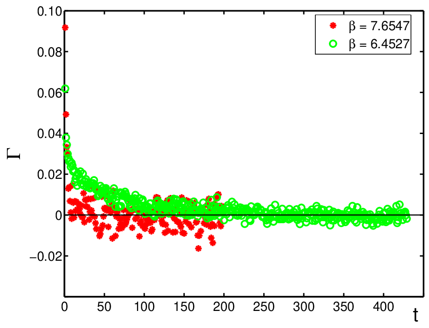
We finally add a remark on error estimates and autocorrelations in our simulations. The autocorrelation function of , defined as in [57], falls very quickly for all our mesurements. At all but the largest coupling the integrated autocorrelation time is then easily estimated. However for , we observe that shows a long tail before approaching zero. This pattern is absent in the smaller volumes, and shows little sensitivity to changes of . Figure 7 (left) plots the -function obtained from runs with , for two different physical volumes. Figure 7 (right) shows that for the integrated autocorrelation time is quite short, i.e. , whereas for the tail mentioned above leads to . The latter translates into an increase of the error by a factor of two, in comparison to the case where no correlation is present (i.e. ).
References
- [1] E. Eichten and B. Hill, An effective field theory for the calculation of matrix elements involving heavy quarks, Phys. Lett. B234 (1990) 511.
- [2] B. Grinstein, The static quark effective theory, Nucl. Phys. B339 (1990) 253–268.
- [3] H. Georgi, An effective field theory for heavy quarks at low energies, Phys. Lett. B240 (1990) 447–450.
- [4] M. Bochicchio, G. Martinelli, C. R. Allton, C. T. Sachrajda, and D. B. Carpenter, Heavy quark spectroscopy on the lattice, Nucl. Phys. B372 (1992) 403–420.
- [5] V. Gimenez, G. Martinelli, and C. T. Sachrajda, A high-statistics lattice calculation of and in the B-meson, Nucl. Phys. B486 (1997) 227–244, [hep-lat/9607055].
- [6] JLQCD Collaboration, S. Aoki et. al., Heavy quark expansion parameters from lattice nrqcd, Phys. Rev. D69 (2004) 094512, [hep-lat/0305024].
- [7] E. Eichten and B. Hill, Static effective field theory: corrections, Phys. Lett. B243 (1990) 427–431.
- [8] J. M. Flynn and B. R. Hill, B - B∗ splitting: A test of heavy quark methods, Phys. Lett. B264 (1991) 173–177.
- [9] M. Lüscher, P. Weisz, and U. Wolff, A numerical method to compute the running coupling in asymptotically free theories, Nucl. Phys. B359 (1991) 221–243.
- [10] ALPHA Collaboration, A. Bode et. al., First results on the running coupling in QCD with two massless flavors, Phys. Lett. B515 (2001) 49–56, [hep-lat/0105003].
- [11] ALPHA Collaboration, S. Capitani, M. Lüscher, R. Sommer, and H. Wittig, Non-perturbative quark mass renormalization in quenched lattice QCD, Nucl. Phys. B544 (1999) 669, [hep-lat/9810063].
- [12] ALPHA Collaboration, J. Heitger and R. Sommer, Non-perturbative heavy quark effective theory, JHEP 02 (2004) 022, [hep-lat/0310035].
- [13] M. Della Morte, N. Garron, M. Papinutto, and R. Sommer, Heavy quark effective theory computation of the mass of the bottom quark, JHEP 01 (2007) 007, [hep-ph/0609294].
- [14] J. H. Kuhn, M. Steinhauser, and C. Sturm, Heavy quark masses from sum rules in four-loop approximation, hep-ph/0702103.
- [15] ALPHA Collaboration, J. Rolf and S. Sint, A precise determination of the charm quark’s mass in quenched QCD, JHEP 12 (2002) 007, [hep-ph/0209255].
- [16] D. Guazzini, R. Sommer, and N. Tantalo, and from a combination of hqet and qcd, PoS LAT2006 (2006) 084, [hep-lat/0609065].
- [17] ALPHA Collaboration, M. Kurth and R. Sommer, Renormalization and O()-improvement of the static axial current, Nucl. Phys. B597 (2001) 488–518, [hep-lat/0007002].
- [18] M. Della Morte, A. Shindler, and R. Sommer, On lattice actions for static quarks, JHEP 08 (2005) 051, [hep-lat/0506008].
- [19] ALPHA Collaboration, M. Della Morte et. al., Lattice hqet with exponentially improved statistical precision, Phys. Lett. B581 (2004) 93–98, [hep-lat/0307021].
- [20] M. Lüscher, S. Sint, R. Sommer, and P. Weisz, Chiral symmetry and O() improvement in lattice QCD, Nucl. Phys. B478 (1996) 365–400, [hep-lat/9605038].
- [21] ALPHA Collaboration, J. Heitger, A. Jüttner, R. Sommer, and J. Wennekers, Non-perturbative tests of heavy quark effective theory, JHEP 11 (2004) 048, [hep-ph/0407227].
- [22] R. Sommer, Non-perturbative qcd: Renormalization, o-improvement and matching to heavy quark effective theory, hep-lat/0611020.
- [23] A. F. Falk, B. Grinstein, and M. E. Luke, Leading mass corrections to the heavy quark effective theory, Nucl. Phys. B357 (1991) 185–207.
- [24] G. Amoros, M. Beneke, and M. Neubert, Two-loop anomalous dimension of the chromo-magnetic moment of a heavy quark, Phys. Lett. B401 (1997) 81–90, [hep-ph/9701375].
- [25] A. Czarnecki and A. G. Grozin, Hqet chromomagnetic interaction at two loops, Phys. Lett. B405 (1997) 142–149, [hep-ph/9701415].
- [26] A. Grozin, P. Marquard, J. Piclum, and M. Steinhauser SFB/TR 09, to be published.
- [27] M. Lüscher, R. Sommer, P. Weisz, and U. Wolff, A precise determination of the running coupling in the SU(3) Yang-Mills theory, Nucl. Phys. B413 (1994) 481–502, [hep-lat/9309005].
- [28] E. Eichten and F. Feinberg, Spin dependent forces in qcd, Phys. Rev. D23 (1981) 2724.
- [29] D. Gromes, Spin dependent potentials in qcd and the correct long range spin orbit term, Z. Phys. C26 (1984) 401.
- [30] N. Brambilla, A. Pineda, J. Soto, and A. Vairo, Effective field theories for heavy quarkonium, hep-ph/0410047.
- [31] Y. Koma and M. Koma, Spin-dependent potentials from lattice qcd, hep-lat/0609078.
- [32] E. Eichten and B. Hill, Renormalization of heavy - light bilinears and for Wilson fermions, Phys. Lett. B240 (1990) 193.
- [33] M. Della Morte, R. Hoffmann, and F. Knechtli, Discrete symmetries of lattice qcd (and the sf), Internal notes of the ALPHA Collaboration (2005).
- [34] S. Sint and R. Sommer, The running coupling from the QCD Schrödinger functional: A one loop analysis, Nucl. Phys. B465 (1996) 71–98, [hep-lat/9508012].
- [35] ALPHA Collaboration, S. Sint and P. Weisz, The running quark mass in the sf scheme and its two loop anomalous dimension, Nucl. Phys. B545 (1999) 529, [hep-lat/9808013].
- [36] ALPHA Collaboration, M. Della Morte et. al., Non-perturbative quark mass renormalization in two-flavor qcd, Nucl. Phys. B729 (2005) 117–134, [hep-lat/0507035].
- [37] ALPHA Collaboration, M. Guagnelli, R. Sommer, and H. Wittig, Precision computation of a low-energy reference scale in quenched lattice QCD, Nucl. Phys. B535 (1998) 389, [hep-lat/9806005].
- [38] A. Huntley and C. Michael, Spin spin and spin - orbit potentials from lattice gauge theory, Nucl. Phys. B286 (1987) 211.
- [39] ALPHA Collaboration, M. Guagnelli, J. Heitger, C. Pena, S. Sint, and A. Vladikas, Non-perturbative renormalization of left-left four-fermion operators in quenched lattice qcd, JHEP 03 (2006) 088, [hep-lat/0505002].
- [40] F. Palombi, C. Pena, and S. Sint, A perturbative study of two four-quark operators in finite volume renormalization schemes, JHEP 03 (2006) 089, [hep-lat/0505003].
- [41] F. Palombi, M. Papinutto, C. Pena, and H. Wittig, A strategy for implementing non-perturbative renormalisation of heavy-light four-quark operators in the static approximation, JHEP 08 (2006) 017, [hep-lat/0604014].
- [42] C. Pena, Twisted mass qcd for weak matrix elements, PoS LAT2006 (2006) 019, [hep-lat/0610109].
- [43] ALPHA Collaboration, J. Heitger, M. Kurth, and R. Sommer, Non-perturbative renormalization of the static axial current in quenched qcd, Nucl. Phys. B669 (2003) 173–206, [hep-lat/0302019].
- [44] M. Della Morte, P. Fritzsch, and J. Heitger, Non-perturbative renormalization of the static axial current in two-flavour qcd, JHEP 02 (2007) 079, [hep-lat/0611036].
- [45] S. Kurth, The renormalised quark mass in the Schrödinger functional of lattice QCD: A one-loop calculation with a non- vanishing background field, hep-lat/0211011.
- [46] R. Narayanan and U. Wolff, Two loop computation of a running coupling in lattice yang- mills theory, Nucl. Phys. B444 (1995) 425–446, [hep-lat/9502021].
- [47] ALPHA Collaboration, A. Bode, P. Weisz, and U. Wolff, Two loop computation of the Schrödinger functional in lattice QCD, Nucl. Phys. B576 (2000) 517–539, [Erratum-ibid.B600:453,2001, Erratum-ibid.B608:481,2001, hep-lat/9911018].
- [48] P. Weisz, Computation of the improvement coefficient to 1-loop, Internal notes of the ALPHA Collaboration (1996).
- [49] M. Creutz, Quarks, gluons and lattices, . Cambridge, Uk: Univ. Pr. ( 1983) 169 P. ( Cambridge Monographs On Mathematical Physics).
- [50] G. M. de Divitiis, R. Frezzotti, M. Guagnelli, and R. Petronzio, Nonperturbative determination of the running coupling constant in quenched su(2), Nucl. Phys. B433 (1995) 390–402, [hep-lat/9407028].
- [51] N. Cabibbo and E. Marinari, A new method for updating su(n) matrices in computer simulations of gauge theories, Phys. Lett. B119 (1982) 387–390.
- [52] K. Fabricius and O. Haan, Heat bath method for the twisted eguchi-kawai model, Phys. Lett. B143 (1984) 459.
- [53] A. D. Kennedy and B. J. Pendleton, Improved heat bath method for monte carlo calculations in lattice gauge theories, Phys. Lett. B156 (1985) 393–399.
- [54] M. Creutz, Overrelaxation and monte carlo simulation, Phys. Rev. D36 (1987) 515.
- [55] G. Parisi, R. Petronzio, and F. Rapuano, A measurement of the string tension near the continuum limit, Phys. Lett. 128B (1983) 418.
- [56] M. Lüscher and P. Weisz, Locality and exponential error reduction in numerical lattice gauge theory, JHEP 09 (2001) 010, [hep-lat/0108014].
- [57] ALPHA Collaboration, U. Wolff, Monte carlo errors with less errors, Comput. Phys. Commun. 156 (2004) 143–153, [hep-lat/0306017].