Magnetic focusing of charge carriers from spin-split bands: Semiclassics of a Zitterbewegung effectJournal: New J. Phys.
Abstract
We present a theoretical study of the interplay between cyclotron motion and spin splitting of charge carriers in solids. While many of our results apply more generally, we focus especially on the Rashba model describing electrons in the conduction band of asymmetric semiconductor heterostructures. Appropriate semiclassical limits are distinguished that describe various situations of experimental interest. Our analytical fomulae, which take full account of Zeeman splitting, are used to analyse recent magnetic-focusing data. Surprisingly, it turns out that the Rashba effect can dominate the splitting of cyclotron orbits even when the Rashba and Zeeman spin-splitting energies are of the same order. We also find that the origin of spin-dependent cyclotron motion can be traced back to Zitterbewegung-like oscillatory dynamics of charge carriers from spin-split bands. The relation between the two phenomena is discussed, and we estimate the effect of Zitterbewegung-related corrections to the charge carriers’ canonical position.
pacs
72.25.Dc, 03.65.Sq, 73.23.Ad, 71.70.Ej1 Introduction
Magnetic focusing of ballistic charge carriers in metals [1, 2] and semiconductors [3, 4, 5] has been successfully used to elucidate fundamental materials properties such as the shape of the Fermi surface [6, 7], Andreev reflection in superconductor/normal-metal hybrid structures [8, 9], surface crystallography [10], phase coherent transport [3], and emergent quasiparticles in the fractional-quantum-Hall regime [11]. The fundamental setup of a magnetic-focusing experiment is quite simple; see Figure 1.

It requires sufficiently ballistic transport between two fixed, co-linear (injector and collector) contacts. A large number of injected-particle trajectories converge at the collector every time the contact separation equals an integer multiple of the cyclotron diameter . Peaks occurring in the measured collector voltage at concomitant magnetic fields are the experimental signature for magnetic focusing. Recently, magnetic-focusing trajectories of electrons in a two-dimensional semiconductor heterostructure have been imaged directly using scanning-probe microscopy [12].
Several experiments [13, 14, 15, 16, 17] have investigated the possibility to spatially separate charge carriers belonging to spin-split bands using the magnetic-focusing technique, which may have ramifications for the emerging field of spin electronics [18, 19]. The desire to use magnetic-field-independent, spin-orbit-induced spin splitting for this purpose [14, 15, 16, 17] is fuelling renewed interest [20, 21, 22, 23, 24] in the theoretical study of spin-orbit effects in the semiclassical regime [25, 26, 27, 28, 29, 30, 31, 32, 33, 34, 35, 36, 37]. We present a critical analysis of the interplay between spin-orbit coupling and cyclotron motion in both quantum and semiclassical regimes, with particular emphasis on spin-dependent magnetic focusing. We also discuss this effect in the context of another topic of great current interest, namely Zitterbewegung in solid-state systems [38, 39, 40, 41, 42, 43, 44], and comment on the (un-)suitability of proposed intuitive interpretations in terms of a spin-dependent focusing field [14] or a spin-dependent Lorentz force [45, 46, 47].
This article is organised as follows. We start by reviewing semiclassical theories that have been developed for systems with finite spin splitting. These theoretical approaches are then applied to describe cyclotron motion of charge carriers in two-dimensional (2D) heterostructures subject to both Zeeman and Rashba [48, 49] spin splittings. Our results are used to analyse recent experimental data obtained from p-type GaAs [14] and n-type InSb [16, 17] samples. Subsequently, we discuss the intricate connection between spin-dependent magnetic focusing and Zitterbewegung of charge carriers from spin-split bands [39, 40, 41, 43]. Conclusions are given in the final Section.
2 Basic aspects of semiclassics in presence of spin splitting
Non-relativistic single-particle Hamiltonians with spin splitting can generally be written in the form [32, 33, 34, 35, 36]
| (1) |
Here we denote the particle’s position, momentum, and spin angular-momentum operators by , , and , respectively, where is the vector of generators for SU(2) rotations in the spin- representation, and is the Planck constant. The vector operator represents an effective magnetic field that contains, in general, contributions due to the Zeeman effect and spin-orbit coupling. Note that has the dimensionality 1/time. In the following, we distinguish three possible semiclassical limits. To keep our notation uncluttered, we do not explicitly distinguish quantum-mechanical operators from their associated semiclassical phase-space symbols. We will clearly separate the discussion of purely quantum and semiclassical properties to avoid any possible confusion arising from this simplification.
2.1 Precessing-spin semiclassics
Representing a truly quantum-mechanical correction, the second (spin-splitting) term in (1) vanishes in the usual semiclassical limit that is defined as such that remains constant. As a result, the semiclassical orbital dynamics is unaffected by the spin degree of freedom [31, 32, 33]. The classical trajectory , as determined by , prescribes the dynamics of the classical spin via a precession-type equation of motion
| (2) |
i.e., we can interpret as the precession frequency. This type of semiclassics has also been called a weak-coupling limit [32, 33, 34, 35, 36]. Physically, it corresponds to the regime of a perfectly classical, spin-independent orbital motion with an associated trajectory-dependent precession of a classical spin [31, 32, 33, 34].
In many experimentally relevant situations the appropriate semiclassical description will be of the precessional type discussed here. This has, e.g., been shown for anomalous magneto-oscillations [37]. However, there are experimentally accessible regimes where the spin dynamics actually influences the orbital motion. Spin-dependent cyclotron motion represents a pertinent example [14, 16, 17]. The semiclassical description of such situations is desirable, motivating the consideration of alternative schemes for performing the classical limit. We proceed to discuss two of these, both of which correspond to a strong-coupling-type semiclassics.
2.2 Spin-orbit-intertwined semiclassics
One possibility to keep the spin-splitting term in the Hamiltonian (1) finite in the semiclassical limit is to simultaneously require to remain constant, which implies . The time evolution of the spin state will then affect orbital dynamics and vice versa. The resulting set of semiclassical equations of motion is given by [33]
| (3a) | |||||
| (3b) | |||||
| (3c) | |||||
Hence, in this case, the spin and orbital dynamics are mutually affecting each other. These equations of motion have previously occured in [35, 36], but without noticing that they only provide the leading semiclassical dynamics when is considered in addition to . Moreover, in [35, 36] the notion of an extended phase space was introduced, intending to stress the role of spin as an independent classical dynamical variable. Kinematically, the same phase space arises in the precessing-spin semiclassics; however, in that context the spin-orbit dynamics are not of a Hamiltonian form because the spin dynamics is driven by the orbital motion, without any feedback of the spin dynamics on the orbital motion.
2.3 Adiabatic-spin semiclassics
An alternative, in some sense very-strong-coupling [25, 26, 27, 32, 34, 36] semiclassics is obtained by letting while keeping the spin projection frozen to a quantised value with respect to the instantaneous direction of . Then the associated orbital dynamics is governed by the Hamiltonian
| (3d) |
For each possible value , ranging over , a generally different classical trajectory is obtained. In contrast to the two cases discussed above, here the spin degree of freedom itself has no dynamics; it just introduces a Berry-phase-like contribution to the orbital motion [50]. To avoid the problem of mode-conversion, this approach is restricted to the case for every point along a trajectory [25, 26].
3 Application to the Landau-Rashba model
To be specific, we consider the Landau-Rashba model [49, 48] that describes spin conduction-band electrons in an asymmetric 2D heterostructure subject to a perpendicular magnetic field . It is of the form given in (1), with
| (3ea) | |||||
| (3eb) | |||||
Here and are the effective mass and Landé factor of the 2D electrons, with the electron mass in vacuum, and characterises the strength of the Rashba spin splitting [49, 48]. The 2D heterostructure growth direction is taken as the Cartesian axis; with being the associated unit vector.
3.1 Quantum solution: Jaynes-Cummings model
A complete quantum solution of the Landau-Rashba model is available [51], as it is equivalent [36] to the exactly soluble Jaynes-Cummings (JC) model [52] in the rotating-wave approximation. (The JC model describes coupling of a harmonic oscillator, here associated with the Landau levels, to a two-level system, here represented by the electronic spin degree of freedom.) Using techniques developed in theoretical quantum optics [53], we recently obtained [43] the exact Heisenberg time evolution of spin and position operators. The perpendicular-to-the-plane spin component can be separated into two parts, , with time-independent and oscillating parts given by
| (3efa) | |||||
| (3efb) | |||||
Here is an effective magnetic-field operator that governs spin precession in the Landau-Rashba model. Similarly, the 2D position operator can be decomposed into a constant part, which corresponds to the guiding-centre position of a cyclotron orbit, and a time-dependent oscillatory part. For the sake of brevity, we will use a compact complex notation [54] for 2D position and kinetic-momentum : , , and extend this notation also to the in-plane spin components: . In the Heisenberg picture, the time evolution of the complex 2D position is then given by , with
| (3efga) | |||||
Here , and is the cyclotron frequency of electrons in the semiconductor material.
In principle, the expressions given in (3efa)-(3efg) allow for the calculation of time-dependent spin and position expectation values for any initial state. In practice, such a calculation may turn out to be rather cumbersome and difficult to interpret. Hence, in the following, we will discuss magnetic focusing in the context of semiclassical approaches applied to the Landau-Rashba model. Approximate semiclassical approaches are often practical for understanding certain physical phenomena and also provide a rather general framework to treat quantum systems of interest. However, the above exact results provide a useful benchmark for their reliability.
3.2 Precessing-spin semiclassics of the Landau-Rashba model
In this case, the orbital dynamics is entirely governed by the Landau model. Using the compact complex notation introduced above, we have
| (3efgha) | |||||
| (3efghb) | |||||
The spin dynamics is determined by the precession equation (2), where is given by (3eb). For the and in-plane components and , they read explicitly
| (3efghia) | |||||
| (3efghib) | |||||
[The equation for follows from complex conjugation of (3efghia).] From (3efghia) and (3efghib), it follows that
| (3efghija) | |||
| with the spin-precession-related frequency scale | |||
| (3efghijb) | |||
Note that . Integration yields
| (3efghijka) | |||||
| (3efghijkb) | |||||
with arbitrary constants . Inserting this result into (3efghia) enables one to find . We omit this step here.
It is illustrating to note that emerges as the eigenvalue of the JC Hamiltonian in the limit where the kinetic-momentum operators and are treated as -numbers. This corresponds to the early semiclassical treatments of the JC model [55]. Thus (3efghijkb) with (3efghijb) reflects the exact quantum solution for spin precession in the Landau-Rashba model (3efb) taken in the appropriate weak-coupling limit. Our results obtained here generalise those presented in Sec. 5.1.1 of Ref. [36] where the weak-coupling limit of the Landau-Rashba model was previously discussed. The complete disappearance of from the dynamics described in this Section is an expected feature of the precessing-spin semiclassical limit.
3.3 Adiabatic-spin semiclassics of the Landau-Rashba model
In the limit where the electron spin is assumed to be either aligned or anti-aligned with the local field [given by (3eb)], the Landau-Rashba model specialises to a pair of terms of the form (3d) that govern the dynamics of electrons with spin projection . As the Rashba and Zeeman contributions to are perpendicular to each other, we have
| (3efghijkl) |
Thus is again a constant of the motion. For a fixed value of conserved energy , it assumes two different values for particles distinguished by spin projection , where . The values of can be found from
| (3efghijkm) |
The equations of motion resulting from Hamiltonians (3d) for the Landau-Rashba case can be written as
| (3efghijkna) | |||||
| (3efghijknb) | |||||
| which describe cyclotron motion with a spin-dependent effective mass | |||||
| (3efghijknc) | |||||
and thus spin-dependent frequency . The cyclotron radius is different for the two spin species because of their different values of for fixed energy . A straightforward calculation yields
| (3efghijkno) |
A few comments about our results are in order. Firstly, the fact that the above expressions for spin-dependent cyclotron frequency and radius depend on the parameter (which has the dimension of velocity) is a direct consequence of the way the adiabatic-spin semiclassical limit is performed. Secondly, for , our expression for is exactly the same as that found in Ref. [21] where, ostensibly, the spin-orbit-intertwined semiclassical limit was discussed. Also, our result for agrees with the corresponding expression from Ref. [21] to leading order in the large- limit. Apparently, the approximate scheme employed by the authors of Ref. [21] is essentially equivalent to the adiabatic-spin semiclassics, even though they recover a finite component of spin as given in Equation (3efa) above. Thus a consistent treatment of the Landau-Rashba model using spin-orbit-intertwined semiclassics seems to be still lacking. Thirdly, the canonical equations of motion (3efghijkna) and (3efghijknb) indicate that the effect of adiabatic-spin semiclassics on the orbital dynamics is better described as a renormalisation of the effective mass [48, 22] than a renormalisation of the focusing field [14]. Lastly, (3efghijknb) represents the familiar expression of the Lorentz force in terms of a particle’s velocity without any trace of the previously claimed [46] spin-dependent contribution. Such a result is expected from proper quantum-mechanical derivations [56] of the Lorentz-force operator.
3.4 Analysis of magnetic-focusing experiments
To leading order, no spin splitting of magnetic-focusing peaks occurs in the precessing-spin semiclassical limit. For this case, back action of spin dynamics on orbital motion may appear only in corrections of order that can be included in principle [57]. Instead of considering this possibility, we focus here on the adiabatic-spin semiclassics which provides a proper description of magnetic focusing already in leading order.
It is useful to define effective wave-vector scales and , which are associated with the 2D carrier sheet density and Rashba spin splitting, respectively. After equating from (3efghijkno) with the contact separation and performing some straightforward algebra, we find a relation that has to be satisfied by each of the two experimentally observed focusing fields :
| (3efghijknp) |
Thus measurement of the spin-split focusing peaks allows to determine both and directly, with the effective electron mass entering only the parameter . For , the relation (3efghijknp) specialises to , which was used in Ref. [14] to extract in a GaAs 2D hole system. Table 1 summarises values obtained from existing magnetic-focusing data, taking into account the finite Zeeman splitting. It turns out that, for the sample parameters realised in these experiments, the dependence of extracted on is rather weak over an extended range before Zeeman splitting becomes suddenly dominant. This surprising feature, which is illustrated in Figure 2, explains why it was possible to extract a reasonable value for in Ref. [14] even though, in that experiment, Rashba and Zeeman spin splittings were of comparable magnitude for states at the Fermi energy. Note, however, that the range of parameter over which Rashba splitting can be reliably extracted will be reduced in samples with smaller contact separation and concomitantly higher focusing fields.
| material | [nm] | [nm-1] | [T] | [T] | [nm-1] | [nm-1] | |
|---|---|---|---|---|---|---|---|
| p-GaAs† | 1.4 | 800 | 0.093 | 0.17 | 0.20 | 0.11 | 0.009 |
| n-InSb‡ | 0.36 | 600 | 0.14 | 0.30 | 0.36 | 0.15 | 0.014 |
| n-InSb∗ | 0.36 | 600 | 0.19 | 0.37 | 0.50 | 0.20 | 0.030 |
† From Ref. [14]. As in this work, we apply the -linear Rashba model for conduction-band electrons to interpret the data. A more detailed study would have to take into account fundamental differences between Rashba spin splitting in 2D electron and hole systems [58].
‡ From Ref. [16].
∗ From Ref. [17]. The given value of is derived from the focusing field (0.42 T) expected in the absence of spin splitting (as stated by the authors).
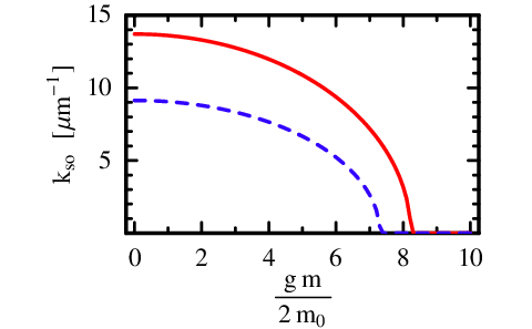
The values of given in Table 1 are on the order of 10% of the effective Fermi wave number . Thus the applicability of the adiabatic-spin semiclassics for typical experimental situations could be questioned. A detailed discussion of this point would benefit from a fuller understanding of spin-orbit-intertwined semiclassics in the Landau-Rashba model, which is currently lacking. Incidentally, results from a numerical simulation [20] performed using experimentally realistic parameters provide strong support for the assumption of adiabatic-spin dynamics.
Our analysis of experimental data focused exclusively on the first magnetic-focusing peak. This allowed us to neglect scattering at the lithographic barrier between injector and collector contacts, which is relevant for higher-order focusing peaks. Within a ballistic semiclassical approach such as ours, spin flips occuring during collision with the sample edge can be taken into account phenomenologically [59] by including the possibility for particles to continue on either one of the spin-split cyclotron orbits after each reflection. This model predicts that the second peak will be unsplit (split into three parts) in the absence (presence) of boundary spin-flip scattering [17].
4 Relation to Zitterbewegung
Zitterbewegung (ZB) was originally introduced by Schrödinger as the technical term for an oscillatory orbital motion performed by free relativistic electrons whose dynamics is governed by the Dirac equation. See Refs. [60, 61, 62, 63] for modern descriptions of the effect. ZB has never been directly observed, partly because the associated period and amplitude ( s and Å, respectively, for electrons in vacuum) are out of reach for any current experimental equipment. For ultra-relativistic particles, the ZB amplitude is of the order of the de Broglie wave length [43], limiting the suitability of scattering experiments to detect the effect.
Analogs of ZB in a nonrelativistic solid-state context have recently attracted great interest [38, 39, 40, 41, 42, 43, 44]. In particular, charge carriers from spin-split bands are expected to perform an oscillatory motion that is entirely analogous to ZB [39, 40, 41, 43]. The experimentally observed [64, 65] zero-field spin precession of electrons and holes turns out to be closely related to ZB [43], but no direct ramification of ZB in coordinate space has been measured. Theoretical studies suggest [66, 41, 43] that ZB results in a spatial separation of carriers with opposite spin that is of the order of the de Broglie wave length. Here we show that spin-dependent magnetic focusing is also closely related with ZB. For the sake of notational simplicity, we neglect Zeeman splitting from now on and consider only the limit of sufficiently small magnetic fields where Landau-quantisation effects are negligible.
4.1 Cyclotron motion of charge carriers performing Zitterbewegung
It is a consequence of ZB that the time-dependent position [velocity, spin] operators [, ] can be written as the sum of an average (smoothened over ZB) part [, ] and an oscillatory part [, ]. Universal expressions, in terms of suitably defined ZB frequency and amplitude operators and , have been obtained for all these operators for a range of (multi-band) models [43]. For example, the average part of the velocity is given by
| (3efghijknq) |
for any two-band Hamiltonian , including the Rashba model. We continue by discussing this special case only. A finite acceleration of the (ostensibly free!) particles performing ZB in zero magnetic field is found
| (3efghijknr) |
where the r.h.s expression is the specialisation to the Rashba-model case, and we used the appropriate expression for that, within our current notation, reads
| (3efghijkns) |
As the r.h.s of (3efghijknr) indicates, this acceleration is intimately related to spin precession in the Rashba model. In particular, the fact that in zero magnetic field is directly associated with the vanishing time average of the ZB-related acceleration (3efghijknr) for this case.
A finite perpendicular magnetic field forces charged particles on cyclotron orbits and, therefore, leads to additional time dependences of their dynamical variables. To elucidate the interplay between ZB and classical cyclotron motion more clearly than it emerges, eg, from the exact solution of the JC model given in Sec. 3.1, we concentrate on the low-field limit where the time scales associated with these two effects are well-separated. This regime allows one to consider quantities that are averaged over the ZB time scale but are still time-dependent because of the cyclotron motion.
As indicated by (3efa), becomes finite in a perpendicular magnetic field. In that situation, the average of the acceleration (3efghijknr) over the ZB time scale becomes finite and yields, in the low-field regime and with Zeeman splitting neglected, the Lorentz-force-like term
| (3efghijknt) |
To obtain (3efghijknt), we used (3efa) above, as well as the relation (3efghijknq) specialised to the Landau-Rashba model in the low-field limit (where the non-commutativity of and can be neglected),
| (3efghijknu) |
The total ZB-averaged acceleration experienced by a charged particle subject to a magnetic field is given, in the low-field limit, by the sum of the ordinary Lorentz-force contribution and the finite ZB-averaged acceleration (3efghijknt). It turns out to have the form
| (3efghijknv) |
ie, is determined by the ZB-averaged velocity derived from (3efghijknu). Applying the adiabatic-spin semiclassical limit, (3efghijknu) specialises to (3efghijkna), and (3efghijknv) is equivalent to (3efghijknb). Hence the spin-dependent cyclotron mass emerges because of the ZB contribution (3efghijknt) to the total acceleration (3efghijknv). Similar to the spatial separation of spin-polarised partial waves for an unpolarised electron beam injected into a wave guide [66], spin-dependent cyclotron motion is thus a direct consequence of ZB-related dynamics arising in the presence of spin splitting.
As noted already a long time ago [61], ZB-related terms can contribute to expectation values of observables such as . Similarly, the evaluation of for eigenstates of the Landau-Rashba model at fixed energy yields a hint of the existence of two different cyclotron orbits for electrons from spin-split bands [21].
4.2 Corrections due to anomalous position operator
The effective Rashba Hamiltonian describing electrons in the conduction band can be thought of as arising from a canonical transformation (Löwdin partitioning [58]) that is similar to the Foldy-Wouthuysen transformation [67] needed to arrive at the proper non-relativistic limit of Dirac-electron theory. That same transformation will change the form of the physical position operator associated with a point-like particle, which will then be different from the canonical position operator acting in the reduced Hilbert space of the conduction band. For Dirac electrons, the two position operators have been proposed to be associated with a particle’s centre of charge and centre of mass, respectively [61]. See Ref. [68] for a closely related discussion refering to solid state systems. Transport measurements such as the ones employed by the magnetic-focusing technique can be expected to be sensitive to the physical (charge) position rather than the canonical (mass) one.
The formal relation between physical position and the canonical one is
| (3efghijknw) |
where is the (effective) Compton wave length. Typical -values for carriers in generic semiconductors can be found in Refs. [38, 43]. In a finite magnetic field, the shift between physical and canonical position gives rise to a correction to spin-split cyclotron radii that is of the order of and, therefore, usually quite small. A possible exception could be InSb where nm.
5 Conclusions
We have studied theoretically the cyclotron motion of charge carriers from spin-split bands, highlighting exact quantum and semiclassical results for electrons in asymmetric 2D semiconductor heterostructures. A spin-dependent splitting of cyclotron orbits is found in the adiabatic-spin semiclassical limit. Relevant parameters of real samples used in recent magnetic-focusing experiments were extracted, taking full account of Zeeman splitting. Our analytical formulae should also be useful for analysis and design of future spin-dependent focusing measurements. We furthermore elucidated the intricate relationship between spin-split cyclotron orbits and Zitterbewegung of charge carriers in systems with strong spin-orbit coupling.
Acknowledgments
RW and UZ received support from the National Science Foundation under Grant No. PHY99-07949 while visiting the Kavli Institute for Theoretical Physics (University of California, Santa Barbara, USA) where part of this work was performed. The authors thank R Danneau, A R Hamilton, J J Heremans, A P Micolich, J Sinova, and G Vignale for illuminating discussions.
References
References
- [1] Sharvin Yu V and Fisher L M 1965 Pis’ma Zh. Eksp. Teor. Fiz. 1 58 [JETP Lett. 1 152]
- [2] Tsoi V S 1974 Pis’ma Zh. Eksp. Teor. Fiz. 19 114 [JETP Lett. 19 70]
- [3] van Houten H, Beenakker C W J, Williamson J G, Broekaart M E I, van Loosdrecht P H M, van Wees B J, Mooij J E, Foxon C T, and Harris J J 1989 Phys. Rev. B 39 8556
- [4] Beenakker C W J and van Houten H in Ehrenreich H and Turnbull D (ed) 1991 Solid State Physics volume 44 (San Diego: Academic Press) pp 1–228. See, in particular, pp. 125–135 and references cited therein.
- [5] Heremans J J, Santos M B, and Shayegan M 1992 Appl. Phys. Lett. 61 1652
- [6] Tsoi V S, Bass J, Benistant P A M, van Kempen H, Payens E L M, and Wyder P 1979 J. Phys. F 9 L221
- [7] Heremans J J, Santos M B, and Shayegan M 1994 Surf. Sci. 305 348
- [8] Bozhko S I, Tsoi V S, and Yakovlev S E 1982 Pis’ma Zh. Eksp. Teor. Fiz. 36 123 [JETP Lett. 36 153]
- [9] Benistant P A M, van Kempen H, and Wyder P 1983 Phys. Rev. Lett. 51 817
- [10] Tsoi V S, Bass J, and Wyder P 1999 Rev. Mod. Phys. 71 1641
- [11] Goldman V J, Su B, and Jain J K 1994 Phys. Rev. Lett. 72 2065
- [12] Aidala K E, Parrott R E, Kramer T, Heller E J, Westervelt R M, Hanson M P, and Gossard A C 2007 Nature Phys. 3 464
- [13] Potok R M, Folk J A, Marcus C M, and Umansky V 2002 Phys. Rev. Lett. 89 266602
- [14] Rokhinson L P, Larkina V, Lyanda-Geller Yu B, Pfeiffer L N, and West K W 2004 Phys. Rev. Lett. 93 146601
- [15] Rokhinson L P, Pfeiffer L N, and West K W 2006 Phys. Rev. Lett. 96 156602
- [16] Dedigama A R, Deen D, Murphy S Q, Goel N, Keay J C, Santos M B, Suzuki K, Miyashita S, and Hirayama Y 2006 Physica E 34 647
- [17] Heremans J J, Chen H, Santos M B, Goel N, Van Roy W, and Borghs G 2007 AIP Conf. Proc. 893 1287
- [18] Wolf S A, Awschalom D D, Buhrmann R A, Daughton J M, von Molnár S, Roukes M L, Chtchelkanova A Y, and Treger D M 2001 Science 294 1488
- [19] Zutić I, Fabian J, and Das Sarma S 2004 Rev. Mod. Phys. 76 323
- [20] Usaj G and Balseiro C A 2004 Phys. Rev. B 70 041301(R)
- [21] Reynoso A, Usaj G, Sanchez M J, and Balseiro C A 2004 Phys. Rev. B 70 235344
- [22] Valin-Rodriguez M and Nazmitdinov R G 2006 Phys. Rev. B 73 235306
- [23] Reynoso A, Usaj G, and Balseiro C A 2007 Phys. Rev. B 75 085321
- [24] Reynoso A A, Usaj G, and Balseiro C A 2007 arxiv:cond-mat/0703267
- [25] Littlejohn R G and Flynn W G 1991 Phys. Rev. A 44 5239
- [26] Littlejohn R G and Flynn W G 1992 Phys. Rev. A 45 7697
- [27] Frisk H and Guhr T 1993 Ann. Phys. (NY) 221 229
- [28] Lu J P, Yau J B, Shukla S P, Shayegan M, Wissinger L, Rössler U, and Winkler R 1998 Phys. Rev. Lett. 81 1282
- [29] Lu J P, Shayegan M, Wissinger L, Rössler U, and Winkler R 1999 Phys. Rev. B 60 13776
- [30] Zitzlsperger M, Onderka R, Suhrke M, Rössler U, Weiss D, Wegscheider W, Bichler M, Winkler R, Hirayama Y, and Muraki K 2003 Europhys. Lett. 61 382
- [31] Bolte J and Keppeler S 1998 Phys. Rev. Lett. 81 1987
- [32] Bolte J and Keppeler S 1999 Ann. Phys. (NY) 274 125
- [33] Bolte J and Glaser R 2005 Ann. Henri Poincare 6 625
- [34] Amann C and Brack M 2002 J. Phys. A: Math. Gen. 35 6009
- [35] Pletyukhov M, Amann C, Mehta M, and Brack M 2002 Phys. Rev. Lett. 89 116601
- [36] Pletyukhov M and Zaitsev O 2003 J. Phys. A: Math. Gen. 36 5181
- [37] Keppeler S and Winkler R 2002 Phys. Rev. Lett. 88 046401
- [38] Zawadzki W 2005 Phys. Rev. B 72 085217
- [39] Schliemann J, Loss D, and Westervelt R M 2005 Phys. Rev. Lett. 94 206801
- [40] Schliemann J, Loss D, and Westervelt R M 2006 Phys. Rev. B 73 085323
- [41] Cserti J and Dávid G 2006 Phys. Rev. B 74 172305
- [42] Zawadzki W 2006 Phys. Rev. B 74 205439
- [43] Winkler R, Zülicke U, and Bolte J 2007 Phys. Rev. B 75 205314
- [44] Rusin T M and Zawadzki W 2007 J. Phys.: Condens. Matter 19 136219
- [45] Nikolic B K, Zarbo L P, and Welack S 2005 Phys. Rev. B 72 075335
- [46] Shen S Q 2005 Phys. Rev. Lett. 95 187203
- [47] Zhou B, Ren L, and Shen S Q 2006 Phys. Rev. B 73 165303
- [48] Bychkov Yu A and Rashba E I 1984 Pis’ma Zh. Éksp. Teor. Fiz. 39 66 [JETP Lett. 39 78]
- [49] Bychkov Yu A and Rashba E I 1984 J. Phys. C 17 6039
- [50] Aronov A G and Lyanda-Geller Yu B 1993 Phys. Rev. Lett. 70 343
- [51] Rashba E I 1960 Fiz. Tverd. Tela (Leningrad) 2 1224 [Sov. Phys. Solid State 2 1109]
- [52] Shore B W and Knight P L 1993 J. Mod. Opt. 40 1195
- [53] Barnett S M and Radmore P M 1997 Methods in Theoretical Quantum Optics (Oxford: Clarendon Press)
- [54] MacDonald A H in Akkermans E, Montambaux G, Pichard J L, and Zinn-Justin J (ed) 1995 Mesoscopic Quantum Physics (Amsterdam:Elsevier) pp 659–720
- [55] von Foerster T 1975 J. Phys. A: Math. Gen. 8 95
- [56] Zawadzki W 2007 arxiv:cond-mat/0701378
- [57] Teufel S 2003 Adiabatic Perturbation Theory in Quantum Dynamics, volume 1821 of Lecture Notes in Mathematics (Berlin: Springer)
- [58] Winkler R 2003 Spin-Orbit Coupling Effects in Two-Dimensional Electron and Hole Systems, volume 191 of Springer Tracts in Modern Physics (Berlin: Springer)
- [59] Chen H, Heremans J J, Peters J A, Govorov A O, Goel N, Chung S J, and Santos M B 2005 Appl. Phys. Lett. 86 032113
- [60] Huang K 1952 Am. J. Phys. 20 479
- [61] Barut A O and Bracken A J 1981 Phys. Rev. D 23 2454
- [62] Barut A O and Thacker W 1985 Phys. Rev. D 31 1386
- [63] Thaller B 1992 The Dirac Equation (Berlin: Springer)
- [64] Crooker S A and Smith D L 2005 Phys. Rev. Lett. 94 236601
- [65] Kato Y K, Myers R C, Gossard A C, and Awschalom D D 2005 Appl. Phys. Lett. 87 022503
- [66] Brusheim P and Xu H Q 2006 Phys. Rev. B 74 205307
- [67] Foldy L L and Wouthuysen S A 1950 Phys. Rev. 78 29
- [68] Nozières P and Lewiner C 1973 J. Phys. (Paris) 34 901
- [69] Barut A O and Bracken A J 1982 Aust. J. Phys. 35 353
- [70] Luttinger J 1956 Phys. Rev. 102 1030