A Class of LDPC Erasure Distributions with Closed-Form Threshold Expression
Abstract
In this paper, a family of low-density parity-check (LDPC) degree distributions, whose decoding threshold on the binary erasure channel (BEC) admits a simple closed form, is presented. These degree distributions are a subset of the check regular distributions (i.e. all the check nodes have the same degree), and are referred to as -positive distributions. It is given proof that the threshold for a -positive distribution is simply expressed by . Besides this closed form threshold expression, the -positive distributions exhibit three additional properties. First, for given code rate, check degree and maximum variable degree, they are in some cases characterized by a threshold which is extremely close to that of the best known check regular distributions, under the same set of constraints. Second, the threshold optimization problem within the -positive class can be solved in some cases with analytic methods, without using any numerical optimization tool. Third, these distributions can achieve the BEC capacity. The last property is shown by proving that the well-known binomial degree distributions belong to the -positive family.
I Introduction
The unavailability of a closed form expression for the decoding threshold of low-density parity-check (LDPC) codes still represents an open problem. So far, no general closed form threshold expression is known for any transmission channel. Some results in this sense have been developed for the binary erasure channel (BEC), for which some analytic threshold expressions have been proposed. In [1], an analytic threshold expression has been presented for regular LDPC ensembles. A more general analytic expression, valid for check regular ensembles, has been proposed in [2]. To the best of the authors’ knowledge, the most general analytic expression currently available is that one developed in [3], which can be applied to fully irregular ensembles. For regular or check regular ensembles, the formula proposed in [3] coincides with that one from [2]. The problem with these expressions is that none of them can be really considered a closed form one (except for the case of regular LDPC ensembles with degree-2 variable nodes presented in [1]). In fact, in all these formulas, the threshold is a function of some parameter which in general does not admit a closed form expression. This parameter, which depends on the degree distribution, can be a root of a real polynomial, a fixed point of a real function, or the abscissa of the tangent point between two EXIT curves [4].
An exception is represented by the degree distributions for which the first occurrence of a tangency point between the EXIT curves in the EXIT chart appears for a value of the a priori mutual information equal to 1 (this is sometimes referred to as derivative matching condition). Denoting the decoding threshold by , these distributions achieve with equality the stability condition [5] (which holds for any distribution). This paper presents a family of check regular LDPC distributions, called -positive distributions, which are a subset of the distributions achieving the derivative matching condition. The starting point for obtaining this family is the afore mentioned analytic formula developed in [2].
The name “-positive” is chosen because these distributions are defined as those ones for which a certain polynomial , whose coefficients depend on the edge-oriented variable distribution and on the degree of the check nodes, is non-negative between 0 and 1. The theory of polynomials can be applied to obtain conditions for a check regular distribution to be -positive. A useful theorem in this sense is the Fourier-Budan theorem [6, p. 27], which states an upper bound to the number of real roots in a given interval, for a polynomial with real coefficients. The application of the Fourier-Budan theorem to the polynomial leads to a set of inequalities involving the coefficients ’s and , which represent a necessary condition for a distribution to be -positive.
Besides the closed form threshold expression, the -positive distributions are shown to exhibit some additional good properties. First, the threshold of the optimal -positive distribution under a set of constraints, represented by the given code rate, check degree and maximum variable degree, is in some cases extremely close to that of the best known check regular degree distributions. Second, within the -positive class, it is in some cases possible to optimize the degree distribution with analytic methods only, i.e. without using numerical optimization tools. In fact, despite being only necessary, the condition obtained from the Fourier-Budan theorem is shown to be sufficient, in some cases, to find the -positive distribution with optimum threshold under the given set of constraints. Third, it is proved that capacity achieving sequences exist within the -positive class. More specifically, it is recognized that any binomial degree distribution [7] is -positive.
The paper is organized as follows. Section II recalls the threshold expression for check regular ensembles from [2]. Section III exploits this formula for introducing the new class of distributions, and develops a necessary condition for a check regular distribution to belong to this class. Section IV is devoted to the threshold investigation of the -positive distributions, with both differential evolution [8] and analytic methods. In Section V, the existence of capacity achieving sequences within the -positive family is proved. Section VI concludes the paper.
II Threshold for Check Regular Distributions
Let be the ensemble of all the length- LDPC codes with edge-oriented degree distribution [5]. Let be the BEC erasure probability. Then, the (bit oriented) threshold for the ensemble on the BEC is defined as the maximum for which the residual bit erasure probability can be made arbitrarily small by increasing the number of decoding iterations, in the limit where the codeword length tends to infinity.
Density evolution for the BEC [5], can be expressed as follows. If is the probability that a message from a variable node to a check node during the -th decoding iteration is an erasure message and the bipartite graph is cycle-free (infinite codeword length), then . Hence, the threshold is the maximal for which in the limit where . The first appearance of a non-zero fixed point for is a necessary and sufficient condition for the corresponding to be the threshold.
From this observation, can be equivalently expressed as the maximal for which [9], or the maximal for which:
| (1) |
For check regular codes, with variable distribution and check distribution (), the inequality (1) becomes:
| (2) |
Let us define and suppose at first . For any given , is continuous and monotonically decreasing with respect to , varying from to . Moreover, it is everywhere derivable for in , and the following relationships hold:
It follows from these properties that the maximal value of for which (2) holds is the minimum value of for which the graph of (considered as a function of with playing the role of parameter) is tangent to the graph of , for some . The tangency condition in is:
| (3) |
The relationships (3) are not able to unambiguously determine the threshold. In fact, (3) can admit several discrete solutions , with and . From a geometrical point of view, several discrete values of can exist for which the graph of (for fixed ) is tangent to the graph of in some . The threshold for the check regular distribution is the minimum among these discrete values of .
The second equation of (3) can be written as
that can be substituted in the first equation in order to obtain
| (4) |
In the following, will denote the following key function:
| (5) |
By substituting (4) into the first equation of (3), we obtain
and developing this expression leads to:
| (6) |
Summarizing, for a given check regular ensemble with , the threshold on the BEC is equal to the minimum under the constraint that is one of the (usually) several fixed points in of
| (7) |
Note that is always a fixed point for . However, for the threshold is never achieved in correspondence of , because in this case .
The only differences when removing the hypothesis are that , and that is finite and equal to . Hence, the threshold could be achieved in correspondence of the fixed point . Thus, the threshold for a check regular ensemble with is equal to the minimum , with fixed point in of .
In the special case of regular LDPC codes, with variable distribution , , and check distribution , , the threshold is given by
| (8) |
where is the unique fixed point in of
| (9) |
with .
III The New Class of Degree Distributions
In this section, the class of -positive degree distributions is introduced.
Definition 1
A degree distribution with code rate and threshold is called capacity achieving of rate .
Consider a check regular distribution for which , where is defined in (5). This can be equivalently written as , i.e.
where denotes the maximum variable degree. After some algebraic manipulation, the previous inequality can be put in the form , where is the real polynomial
| (10) |
where . The polynomial will be expressed in the form . The condition for all is equivalent to the condition that the real polynomial is positive or null in . The class of degree distribution pairs studied in this paper is introduced next.
Definition 2
A -positive distribution is any check regular degree distribution with , such that .
The following theorem individuates a simple closed form for the threshold of the -positive distributions, and states the necessary and sufficient condition for any -positive distribution to be capacity achieving of rate .
Theorem 1
The threshold of any -positive degree distribution is equal to . The degree distribution is capacity achieving of rate if and only if
| (11) |
Proof:
For a -positive distribution, for all . From Section II it is known that the threshold for a check regular ensemble with is the minimum among discrete values , with fixed point in of defined in (7). Moreover, is always a fixed point of under the condition . If for all , then the minimum is always achieved in correspondence of the fixed point , independently of the number and the positions of all the other fixed points of . Hence, . If and only if equality (11) holds, it is . ∎
For a given , the search for -positive capacity achieving of rate distributions, with check degree and maximum variable degree , can be performed by letting be expressed by (11), and looking for , , such that for all . In general, for some , and , this problem admits solutions for , with depending on , and . The value is associated to the optimal -positive distribution, under the imposed set of constraints (i.e. code rate, check nodes degree and active variable degrees).
It is readily shown that , which is positive (from (11)). Then, the condition that for between 0 and 1, is equivalent to the condition that has only roots with even multiplicity between 0 and 1. Several well known properties of the real roots of polynomials can be then exploited, in order to develop conditions for a check regular distribution to be -positive. In particular the following theorem, known as the Fourier-Budan theorem, permits to obtain a simple necessary (but not sufficient) condition. It provides an upper bound to the number of zeroes of a real polynomial between two values and , with .
Theorem 2 (Fourier-Budan Theorem [6, p. 27] )
Let be a real polynomial of degree , and let and be two real values such that , and . Then, the number of real roots of between and (each one counted with its multiplicity) is not greater than , where and are, respectively, the number of sign changes in sequences:
Moreover, if the number of real roots of between and is smaller than , then it differs from by an even number.
This theorem can be directly applied to the polynomial defined by (10), where and , leading to the following corollary.
Corollary 1
The number of real roots between 0 and 1 of defined by (10) is not greater than the number of sign changes in the sequence . If the number of roots is smaller than , then it differs from by an even number.
Proof:
The -th derivative of in 0 and 1 is
From the structure of the coefficients of it is not difficult to recognize that all the values in the sequence are positive for any and . Hence, and the number of roots of between 0 and is not greater than the number of sign changes in the sequence . This is equal to the number of sign changes in . By directly applying Theorem 2, we obtain the statement. We also observe that is always positive. ∎
Recall that, for the -positive distributions, has only roots, between 0 and 1, with even multiplicity. Then, the following necessary condition for a check regular distribution to be a -positive distribution is obtained from Corollary 1.
Corollary 2
Necessary condition for a check regular distribution to be a -positive distribution is that the number of sign changes in the sequence is even.
In the next section, some examples of threshold optimizations for -positive distributions are provided. These results reveal that, for some values of the code rate , check degree and maximum variable degree , the -positive distributions are characterized by very good thresholds. In some cases, the threshold is very close to that one of the best known distributions, under the same set of constraints.
IV Optimization of -positive Degree Distributions
IV-A Optimization with Constrained Differential Evolution
The threshold optimization problem for the -positive distributions can be in principle performed numerically, using a constrained version of the differential evolution (DE) algorithm. Specifically, a number of values , for , are first chosen, for sufficiently large , and then the DE optimization tool is run for given code rate, given check degree and given maximum variable degree, and with the additional set of constraints for all .
We performed this constrained DE optimization for , and . Under the same set of constraints, we also performed the DE optimization, without imposing the -positive bound. The results of this search are shown in Table I for and . In both cases, the best -positive distribution exhibits a threshold that is only slightly worse than that one of the best check regular distribution obtained removing the -positive constraint, with the advantage represented by the closed form threshold expression.
This conclusion is no longer valid for . In fact, for this check node degree, the best found -positive threshold was , while the best found check regular threshold was . This means that the -positive constraint is not “compatible” with all the possible sets of bounds on the code rate, check degree and maximum variable degree. When this compatibility holds, the -positive distributions exhibit very good thresholds. In the other cases, they exhibit a threshold loss with respect to the best known distributions.
IV-B Optimization Based on the Fourier-Budan Theorem
In Section IV-A, the -positive distribution optimization has been performed according to a constrained version of the DE algorithm. Some examples of -positive threshold optimization, based on a totally different technique, are presented next. More specifically, it is shown that the necessary condition, developed in the previous section (Corollary 2), can be exploited in order to perform the optimization process without using numerical tools. This is possible for particular structures of the variable nodes degree distribution.
As a case study, let us consider check regular distributions with variable distribution in the form with and . For any choice of , , and , will denote the minimum such that a corresponding -positive capacity achieving distribution of rate exists, for the given parameters.
For such , the coefficients of are:
According to Corollary 2, necessary (but not sufficient) condition for the degree distribution to be -positive is that the number of sign changes in the sequence is even. In the specific case under analysis, the following inequalities are always true: . Then, if and only if , the condition that is even is satisfied (specifically, it results ).
| -pos. | not -pos. | -pos. | not -pos. | |
| 0.415884 | 0.415273 | 0.339162 | 0.338843 | |
| 0.165968 | 0.160268 | 0.138401 | 0.140058 | |
| 0.095028 | 0.142202 | 0.104711 | 0.104198 | |
| 0.106071 | 0.033138 | |||
| 0.034597 | 0.087264 | |||
| 0.166166 | 0.104669 | |||
| 0.070638 | 0.247661 | |||
| 0.146412 | ||||
| 0.104300 | ||||
| 0.224968 | ||||
| 0.114122 | ||||
| Thresholds | ||||
| 0.480904 | 0.481524 | 0.491407 | 0.491740 | |
Suppose to fix the code rate , the check nodes degree and the active variable degrees ( and ). From the constraints and , and from (11), expressions of and as functions of and , namely and , can be found. Then, the necessary condition for the distribution to be -positive is given by the following set of inequalities:
The solution of this set of inequalities identifies a region on the plane . This region, denoted by , will be called the permitted region (since no -positive distribution can exist outside this set). Some examples of permitted regions, for different values of , and , all corresponding to , are depicted in Fig. 1.

If , then the polynomial could have in principle 0, 2 or 4 real roots between 0 and 1 ().
Let be the minimum value of allowed for points within . If, for , at least a exists such that , and such that is not negative between 0 and 1, then it follows . On the contrary, if is negative for some between 0 and 1, for and for any admitted , it results . This is always the case when . An approach to evaluate in this case is described next.
The proposed approach is based on this observation: If is a solution of the optimization problem (for some ), then at least one must exist such that
| (12) | ||||
| (13) |
where the dependence of the coefficients of on and have been explicitly indicated. Then, the search for the optimal distribution can be restricted to the points for which and .
From these relationships, it is possible to obtain and as rational functions of , namely and . Then, the technique consists in plotting the trajectory of the point on the plane , as well as the permitted region . From this diagram it is usually possible to univocally determine , as shown next with an example.

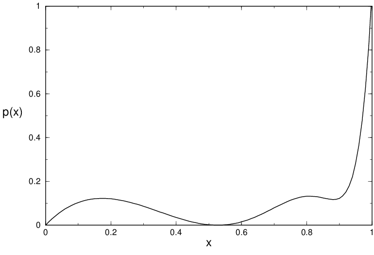
For instance, suppose , , and . The trajectory of is depicted in Fig. 2, together with a detail of the permitted region. The trajectory of crosses the permitted region for values of between , and . The minimum- point on the trajectory segment is the intersection point between the trajectory and the upper boundary of . For this point, it results . The corresponding polynomial , whose graph is depicted in Fig. 3, does not assume negative values between 0 and 1. Hence, the minimum- point on the segment corresponds to a -positive distribution: Then, . The threshold of the corresponding degree distribution is , the value of can be obtained from the function and the values of and can be obtained from the functions and .
| , | , | |||
| -pos. | DE | -pos. | DE | |
| 0.418913 | 0.415774 | 0.341501 | 0.339505 | |
| 0.167565 | 0.180916 | 0.142292 | 0.140214 | |
| 0.266696 | 0.248100 | 0.248395 | 0.259036 | |
| 0.146826 | 0.155210 | 0.267812 | 0.261244 | |
| Thresholds | ||||
| 0.477426 | 0.480325 | 0.488041 | 0.490947 | |
By adopting a similar approach, we fixed , , and looked for the best -positive distribution for and . The optimal distributions were obtained for and , respectively. They are shown in Table II, as well as the optimal check regular distributions obtained by running the DE tool, under the same set of constraints (, and active variable degrees), but without the -positive constraint. The -positive thresholds are only slightly lower than the not -positive counterparts, and the degree distributions are quite similar. Again, the -positive distributions have the advantage represented by the closed-form threshold expression .
V The Binomial Distributions are -positive
In [7], it was shown that capacity achieving sequences of degree distributions for the BEC can be constructed according to the binomial degree distribution. This is a check regular distribution, whose variable distribution is in the form , where , and . Recognizing the binomial degree distributions as part of the -positive family, the following theorem states that this family can achieve the BEC capacity.
Theorem 3
Any binomial degree distribution is -positive.
Proof:
Recall that, for , the -th coefficient of is . For the binomial distribution, it is ω_i λ_i = [(d_c-1)(i-1)-1] α ( α i-1 ) (-1) i α- L ( α L ) (-1) L+1 . Furthermore, it is
where the second equality is due to the fact that , and the last equality to the fact that . Thus, for , , i.e. . It follows , which is always positive for . ∎
VI Conclusion
In this paper, a special family of LDPC degree distributions has been presented. The main feature of these distributions is the possibility to express in closed form their decoding threshold on the BEC, under iterative decoding. More specifically, the threshold admits the simple closed form . This family is a subset of the class of check-regular distributions, and the distributions within this family have been called -positive distributions. A simple necessary condition for a check regular distribution to belong to this class has been obtained, by invoking some known results about the real roots of polynomials.
Three additional properties of the proposed distributions have been highlighted. The first one is their very good threshold under some set of constraints. This property is not general, depending on the specific imposed set of constraints. The second one is the possibility, for particular structures of the variable distribution, to optimize the distribution without necessarily using the numerical optimization tools which are usually exploited. The third one is the possibility to achieve the BEC capacity with sequences belonging to the proposed family.
Acknowledgment
This work was supported by the European Commission under project FP6 IST-001812 PHOENIX. The authors wish to thank Prof. Michele Mulazzani, at the University of Bologna, for useful discussion about polynomials and for suggesting the reference [6].
References
- [1] L. Bazzi, T. Richardson, and R. Urbanke, “Exact thresholds and optimal codes for the binary-symmetric channel and Gallager’s decoding algorithm A,” IEEE Trans. Inform. Theory, vol. 50, pp. 2010–2021, Sept. 2004.
- [2] E. Paolini and M. Chiani, “On the threshold of right regular low-density parity-check codes for the erasure channel,” in Proc. of IEEE Vehicular Technology Conf. Spring, (Stokholm, Sweden), June 2005.
- [3] T. Hehn, A. Dönmez, and J. B. Huber, “Exact thresholds for LDPC codes transmitted over binary erasure channels,” in Proc. of Allerton Conf. on Communications, Control and Computing, (Monticello, USA), Sept. 2005.
- [4] S. ten Brink, G. Kramer, and A. Ashikhmin, “Design of low-density parity-check codes for modulation and detection,” IEEE Trans. Commun., vol. 52, pp. 670–678, Apr. 2004.
- [5] T. Richardson, M. Shokrollahi, and R. Urbanke, “Design of capacity-approaching irregular low-density parity-check codes,” IEEE Trans. Inform. Theory, vol. 47, pp. 619–637, Feb. 2001.
- [6] E. Barbeau, Polynomials. Springer Verlag, 2003.
- [7] M. A. Shokrollahi, “New sequences of linear time erasure codes approaching the channel capacity,” in Proc. of Int. Symp. Applied Algebra, Algebraic Algoritmhs, and Error Correcting Codes (Lecture Notes in Computer Science), M. Fossorier, H. Imai, S. Lin and A. Poli, Eds. Berlin, Germany: Springer-Verlag, pp. 65–76, 1999.
- [8] M. A. Shokrollahi and R. Storn, “Design of efficient erasure codes with differential evolution,” in Proc. of IEEE Int. Symp. on Inform. Theory, (Sorrento, Italy), June 2000.
- [9] M. G. Luby, M. Mitzenmacher, M. A. Shokrollahi, D. A. Spielman, and V. Stemann, “Practical loss-resilient codes,” in Proc. of the twenty-ninth annual ACM symposium on Theory of computing, pp. 150–159, 1997.