Proof of the Double Bubble Conjecture in
Abstract.
The least-area hypersurface enclosing and separating two given volumes in is the standard double bubble.
1991 Mathematics Subject Classification
53A101. Introduction
1.1. The Double Bubble Conjecture
We extend the proof of the double bubble theorem [HMRR02] from to .
Theorem 1.1 (Double Bubble Conjecture).
The least-area hypersurface enclosing and separating two given volumes in is the standard double soap bubble of Figure 1, consisting of three ()-dimensional spherical caps intersecting at degree angles. (For the case of equal volumes, the middle cap is a flat disk.)

In 1990, Foisy, Alfaro, Brock, Hodges and Zimba [FAB+93] proved the Double Bubble Conjecture in . In 1995, Hass, Hutchings and Schlafly [HHS95, HS00] used a computer to prove the conjecture for the case of equal volumes in .
Arguments since have relied on the Hutchings structure theorem (Theorem 3.1), stating roughly that the only possible nonstandard minimal double bubbles are rotationally symmetric about an axis and consist of “trees” of annular bands wrapped around each other [Hut97]. Figures 2 and 3 show examples of “” bubbles, in which the region for each volume is divided into four connected components.

In 2000, Hutchings, Morgan, Ritoré and Ros [HMRR02] used stability arguments to prove the conjecture for all cases in . For , component bounds after Hutchings [Hut97] guarantee that the region enclosing the larger volume is connected and the region enclosing the smaller volume has at most two components. (For equal volumes, both regions need be connected.) Eliminating “” and “” nonstandard bubbles proved the conjecture in . Section 1.2 below sketches their instability argument. ([Mor00] also gives background and a proof sketch.)
In 2003, Reichardt, Heilmann, Lai and Spielman [RHLS03] extended their arguments to , and to higher dimensions provided one volume is more than twice the other. In these cases, component bounds guarantee that one region is connected and the other has a finite number of components. Eliminating bubbles proved the conjecture in these cases.
The same component bounds show that in it suffices to eliminate bubbles (as well as bubbles) to prove the Double Bubble Conjecture. In it suffices to eliminate also bubbles. However, in generally we know only that the larger region has at most three components and the smaller region has a finite number of components [HLRS99].
Here, we extend the methods of Hutchings et al. and Reichardt et al. to prove the Double Bubble Conjecture in for for arbitrary volumes. We prove that nonstandard bubbles are not minimizing for arbitrary finite component counts . The arguments are similar in spirit to those of [RHLS03], except we take advantage of more properties of constant-mean-curvature surfaces of revolution in order to eliminate previously problematic cases. Our arguments also simplify the previous proofs in and because they eliminate the need for component bounds.
1.2. The Instability Argument
An area-minimizing double bubble exists and has an axis of rotational symmetry . Assume that is a nonstandard double bubble. Consider small rotations about a line orthogonal to , chosen so that the points of tangency between and the rotation vectorfield separate the bubble into at least four pieces, as in Figure 4. Then we can linearly combine the restrictions of to each piece to obtain a vectorfield that vanishes on one piece and preserves volume. By regularity for eigenfunctions, is tangent to certain related parts of , implying that they are spheres centered on . In turn, this implies that there are too many spherical pieces of , leading to a contradiction. This is the instability argument of [HMRR02] behind Theorem 4.2.
Therefore, no such useful perturbation axis can exist. By induction, starting at the connected components corresponding to leaves in the tree of Figure 2 we classify all possible configurations in which no such can be found. The induction ultimately shows that must be a “near-graph component stack.” A global argument then finds a suitable . Therefore, cannot in fact be a minimizer.
Having eliminated all nonstandard double bubbles from consideration, the only possible minimizer left is the standard double bubble.
2. Delaunay hypersurfaces
Constant-mean-curvature hypersurfaces of revolution are known as Delaunay hypersurfaces [HMRR02, Hsi82, HY81, Del41, Eel87]. Let be a constant-mean-curvature hypersurface invariant under the action of the group of isometries fixing the axis . is generated by a curve in a plane containing . Put coordinates on the plane so is the axis. Parameterize by arc-length and let be the angle from the positive -direction up to the tangent to . Then is determined by the differential equations
| (1) |
Here, is the slope of , is the planar curvature of with respect to the normal , and is the (constant) mean curvature of with respect to (an average of the planar curvature and the curvature due to rotating about ).

Theorem 2.1 ([HMRR02, Prop. 4.3]).
Let be a complete upper half-planar generating curve that, when rotated about , generates a hypersurface with constant mean curvature. The pair determines up to horizontal translation.
- (1)
If and , then is a curve of catenary type and is a hypersurface of catenoid type.
- (2)
If , then is a locally convex curve and is a nodoid.
- (3)
If , then is a periodic graph over and is an unduloid or a cylinder.
- (4)
If , then is a ray orthogonal to and is a vertical hyperplane.
- (5)
If and , then is a semi-circle and is a sphere.
See Figure 5. The Delaunay hypersurfaces with nonzero mean curvature are the sphere, unduloid and nodoid. If has positive mean curvature upward then it must be a nodoid. If is not graph, then must be either a nodoid or a hyperplane.
Lemma 2.2 (Force balancing [HMRR02, Lemma 4.5]).
Assume that three generating curves , , of Delaunay hypersurfaces meet at a point . Consider normals turning clockwise about . If the curvatures with respect to these normals satisfy , then the forces with respect to these normals satisfy
| (4) |
The lemma follows from Eq. (2).
3. Structure of minimal double bubbles
A double bubble is a piecewise-smooth oriented hypersurface consisting of three compact pieces , and (smooth on their interiors), with a common boundary such that , enclose two regions , , respectively, of given volumes. The work of Almgren [Alm76] (see [Mor00, Ch. 13]) and Hutchings establishes the existence and structure.
Theorem 3.1 ([Hut97, Theorem 5.1]).
Any nonstandard minimal double bubble is a hypersurface of revolution about some line , composed of pieces of constant-mean-curvature hypersurfaces meeting in threes at degree angles. The bubble is a topological sphere with a finite tree of annular bands attached, as in Figure 2. The two caps of the bottom component are pieces of spheres, and the root of the tree has just one branch.
Hence, any minimal double bubble is determined by an upper half-planar diagram of generating curves that, when rotated about , generate the double bubble. By studying these generating curves, we will eliminate as unstable nonstandard double bubbles.
If a double bubble is stable, then for , the mean curvature of with respect to normals pointing into the region is constant over the various smooth pieces of and is called the pressure of , positive by [Hut97, Corollary 3.3]. The pressure difference is the constant mean curvature of with respect to normals pointing from into [HMRR02, Lemma 3.1].
Therefore Lemma 2.2 applies to each vertex, implying.
Claim 3.2.
The outer boundaries of a connected component – between and the outside, – are parts of the same Delaunay hypersurface up to horizontal translation.
Proof.
The boundary pieces have the same pressure and – by applying Lemma 2.2 repeatedly – the same force , so are parts of the same Delaunay hypersurface up to horizontal translation by Theorem 2.1.
More carefully, the proof is by induction on the height of the subtree of descendants of in the associated tree (from Theorem 3.1). Figure 3 provides examples of the cases that arise.
- •
The base case is when has no children, so has just a single piece of outer boundary (e.g., in Figure 3). Then the claim is trivial.
- •
To step the height inductive assumption, assume, e.g., that and have the same force. Force-balancing Lemma 2.2 on vertices and implies that and have the same force with respect to normals pointing into . The same arguments show that and – so all outer boundaries of – have the same force. ∎
Although we will not need it, it is also interesting to remark:
Lemma 3.3 ([HMRR02, Lemma 6.4]).
In a minimizing double bubble for unequal volumes, the smaller region has larger pressure.
4. Instability by separation
Let be a regular stationary double bubble of revolution about axis , with upper half planar generating curves consisting of arcs , with interiors , ending either at the axis or in threes at vertices .
4.1. The map
Definition 4.1.
Define a map that maps to the intersection with of the line orthogonal to at . Let be the ray . Let be the restriction of to the arc . For an endpoint of , define to be the limiting value of approaching , . (For a vertical hyperplane, .)
For short, we will write for , and use similar abbreviated notation for other relevant variables , , , , .
For an endpoint of , note that if and is not a circle or hyperplane (), then for all sufficiently close to , . (This follows, e.g., because is proportional to the force ; see [HMRR02, Remark 5.1].)
4.2. Separating set instability claims
Theorem 4.2 ([HMRR02, Prop. 5.2]).
Consider a stable double bubble of revolution , , with axis . Assume that there is a minimal set of points in with that separates .
Then every connected component of that contains one of the points is part of a sphere centered at (if ) or part of a hyperplane orthogonal to (in the case ).
We sketched the proof of Theorem 4.2 in our introduction Section 1.2. We will apply several useful corollaries of this theorem, taken directly from [RHLS03].
Corollary 4.3 ([RHLS03, Cor. 4.2]).
No generating curve that turns downward past the vertical can have an internal separating set, i.e., two points in the arc, with .
Proof.
Otherwise, by Theorem 4.2, the arc would have to be part of either a circle with center on the axis or a line perpendicular to . But neither turns past the vertical. ∎
Corollary 4.4 ([RHLS03, Cor. 4.3]).
No generating curve that is not part of a vertical line can go vertical twice, including at least once in its interior.
Proof.
Such an arc (a nodoid by Theorem 2.1) has a separating set for some with large enough, contradicting Corollary 4.3. ∎
Corollary 4.5 ([RHLS03, Cor. 4.4]).
Consider a nonstandard minimizing double bubble. Then there is no such that contains points in the interiors of distinct that separate .
Proof sketch.
For , the statement is [HMRR02, Prop. 5.7]. Arguments using “force balancing” show that more pieces of the minimizer are spherical and hence the bubble is the standard double bubble. For , note that a separating set crosses at least one outer boundary. By Theorem 4.2, this boundary is a vertical line, contradicting positive pressure of the regions. ∎
We will consider various nonstandard double bubbles, and show that they violate one of the above corollaries of Theorem 4.2, hence cannot be minimizing.
5. Delaunay hypersurface lemmas
We will need a few more properties of Delaunay hypersurfaces, which can be proven by comparing to certain spheres.
Lemma 5.1.
Consider an unduloid generated by rising to a point where it makes an angle above the horizontal. Then the ray going back down from at an angle of with the unduloid passes completely beneath it to the left of .
Proof.
For , the ray leaves heading to the right, so cannot cross the unduloid to the left. Assume therefore that . (In applications, we will set .) See Figure 6.

Consider the circle centered on the axis and passing through tangent to the unduloid. Note that the ray in question passes entirely beneath the semicircle above the axis; Figure 7. We will show that the unduloid stays above the semicircle to the left of .

Recall Eq. (2) for the force of a constant-mean-curvature surface of revolution with respect to a downward-pointing normal. For an unduloid , while for a sphere (Theorem 2.1). Since at , and are the same, the sphere has higher mean-curvature .
In particular, the planar curvature of at is less than (because the portion of due to rotating about is the same for each), so leaves above . Assume for contradiction that crosses for the first time at a point to the left of . Then the unduloid is steeper than the circle at : , so achieves the angle at some point below .
However, this is impossible; for any angle , the -coordinate at which first reaches , , is no more than the -coordinate at which reaches , . Indeed, (Eq. (3)), so is decreasing moving left, while is constant. therefore reaches some maximum angle . Beyond , turns upward away from the circle, so the curves can only further diverge. But for , the difference in coordinates from to where the curve reaches is
Since is decreasing, while is constant, indeed . ∎
Lemma 5.2.
Consider a smooth curve of length between points and . Let be the angle the curve makes with the horizontal at arc-length from , with and the initial and final angles. Assume . (If we rotate the coordinate system so , then .) Assume and in . Then the line through at angle clockwise from (i.e., at angle above horizontal) passes above .
Proof.
Rotate the coordinate system so without loss of generality and . Then implies that for all ,
Let
where for the inequality we used that is increasing for . Similarly, let
using that is decreasing for . Hence,
is a convex-up curve between and , so it lies beneath the direct line segment , which has higher slope than, and hence lies beneath, the line through at angle above horizontal. ∎
By Theorem 2.1 and Eq. (3), on a clockwise-turning nodoid, provided ; while for an unduloid with increasing to the right, provided .
Corollary 5.3.
Consider an unduloid or nodoid generating curve strictly increasing left to right from to with the notation of Figure 8. Assume and
Then .
Proof.
By Lemma 5.2, the ray (the extension of the normal ) passes above and by assumption it is clockwise from , so it stays above . ∎
Corollary 5.4.
Consider a piece of boundary, arriving at from the left with the notation of Figure 8. Assume and . Also assume that between and . Then .
Proof.
There are three cases, depending on whether is an unduloid, a convex-up catenoid or nodoid, or a nodoid convex-down at . The assumption that between and prevents a nodoid from turning too far around between and .
- (1)
If is an unduloid, then by Lemma 5.1, the ray passes downward beneath , so in particular stays right of . (This remains true if the unduloid passes through one or more minima between and .)
- (2)
If is a convex-up catenoid or nodoid, then convexity implies again that stays right of .
- (3)
If is a convex-down nodoid, then by Lemma 5.2 with again stays right of . (Applying the lemma requires reflecting horizontally and using that turns no more than radians from to .)
In all cases, since leaves clockwise of how leaves , . ∎
6. Rotation notation
A nonstandard minimal double bubble’s generating curves can be classified by the angles at which arcs leave each vertex. For our analysis, it will suffice to know which arcs are leaving from the right and which from the left; there are therefore six cases, each covering radians, which we term “notches.” Incrementing the rotation notch of a vertex corresponds to turning it counterclockwise until an arc passes the vertical, as occurs for from Figure 3 to Figure 9, and from Figure 10(a) to 10(b). The extreme position with an arc leaving a vertex exactly at the vertical divides two consecutive notch cases. If the limiting value of along the vertical arc is (or if the arc is a vertical line), the position is assigned the smaller rotation notch value, and if the limiting value is , the position is given the larger notch value.

The rotation numbers for our earlier bubble example are indicated in Figure 11.

7. Near-graph leaves and bubble stacks
7.1. Near-graph leaves
A “leaf” of a nonstandard minimizing double bubble corresponds to a leaf of its associated tree of Theorem 3.1 and Figure 2. We will use the notation of Figure 12.
Definition 7.1.
A leaf is near graph if vertices and are rotated respectively notches, notches or notches from their positions in Figure 12. (Figure 13 gives examples for the latter two cases.)
We say that a near-graph leaf is right-side up if, with the notation of Figure 12, the region below is inside the bubble; and upside down if the region above is inside the bubble.


Claim 7.2.
For an upside-down, near-graph leaf component, the region containing the leaf must have strictly higher pressure.
Proof.
If has positive pressure up in Figures 12 or 13, then must be a convex-up nodoid. But then the angle constraints at vertices and cannot be satisfied, a contradiction. If there is zero pressure across , then can be a catenoid or a vertical hyperplane, but again neither matches the angle constraints.∎
7.2. Right-side-up, near-graph component stacks
Definition 7.3.
A component stack consists of a base component and all its descendants in the associated tree . The base component cannot be the root component of . A right-side-up, graph component stack is a component stack in which all the associated generating curves are graph, and the root is downward from the base component. A right-side-up, near-graph component stack – or “near-graph stack,” for short – is the same, except for each internal boundary the left vertex can be rotated one notch clockwise or the right vertex rotated one notch counterclockwise.


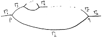
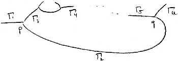
Lemma 7.4.
For a right-side-up, near-graph component stack in a minimizer, with the notation as in Figure 15, .
Proof.
Assume without loss of generality that vertex is rotated as in Figure 15 – if in fact is rotated notches, then flipping the picture horizontally gives the desired positioning.
If (second case of Figure 15), then is a convex-up nodoid since it turns past the vertical, and the ray therefore stays above , implying .
Therefore assume and are rotated as in the first case of Figure 15; . The proof now is by induction on the height of the stack.
If the component stack is just a leaf (height one), then goes from to as in Figure 12. Both . If , then and imply that , too, giving a separating set.
If the component stack has height greater than one, then by induction and to prevent internal separating sets . Since and , again it must that . ∎
Corollary 7.5.
An arc of outer boundary cannot turn downward past the vertical after leaving a right-side-up, near-graph component stack.
Proof.
By Lemma 7.4, . If turns downward past the vertical, then , a contradiction of Corollary 4.5. Similarly cannot turn downward past the vertical. ∎
(Lemma 7.4 is a generalization of [RHLS03, Lemma 7.5], and Corollary 7.5 compares to [RHLS03, Prop. 7.6].)
8. Leaf and component classification
We now classify the types of leaves and general components that may occur in a minimizer. In flavor, this section is similar to the leaf classification [RHLS03, Prop. 7.1] – however, we will complicate things by considering component stacks and not just leaves; and simplify things by applying Corollaries 5.3 and 5.4.
Theorem 8.1.
In a minimizer, every leaf must be near graph, and every component stack of height must be near graph and right-side up.
Proof.
The proof will be by induction on the height of the stack. To reduce repetitive arguments, we will simultaneously consider leaves and component stacks; on a first reading, however, it may be easier to specialize just to leaves. Diagrams will be condensed by using to indicate the possible presence of one or more near-graph leaves or right-side-up, near-graph stacks.
Notation: For leaves we will use use the notation of Figure 12. Cases will be separated according to vertex rotations in notches away from their positions in that diagram. For the base component of a component stack of height , cases will be separated according to vertices’ notches away from their positions in one of the cases of Figure 16. Here, either or is no longer a single arc, but the union of multiple outer boundary arcs (all pieces of the same Delaunay hypersurface by Claim 3.2).
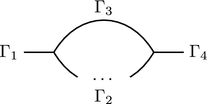
Note also the symmetries; case is symmetrical under relabeling to , and under horizontal reflection to .
The most difficult cases will be (symmetrical to ) and .
Cases and : See Figures 17 and 18(a). This case includes all leaves or base components with and (and if ). A or leaf is near graph, so is allowed in the statement of the theorem. If instead the component is the base of a component stack with one or more near-graph stacks sitting above it, overall we still have an allowed near-graph stack. If it has a near-graph leaf sitting below it, then by Claim 7.2 the leaf’s region has higher pressure. However, must have positive pressure down to match the angle constraints at and , a contradiction.


Case : See Figure 18(b). (With the notation of Section 6, this includes the case in which is a vertical hyperplane.) A right-side-up, near-graph stack cannot be placed along without contradicting Corollary 7.5, since turns downward past the vertical. The presence of upside-down, near-graph leaves sitting beneath beyond where turns past the vertical will not affect our argument.
If is a single piece of arc, then by Corollary 5.4 on , . (If is a vertical hyperplane, then Corollary 5.4 doesn’t apply, but still .) However, , so has an internal separating set, contradicting Corollary 4.3 or Corollary 4.5 (if there is a leaf below ).
In Figure 18(b), is drawn with between and , so it may appear that a near-graph stack cannot be placed on . However, this is not the case; see, e.g., Figure 19. We claim that even if there are one or more near-graph stacks along , still so has an internal separating set.
Letting be the point where turns vertical (), we see that ; is above . By Claim 3.2, the pieces of leaving and leaving are parts of the same Delaunay hypersurface, up to horizontal translation. Let be the first vertex reaches after leaving ; we claim that from to goes above . Indeed, since is the left vertex of a near-graph stack, it must be that ; in particular, . If is an unduloid, then as rises (see Eq. (3)), so is more than from until it reaches the height of . If is a nodoid or a circle, then , yielding the same conclusion.
Therefore, from to goes above ; so there exists along from to , with and . Slide the ray left horizontally to point ; then Corollary 5.4 shows that , so in particular as claimed.
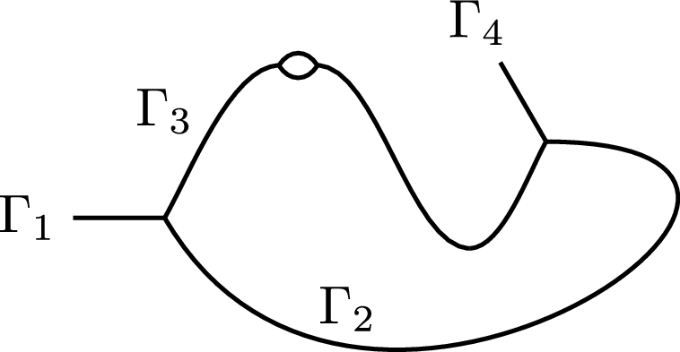
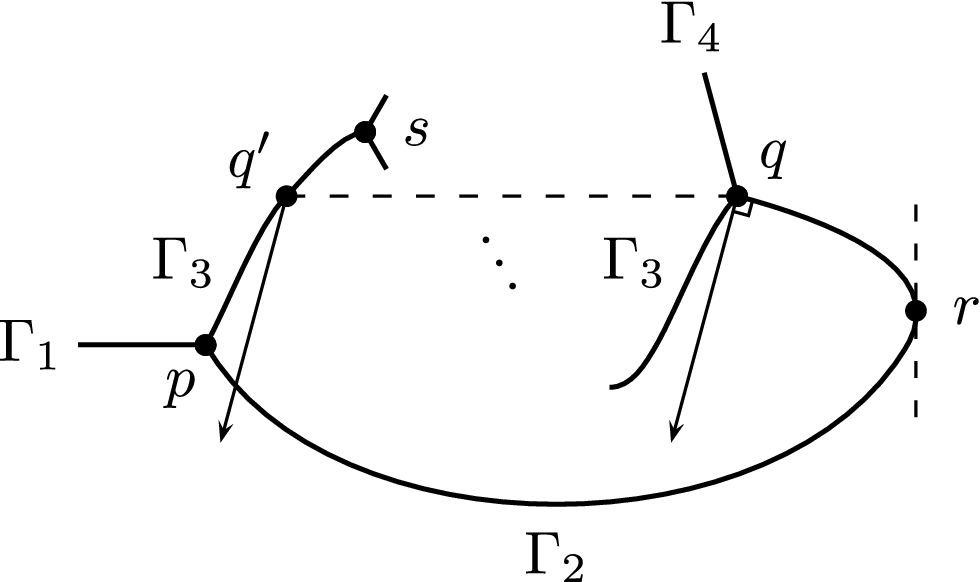
Case or : See Figure 18(c). There cannot be a stack sitting above without contradicting Corollary 7.5, since turns downward past the vertical.
must be a convex-left nodoid (it cannot have any components along it by induction), so the ray stays right of , implying , contradicting either Corollary 4.3 or Corollary 4.5 (if there is a leaf below ).
Cases , and : See Figures 18(d), 18(e) and 18(f). There cannot be a right-side-up near-graph stack above by Corollary 7.5 since turns downward past the vertical. Upside-down, near-graph leaves cannot be placed along without contradicting Claim 7.2. The presence of upside-down, near-graph leaves sitting beneath beyond where turns past the vertical will not affect our argument.
Now . In case or , , while in case , . Regardless, Corollary 4.5 on , , implies .
In turn, this implies that must turn at least radians (i.e., ), and turns at most radians. Indeed, this is necessary by definition in case . In case , it follows since is to the right of , although . In case , it follows since the ray stays above the convex-right nodoid , and .
Next, we argue that . Then since , there is an internal separating set in , contradicting either Corollary 4.3 or Corollary 4.5 (if there is a leaf below ).
Indeed, in case , Corollary 5.4 applies to give . In case or , we may assume that does not go through a minimum and maximum between and – see Figure 20. Therefore, in case or with , is strictly decreasing between and . Corollary 5.3 applies to give .
Finally, it remains to show that in case with . Corollary 5.3 does not apply to in this case, so we need some additional geometry.11 1 [HMRR02, Lemma 5.9] would suffice for this case, and in fact with Corollary 5.3 is enough for all of cases and . However, we will give a slightly simpler argument just for case with . By Lemma 8.2 (below) applied to point with and applied to point with (also ), we get . Since , as desired.
Case : See Figure 18(g). There cannot be a right-side-up near-graph stack above by Corollary 7.5, nor an upside-down near-graph leaf under by Claim 7.2. It remains to eliminate the case of a leaf – we repeat the argument of [RHLS03, Prop. 7.1]. Now . The ray stays left of the convex-right nodoid , so and . This contradicts Corollary 4.5 for , , .
Case or : See Figure 18(h). goes twice vertical, contradicting Corollary 4.4 or Corollary 4.5.
This and symmetrical considerations concludes the argument if either or descends approaching or , respectively. The last remaining case is , in which both and ascend approaching or .
Case or : See Figure 18(i). goes twice vertical, contradicting Corollary 4.4 or Corollary 4.5. ∎
Lemma 8.2.
Let be a point at height above the axis . Let . Drop lines from at angles and from the vertical (Figure 21). Then the difference in the -coordinates of these lines’ intersections with ,
is a strictly increasing function in both and .
Proof.
Simplifying,
and and is decreasing for . ∎

9. Root stability
The “root” of a nonstandard minimizing double bubble corresponds to the root of its associated tree of Theorem 3.1 and Figure 2. The root involves five arcs including two circular caps to either side, as in Figure 22.
Proposition 9.1.
In a minimizer, the child component of the root component cannot be either an upside-down, near-graph leaf, or the base component of a right-side-up, near-graph stack.
Proof.
and are pieces of circles centered on the axis , so , the number of notches , are rotated from their positions in Figure 22 must each lie in .
In particular, neither nor can turn past the vertical to connect to an upside-down, near-graph leaf.
For to be the base component of a right-side-up, near-graph stack, . In case , and , so there is a separating set across , , contradicting Corollary 4.5. Similarly, .
In case , to avoid a separating set between and either or , it must be that , contradicting Lemma 7.4 for the far endpoints of and . ∎
10. Proof of the Double Bubble Conjecture
Proof of Theorem 1.1.
Suppose that the minimizer is nonstandard. Each region has a finite number of components by Corollary 3.1. Consider the minimizer’s generating curves. Theorem 8.1 implies that the root’s child component is either an upside-down, near-graph leaf, or the base component of a right-side-up, near-graph component stack – contradicting Proposition 9.1. Therefore, an area-minimizing double bubble must be the standard double bubble. ∎
Acknowledgements. The author thanks Marilyn Daily for helpful discussions, and thanks Frank Morgan for comments on an early draft of the paper. Research supported by NSF Grant PHY-0456720 and ARO Grant W911NF-05-1-0294.
References
- [Alm76] F. J. Almgren, Jr. Existence and regularity almost everywhere of solutions to elliptic variational problems with constraints. Memoirs A.M.S., 4(165):i–199, 1976.
- [Del41] Charles Delaunay. Sur la surface de révolution dont la courbure moyenne est constante. J. Math. Pures. Appl. Sér 1, 6:309–320, 1841.
- [Eel87] James Eels. The surfaces of Delaunay. Math. Intelligencer, 9:53–57, 1987.
- [FAB+93] Joel Foisy, Manual Alfaro, Jeffrey Brock, Nickelous Hodges, and Jason Zimba. The standard double bubble in uniquely minimizes perimeter. Pac. J. Math., 159:47–59, 1993.
- [HHS95] Joel Hass, Michael Hutchings, and Roger Schlafly. The double bubble conjecture. Elec. Res. Ann. AMS, 1(98-102), 1995.
- [HLRS99] Cory Heilmann, Yuan Y. Lai, Ben W. Reichardt, and Anita Spielman. Component bounds for area-minimizing double bubbles. Technical report, NSF “SMALL” undergraduate research Geometry Group report, Williams College, 1999.
- [HMRR02] Michael Hutchings, Frank Morgan, Manuel Ritoré, and Antonio Ros. Proof of the double bubble conjecture. Ann. Math., 155:459–489, 2002, math.DG/0406017.
- [HS00] Joel Hass and Roger Schlafly. Double bubbles minimize. Ann. Math., 151:459–515, 2000.
- [Hsi82] Wu-Yi Hsiang. A generalization of theorems of A. D. Alexandrov and C. Delaunay on hypersurfaces of constant mean curvature. Duke Math. J., 49:485–496, 1982.
- [Hut97] Michael Hutchings. The structure of area-minimizing double bubbles. J. Geom. Anal., 7:285–304, 1997.
- [HY81] Wu-Yi Hsiang and Wen-Ci Yu. A generalization of a theorem of Delaunay. J. Differential Geom., 16:161–177, 1981.
- [Mor00] Frank Morgan. Geometric Measure Theory: A Beginner’s Guide. Academic Press, third edition, 2000.
- [RHLS03] Ben W. Reichardt, Cory Heilmann, Yuan Y. Lai, and Anita Spielman. Proof of the double bubble conjecture in and certain higher dimensional cases. Pac. J. Math., pages 347–366, 2003.