Dynamic Screening in a Two-Species Asymmetric Exclusion Process
Abstract
The dynamic scaling properties of the one dimensional Burgers equation are expected to change with the inclusion of additional conserved degrees of freedom. We study this by means of 1-D driven lattice gas models that conserve both mass and momentum. The most elementary version of this is the Arndt-Heinzel-Rittenberg (AHR) process, which is usually presented as a two species diffusion process, with particles of opposite charge hopping in opposite directions and with a variable passing probability. From the hydrodynamics perspective this can be viewed as two coupled Burgers equations, with the number of positive and negative momentum quanta individually conserved. We determine the dynamic scaling dimension of the AHR process from the time evolution of the two-point correlation functions, and find numerically that the dynamic critical exponent is consistent with simple Kardar-Parisi-Zhang (KPZ) type scaling. We establish that this is the result of perfect screening of fluctuations in the stationary state. The two-point correlations decay exponentially in our simulations and in such a manner that in terms of quasi-particles, fluctuations fully screen each other at coarse grained length scales. We prove this screening rigorously using the analytic matrix product structure of the stationary state. The proof suggests the existence of a topological invariant. The process remains in the KPZ universality class but only in the sense of a factorization, as . The two Burgers equations decouple at large length scales due to the perfect screening.
pacs
64.60.Ht, 05.40-a, 05.70.Ln, 44.10.+iI Introduction
Many non-equilibrium driven systems display scale invariance in their stationary states, i.e., strongly correlated collective structures without a characteristic length scale limiting the fluctuations. Such correlations typically decay as power laws with critical exponents that are universal. Their values depend only on global issues like dimensionality, symmetry, and specific microscopic conservation laws. The classification of dynamic universality classes and the determination of their scaling dimensions is one of the central issues in current research of non-equilibrium statistical physics Hinrichsen00; Odor04. The one-species asymmetric exclusion processes (ASEP) serves in this context as both the simplest prototype model for driven one-dimensional (1D) stochastic particle flow Ligget85; Spohn91; Schmittmann95 and as a fully discretized version of the 1D Burgers equation (with time and space discretized, and momentum quantized) Halpin95.
In this paper we investigate how the properties of such stochastic flows change with the introduction of additional bulk conservation laws. The generic expectation is that enforcing more conservation laws changes the scaling dimensions. We follow a bottom-up approach. An example of a top-down approach is the current interest in anomalous 1D heat conduction in Fermi-Pasta-Ulam type models (e.g., a chain of anharmonic oscillators Lepri03, or a one dimensional gas of particles in a narrow channel with different types of interactions Grassberger02). The systems are coupled to heat reservoirs on either end. Those are held at different temperatures and thus induce heat flow along the channel. Computer simulations, e.g., using molecular dynamics, show an anomalous thermal conductivity, , , diverging with system size as . The numerical estimates for the value of in the various versions of the process vary between Lepri03; Grassberger02; Wang04. is expected to be universal. From the analytic side, a mode-coupling treatment predicted Wang04-2, while a renormalization analysis of the full hydrodynamic equations predicts , based on Galilean invariance and an assumption of local equilibrium in the heat sector Narayan02. In our study we add conservation laws to the Burgers equation instead of coarse graining down from full hydrodynamics.
The equivalences between ASEP, KPZ growth, and the Burgers equation are well known Halpin95. ASEP is usually interpreted as a process for stochastic particle transport, while the Burgers equation
| (1) |
represents the evolution of a (vortex free) velocity field , and conserves momentum only Burgers74. The interpretation of ASEP as a fully discretized Burgers equation poses some conceptional issues. Due to the full quantization of the momenta in ASEP, in units of , it can appear that the process also conserves energy. A careful discussion Marcel shows that energy is conserved between updates but fluctuates during each update. Therefore ASEP is a genuine fully discretized implementation of the Burgers equation from this direct point of view as well. In section II we discuss how to impose conservation of particles in addition to conservation of momentum. This leads naturally to the two-species ASEP known as the Arndt-Heinzel-Rittenberg (AHR) model Arndt98; Arndt99. This process has been the focus of intensive studies, but its dynamic scaling properties seem to have been ignored. Instead, the stationary state properties have been center stage, in particular its clustering, and that it can be constructed exactly using the so-called matrix product ansatz method Rajew00; Kafri02; Schutz03; Kafri03; Evans05.
We establish that the introduction of this additional conservation law to ASEP does not change the universality class, but it does so in a rather intricate manner. KPZ scaling changes to (KPZ)2 type scaling. The AHR process can be interpreted as a coupled Burgers and diffusion equation, conserving both mass and momentum; or as two coupled Burgers equations, one for positive and negative momentum quanta separately. The latter point of view turns out to be the most productive. At large length scales the coupling vanishes and the process factorizes, in terms of quasi-particles, into two decoupled Burger processes. This is achieved by means of perfect screening of fluctuations in the stationary state. We observe this numerically from the behavior of the two-point correlators (sections IV and V). The stationary state of the model is known to satisfy the so-called Matrix Product ansatz Arndt98. We use that property to prove analytically that the perfect screening is rigorous (section VI). In sections IV and V we present also direct numerical evidence that the dynamic critical exponent is indeed the same as in KPZ, , using the time evolution of the two point correlators. The conventional methods fail due to time oscillations. This might be the first example of such a numerical dynamic analysis in terms of correlation functions.

II The AHR model
Our aim is to construct a generalization of ASEP describing a process where particle diffusion and the Burgers equation are coupled to each other. Energy will not be conserved. The particles in such a model need to carry an internal degree of freedom, representing momentum. A site could be in four states. It would be empty () or be occupied by a particle () with momentum . Particles with (-1) momentum would hop with a right (left) bias. Some reflection on the nature of the passing processes (the collisions) shows that we can remove the zero momentum state of particles, without loss of generality Marcel.
This then leads naturally to the two-species ASEP known as the Arndt-Heinzel-Rittenberg (AHR) model. The conventional interpretation of this process is in terms of diffusion of charged particles in an electric field. Two species of particles with opposite unit charge hop in opposite directions along a 1D lattice ring, driven by the electric field.
| (2) |
Each site can be in 3 states, , with () representing the right (left) moving species and an empty site. is the free directed hopping rate (the electric field) and the passing rate of opposite charged particles. In our study, the numbers of and particles on the ring are chosen to be equal. Compared to the conventional single species ASEP, this process has two local conservation laws instead of one; both species are conserved independently.
In the coupled diffusion-Burgers equation interpretation of the same process, the charge represents a quantum of momentum moving in opposite direction as illustrated in Fig.1. No driving force is present, because the preferred hopping direction represents the total derivative in the Navier-Stokes equation, just as in the single species ASEP. Similar to ASEP, energy is not a conserved quantity: The energy of particles is conserved between updates but fluctuates during the updates. That leaves particles in different places than where they would have been if energy were conserved Marcel.
The AHR model reduces to the spin (momentum quanta) representation of ASEP in the high density limit where vacant sites are absent. There, the particle density can not fluctuate anymore, and the process falls thus back to the Burgers equation with only one conservation law. This limit is singular. The AHR process is not the generic generalization of ASEP in the sense of the KPZ and Burgers equation. The proper generalization would be the so-called restricted solid-on-solid (RSOS) model (Kim-Kosterlitz model) where and pairs can be annihilated and created. Those processes conserve momentum. The () particles represent up (down) steps in the KPZ type interface, the free hopping rate represents step-flow. Growth at flat terraces is blocked in the AHR process, except for the deposition of vertical dimers (with rate ) in single particle puddles. Fig.1 illustrates this.
This means that from the KPZ point of view the AHR process represents a growing interface where the number of up and down steps are individually preserved. Whether this local conservation law changes the scaling dimensions on large scales is the central issue we address here. From the KPZ perspective, your initial guess would probably be “no”, and from the lattice gas perspective “yes”. Our results presented below confirm the “no”, but in rather subtle manner, the universality class is “(KPZ)2” instead of simple KPZ.
The AHR model has been widely studied recently, with as focus the structure of its stationary state Arndt98; Arndt99; Rajew00; Kafri02; Schutz03; Kafri03. We are not aware of any previous dynamic scaling analysis. The stationary state shows strong clustering, as function of decreasing passing versus free hopping probability, . Stretches of “empty” road are followed by high density clusters. These are mixtures of and particles. We will identify the amount of mixing with the quasi-particles and the cluster size with the screening length.
The passing of and particles resembles collisions. The ratio controls the duration of the collision (the softness of the balls). This passing delay creates queuing and is the origin of the clustering. The full AHR model includes a reverse-passing probability , ((; particles switching position in the direction opposite to the electric field). That enhances the clustering even more. We limit ourselves here to the version of the model.
The clustering extends over such large length scales, in specific ranges of and , that the possibility of a phase transition into a macroscopic clustered stationary state has been the major issue Arndt98; Arndt99. Macroscopic cluster condensation (infinite sized clusters) have been shown to be impossible using the analytic matrix product ansatz Rajew00 and also using an approximate mapping onto the so-called zero range process Kafri02. The cluster size remains always finite, but the maximum value can be far beyond all computation capabilities Rajew00.

III The Phase Diagram
Fig.2 shows the phase diagram of the AHR model as function of and (conserved) global average density . It contains three special lines: , , and , respectively.
Along the line all sites are fully occupied and the process reduces to the singe-species ASEP. From the perspective of the AHR process as modeling two coupled conserved degrees of freedom, momentum and density, the density sector freezes out, leaving only the Burgers equation. The limit is therefore anomalous, and this line is not the proper backbone of the phase diagram. The dynamic scaling exponent is equal to along this line, but that does not need to extend to .
The line and the interpretation of the AHR process in terms of two coupled Burgers equations form the true backbone of the phase diagram. At , the process reduces to a single-species ASEP in two different ways. If the particles choose to be blind to the difference between an empty site and a particle, they see at no difference between a free hop and a passing event, and thus experience pure single species ASEP scaling. The same is true in the projected subspace where particles are blind to the difference between empty sites and particles. These subspaces are not perpendicular and the process does not factorize into two independent ASEP processes. Correlations exist between the and particles, resulting in clustering. We will study this numerically in the next section and find that at large length scales the process factorizes after all, into .
At the particles can still pretend to be blind to the other species, but then experience updates where the hopping probability inexplicably changes from to . These events are random, but not uncorrelated. For the clustering increases and for decreases. The line is special; there the clustering vanishes accidentally altogether.
IV Dynamic Perfect Screening at
Our investigation of dynamic scaling in the AHR model started with an attempt to measure the dynamic critical exponent in the conventional manner, i.e., from the time evolution of the interface width starting from a flat or a random initial state. Recall that the AHR model is a RSOS type KPZ growth model with conserved number of up and down steps. It turns out that this interface width oscillates in time while evolving toward the stationary state, as illustrated in Fig.3.
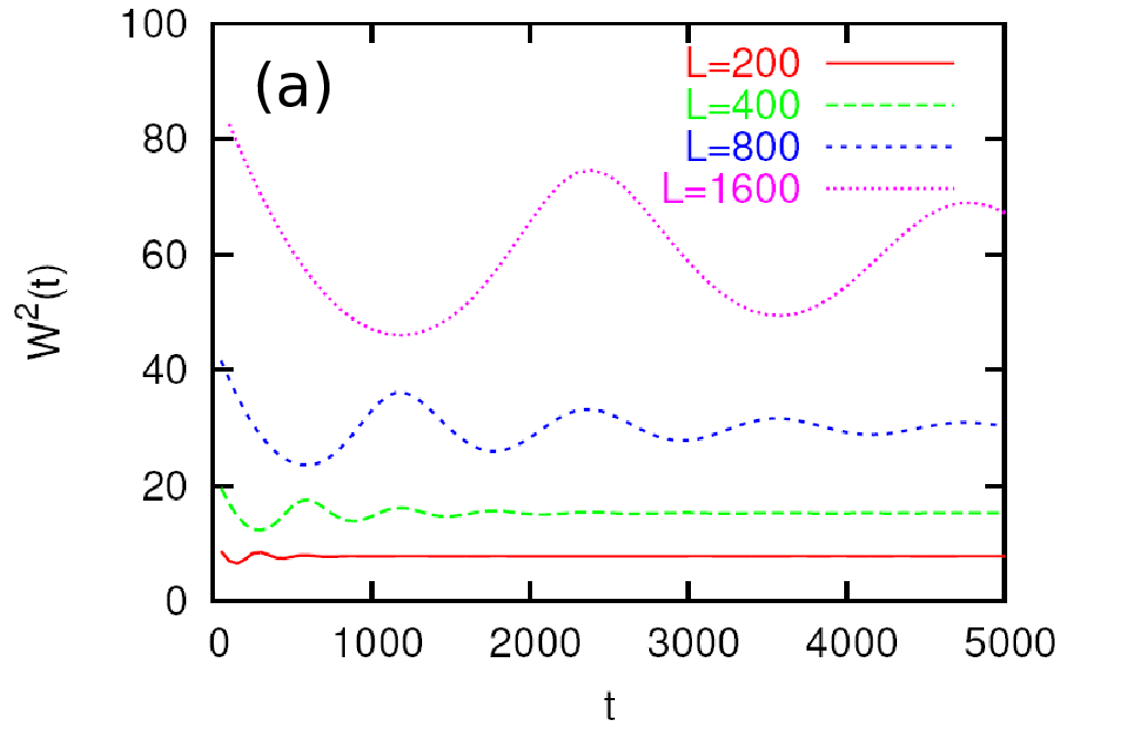

The flat initial state evolves roughly in accordance with conventional scaling, i.e., as , with , at intermediate times and saturating at (with the stationary state roughness exponent), but the oscillations on top of this behavior are too strong to accurately determine . These oscillations reflect the additional conservation law, and are tied to traveling wave packets propagating in opposite directions and meeting again after traveling around the lattice ring.
For the resolution of this problem we turn our attention towards these wave-packets themselves, by monitoring the manner they spread in time. This is achieved in terms of the two-point correlators
| (3) |
and and , where is the number operator for particles at site and at time . The perfect screening phenomenon in the stationary state emerged while we tested this novel method. In this section we first present and discuss perfect screening and then present the numerical analysis of the dynamic exponent, both at .
IV.1 Stationary State Correlation Functions
In the stationary state, the correlation function
| (4) |
decays exponentially toward zero. Figs.4-5 illustrate this, using MC simulations for periodic boundary conditions for small rings, . The correlation function decays exponentially for and is zero for . Correlations are absent at , because after passing, and particles hop away from each other, and (at ) do not communicate with each other anymore.

The correlation length is rather short in Fig.4, , but increases with density along the line. The most significant aspect is not the correlation length, but the absence of any finite size scaling offset for and .
The absence of this offset is quite surprising. It indicates a “perfect screening” localization type phenomenon in the fluctuations. To appreciate this, consider the two-point correlation in a random disordered state, like the single species ASEP stationary state. The and correlators in our model have exactly that form at because each couples only to one of the two projected single species ASEP subspaces. Such correlators are -functions (with negative offsets) because periodic boundary conditions imply rigorous global conservation of the total number of particles, and impose the condition that the total area underneath is exactly equal to zero.
Another way of viewing this starts by realizing that can be interpreted as the probability to find a particle at distance from a tagged particle at site . The tagging removes an amount of probability from corresponding to the (untagged) probability of finding a particle at . This amount is redistributed over the chain. In general, we would expect that part of this expelled probability remains localized near , represented in by the area underneath the exponential; and that the remainder is distributed uniformly over the chain in delocalized form, represented by a uniform type finite size offset in . For uncorrelated -function type correlations all of it is delocalized, such that . Our numerical simulations, see Fig.5, put a bound on the delocalized amplitude; e.g., at for . The delocalized fraction is zero within the MC noise.

So surprisingly, in our process all the excluded probability is localized, such that
| (5) |
for all . A person riding on top of a specific particle and wearing glasses that filter out the particles, observes a perfect single species ASEP in terms of the particles. Without glasses she notices however an excess of particles in front of her. This cloud of size has on average an excess mass equal to .
IV.2 Factorization from Perfect Screening
The above perfect screening implies that the AHR process at behaves at coarse grained scales as two decoupled single species Burgers equations. This factorization is easily recognized in the interface growth representation. Recall that the particles represent up-steps and the particles down steps, and that the number of both are conserved. Perfect screening means factorization into two decoupled KPZ interface growth processes at length scales (one where down-steps are being ignored and the other where the up-steps are ignored).
The interface width of the full model over a section of the interface of length can be expressed in terms of the two-point correlators as
| (6) | |||||
and are -functions at and their finite size offsets are absent in the thermodynamic limit ,
Moreover, at length scales much larger than the screening length, , the cross-correlator area reduces to by perfect screening, such that the contributions vanish completely,
| (7) | |||||
The square of the full interface width is thus equal to the sum of the squared interface widths in the two projected subspaces at . The two coupled Burgers equations behave independently at length scales .
IV.3 Dynamic Exponent from
Fig.6 shows the time evolution of the correlation function starting from an initial uncorrelated disordered state (a -function with a finite size off-set). The build-up of the cluster of particles in front of the tagged particle requires only a short time span . The build-up of this surplus is mirrored by the build-up of a depletion layer behind the particle (particle numbers are locally conserved). After the screening cloud at is fully established, , the depletion packet detaches from and travels to the left. This traveling wave packet belongs to one of the two projected single species ASEP subspaces and therefore should spread in time with KPZ dynamic exponent as . The Gaussian form
fits the wave packet very well Leven except at times close to where it is slightly skewed. The packet’s group velocity, , follows the expected value , i.e., twice the group velocity of fluctuations in the or sector single species ASEP. ( is the relative velocity of fluctuations in the and sectors respectively, propagating in opposite directions.) The traveling depletion wave packet moves around the ring while broadening. It collides after one period with the screening cloud. They split-off again. This keeps repeating itself, until the broadening has spread all over the ring and cancels out against the global finite scaling offset of the initial state.

Fig.7 shows the time evolution of the width of the wave packet and its height . They obey power laws: and . From these, we obtain estimates for the dynamic exponent , and Fig.8 shows the finite size scaling behavior of these estimates. They converge to , consistent with the expected KPZ value . This confirms that this novel way for determining works well.


V Dynamic Screening at
The correlation functions and take more intricate shapes away from the line. Remarkably, as we will discuss next, this variety of shapes convert back into the simple shapes of using a quasi-particle representation. We discovered this numerically, as presented in this section, and then proved it analytically, as presented in the next section. The properties at the line, perfect screening between particles of opposite charge and uncorrelated disordered stationary state statistics in the two projected subspaces, extend thus to all in terms of quasi-particles, and the final conclusion from this is that the process factorizes into (KPZ)2 everywhere for all .
V.1 Stationary State Correlation Functions
Fig.9 shows the and correlators for various values of . Compared to the shapes, develops correlations at , and changes from a -function into a symmetric correlated shape. This can be explained qualitatively as follows. At , the and particles can not choose to be blind with respect to each other anymore. Additional correlations build-up compared to the baseline behavior:
At the passing versus hopping rate is reduced. The screening cloud at in therefore grows (the clustering is stronger). This enhanced screening cloud at , results in short range correlations between alike particles as well; develops positive tails. This is a second order effect. Those particle correlations in turn induce positive correlations in for . This is a third order effect, and thus an order of magnitude further down.
At the passing rate is enhanced with respect to the baseline behavior. The screening cloud in is thus smaller than at . The correlations in are indeed negative, and represent a reduced probability to find alike particles near each other. This reduced probability makes it less likely to find particles behind the tagged particle, at . If those particles had been there, they would carry smaller screening clouds in front of them. Their absence therefore creates still positive correlations between particles at and the tagged one.
At the stationary state is fully disordered Arndt98, the clustering vanishes and all correlation functions reduce there to -functions. At the correlation tails re-emerge, but with opposite signs.


V.2 Dynamic Exponents from and
We examine the temporal evolution of and using MC simulations, just as we did in the case. The initial states are prepared to be uncorrelated and disordered. As shown in Fig.10, two wave-packets appear, with different amplitudes, but moving in opposite directions with the same speed. The wave-packets in are strongly coupled to those in . These traveling clouds are generated by the same type of mechanism as the one at , i.e., the result of the rather fast build-up of the screening clouds near the tagged particle, reflected by the short distance correlations in the stationary state. Both traveling clouds are mixtures of and particles, with non-zero projections in both and .


Once the clouds are detached from , they move independently of each other in opposite directions; just as at . The process factorizes again. But there is no a priori reason why these mixed traveling clouds at should spread as in pure KPZ. However, they do. In our MC simulations they spread, e.g., at , , and , with and at , , and with . Fig.11 and 12 shows strong finite size corrections to the scaling in the dynamic exponents, but the limiting behavior is clear.


Moreover, at , the stationary state is totally uncorrelated and disordered (and the temporal evolutions of the correlation functions therefore do not involve traveling wave packets). We can apply the conventional method to estimate the dynamic exponent. The temporal evolution of the interface widths (see Fig.(13) and (14)), yields .


V.3 Perfect Screening in the Quasi-Particle Representation
If indeed the dynamic exponent retains (KPZ)2 type value at as suggested by the above numerical results, then there might be a quasi-particle description in which the process factorizes at large length scales and in which the fluctuations are perfectly screened, just as at . We found such a description, first numerically as described here, and then rigorously analytically in the following section. This implies the process obeys scaling everywhere. In terms of quasi-particles the dynamic process fully factorizes into two KPZ processes at large coarse-grained scales.
Consider the stationary state correlation functions in Fig.9 and 10: the correlation functions decay to type finite size scaling off-sets. The area underneath for , the area underneath at (equal to the same for ) and the area underneath for obey empirically the relation , for all , typically with a numerical accuracy, . (The areas are measured with respect to the offsets.)
This special balance in the areas relates to a specific amount of mixing between and particles in the clouds, and suggests (a much stronger property) the existence of a quasi-particle representation,
| (8) |
with the number operator for and particles and
| (9) |
in which the correlation functions and , defined as
| (10) |
with reduce to the same shapes as the particle correlators at (where is a -function and has only one tail and shows perfect screening between quasi-particles of opposite charges).
The mixing ratio varies from at (with and ); to =1 when , and to when . Fig.15 shows lines of from our analytic expression in section VI.6. Our numerical results are completely consistent with this. The mixing strength increases with density , and becomes indeterminate at the line , where all sites are fully occupied. At the stationary state is totally disordered, but does not vanish since and remain strongly correlated dynamically Schutz04. Both and go to zero and change sign across the line.

VI Perfect Screening and the Matrix Product Stationary State Structure
In this section, we prove analytically the perfect screening of the (quasi-particles) pair correlators, using the matrix product ansatz (MPA) structure of the stationary state. The proof applies to all , but for clarity we split-up the discussion. First we review briefly the general properties of MPA stationary states. Next, we present the proof at , and finally generalize it to all in terms of quasi-particles.
VI.1 MPA Type Stationary States
Stationary states of stochastic dynamic processes are typically very complex with intricate long-range effective interactions between the degrees of freedom (when writing the stationary state in terms of effective Gibbs-Boltzmann factors). The long-range aspect is important; 1D driven stochastic processes can undergo non-trivial phase transitions, while 1D equilibrium degrees of freedom with short-range interactions can not. MPA states are linked to equilibrium distributions and therefore lack long-range correlations.
MPA stationary states are of the form Arndt98; Arndt99; Rajew00:
| (11) |
with in our case . This structure resembles closely the transfer matrix formulation of partition functions in one dimensional (1D) equilibrium statistical mechanics. Consider for example a one dimensional Ising model, with spin degrees of freedom at sites , that interact as
| (12) |
and with a degree of freedom on every bond such that bond energy can have three distinct values. In that case, the are transfer matrices and the stationary state probability for the yet unrelated stochastic dynamic process is the Ising equilibrium partition function for a given configuration,
| (13) |
The normalization factor
| (14) |
is the canonical partition function of the annealed random bond 1D Ising model. The stochastic driven non-equilibrium dynamics typically imposes constraints on the degrees of freedom. In our dynamic process the number of each species of particle, , is conserved independently. This is denoted by in eq.(14).
The variables do not couple to each other directly in eq.(13); all correlations between degrees of freedom are mediated by the Ising field . The search for a possible MPA structure of the stationary state is therefore the search for the existence of a representation in which all correlations between the original degrees of freedom are carried by a new auxiliary field and expressed as short-range interactions between those new degrees of freedom. Those auxiliary degrees of freedom can take any form, not just Ising spins, because the rank of the matrices and their symmetries can be arbitrary. For example in our case, the rank will be infinite, and the auxiliary field can be interpreted as (integer valued) interface type degrees of freedom, denoted as .
The transfer matrix product structure, eq.(11), implies that those auxiliary degrees of freedom interact by nearest neighbor interactions only. This is actually unfortunate, because in short-ranged 1D equilibrium systems, like eq.(13), spontaneous broken symmetries and phase transitions are impossible. Therefore, master equations with MPA stationary states have at best dynamic phase transitions with trivial scaling properties (associated with an abrupt change in the -representation). For example, MPA representations of directed percolation or directed Ising type processes can not exist, because both are believed to have transitions with complex scaling dimensions. Still, the MPA method has been proved to be a powerful tool, its algebraic structure is very elegant, and a surprisingly large class of 1D stochastic dynamic processes have a MPA type stationary state.
Boundary conditions play an important role. Eq.(14) is a canonical partition function, where the number of and particles are each conserved. Consider instead the generating function
| (15) | |||||
with
| (16) |
This would be the grand canonical partition function of, e.g., the above annealed random bond 1D Ising model in case of periodic boundary conditions. are the fugacities of the particles. The equivalence between the ensembles in the thermodynamic limit is ensured in the equilibrium interpretation, where the details of how the particle reservoirs couple to the system does not have to be addressed. This is different in the interpretation of the MPA as the stationary state of a driven stochastic process. Dynamic processes are very sensitive to boundary conditions. For example, a process with open boundary conditions and reservoirs at the edges conserves the number of particles everywhere inside the bulk, and behaves very different from the one where the reservoirs couple directly to every site. Not surprisingly therefore, the MPA method only applies to the stationary state; the introduction of the auxiliary field does not address the stochastic dynamics, nor the temporal fluctuations in the stationary state. For periodic boundary conditions, as in our case, the grand canonical partition function eq.(15) represents an ensemble of dynamic systems, each with periodic boundary condition systems, and fixed values of and , weighted with respect to each other by the fugacity probability factor. In this sense the ensembles are equivalent in the thermodynamic limit. In our discussion below we use the grand canonical ensemble. The correlation functions for are evaluated then as
| (17) |
in the thermodynamic limit, with and the right and left eigenvectors of the largest eigenvalue of the operator defined in eq.(16). The correlator at , , poses somewhat of a problem. It can not be expressed as simple as this due to the intrinsic off-diagonal character of the above operators. At this is not an issue, because . However, that will not be true anymore for the quasi-particles at .
VI.2 Quadratic Algebra
The first step in identifying whether the stationary state of a stochastic process might have a MPA structure, is to insert Eq.(11) into the master equation. If lucky, the condition of stationarity can be expressed as simple algebraic conditions on the transfer matrices. The MPA structure of our process has been studied extensively recently Arndt98; Arndt99; Rajew00; Kafri02; Schutz03; Kafri03. From those studies we know that the three must obey the quadratic algebra:
| (18) |
with and arbitrary yet unspecified parameters. These conditions apply to the entire phase diagram, for all . The next step is to find explicit representations of the that satisfy eq.(18), using the freedom in choice of the parameters . In general the rank of the does not close, but remains infinite. The rank is finite only along special lines in the phase diagram. Fortunately, for our purposes we do not need closure; the quadratic algebra structure itself is sufficient to prove perfect screening.
Our process is invariant under simultaneous inversion in space and of charge in the case that the numbers of and particles are balanced. This suggests we look for a realization of the algebra with operators satisfying and . This invariance is valid in the subspace and Arndt98, where the quadratic algebra reduces to
| (19) |
VI.3 The Quadratic Algebra
At , the quadratic algebra of Eq.(19) is easily checked to be satisfied by the operators Arndt99
| (20) |
The rank of these matrices is infinite. The auxiliary degrees of freedom are (positive only) integer valued “height variables” . is the projection operator onto the state, and are the raising (lowering) operators, .
We need to determine the eigenvalues of the grand canonical transfer matrix, eq.(16),
| (21) |
This matrix has several interpretations. It is the transfer matrix for the equilibrium partition function of a one dimensional interface in the presence of a substrate (all are excluded) with a short range attractive potential at ; like a substrate. Such an interface layer is thin and non-rough. It is also the time evolution of a 1D random walker (with playing the role of time and that of space) in half space, and an on-site attractive interaction at site . Such a random walker is localized. The latter can be presented also as localization of a single quantum mechanical particle hopping on a semi-infinite chain with a -function attractive potential at the first site,
| (22) |
with .
This simple Hamiltonian has one single bound state and a continuum spectrum of extended states. The calculation of the eigen-spectrum is elementary and straight forward. The eigenstates, , satisfy the equations:
| (23) |
Bound states have the generic form
| (24) |
Substitution in Eq.(23) yields only one bound state, with energy , such that
| (25) |
and normalization
| (26) |
is equal to .
The extended eigenstates are scattered waves, with
| (27) |
The eigenvalue equations at yield the energy spectrum, , with , such that
| (28) |
and those at yield the phase shift ,
| (29) |
The normalization factor
| (30) |
is proportional to the rank of the matrices , and thus strictly speaking infinite; will drop out in our calculations below. The component is easily evaluated:
| (31) |
VI.4 Perfect Screening at
Perfect screening implies that
| (32) |
i.e., that the sum over of the correlator Eq.(17),
| (33) |
is equal to the right hand side of Eq.(32),
| (34) |
with , using that the bound state is also an eigenstate of , . In our specific case the density is simply equal to , but we like to keep the derivation as generic as possible.
We need to demonstrate that this sum rule is valid in the thermodynamic limit, and track carefully any terms that scale as system size . For example, as discussed already in detail above, the sum rule is trivially true for periodic boundary conditions, but then does not imply perfect screening, because any unscreened surplus can be spread out over the entire lattice in the form of a background density.
Define , as the projection operator onto the bound state, and rewrite Eq.(17), as
| (35) |
The bound state does not contribute to the correlators inside the sum. Therefore we can project out the bound state from and then perform the summation
| (36) | |||||
(The single outside the summation originates from the contribution.) We can remove and from the above equation, because the bound state is also an eigenstate of the lowering operator, ,
| (37) |
writing , and using that is the projection operator onto the first site, and also that has no projection onto .
The sum rule we seek is now reduced to the identity
| (38) |
with . The left hand side is easily evaluated, using Eq.(31) and that ,
| (39) |
This is an elementary contour integral along the unit circle in the complex plane, with a double pole at within the circle in addition to a single pole at . The integral is indeed equal to , the right hand side of Eq.(37) ( and ).
VI.5 Quadratic Algebra at
The proof of perfect screening for general follows the same pattern as at . The operators obeying the quadratic algebra conditions, Eq.(19), are again expressed in terms of raising and lowering operators , Arndt98; Arndt99; Rajew00; Kafri02; Schutz03; Kafri03
| (40) |
where and . The transfer matrix retains its form
| (41) |
with modified Hamiltonian,
| (42) | |||||
and with . This is again a one-dimensional single particle hopping process in a half-space, . Compared to Eq.(22) for , the attractive potential at site deepens for (reducing the clustering and correlation lengths). The novel element is the modified hopping probability between sites and . There is still only one bound state
| (43) |
with the same functional form for the bound state energy as before, Eq.(25).
VI.6 Quasi-Particle Representation
We can now identify the exact form of the ratio in the quasi-particle representation, eq.(8). The representation mixes the operators in Eq.(40) as
| (46) |
The projection operator, , and the transfer matrix are invariant. The latter implies .
The quasi-particle two-point correlation functions take the same form as the particle correlators at . In particular, the quasi-particle correlation function is zero for all . This is true when the bound state is also an eigenstate of :
| (47) |
Inserting the bound state, Eq.(43), yields
| (48) |
and
| (49) |
The lines of constant are shown in Fig.(15). (Insert the above equations for , , and the relation between and .) The contours coincide with our numerical results.
VI.7 Perfect Screening at
The final step is to prove perfect screening in terms of the quasi-particles:
| (50) |
The left hand side reduces to exactly the same form as Eq.(37), using the exact same steps, because the bound state is an eigenstate of just like the particle operator at ; that is all we used there. The right hand side is different, because is not zero anymore. Since , it is still true that . Therefore the sum rule equation, Eq.(38) now takes the form
| (51) |
with, as before, . The summation on the left leads again to a type contour integral. It still has only two poles inside the unit circle: one double pole at and one single pole at (with the second root of Eq.(43).) The result is indeed equal to the right hand side after inserting the proper expressions for the various eigenvalues and some not very pretty algebra.
VII Results and Conclusions
We have studied the two-species asymmetric exclusion process (ASEP) to determine whether the addition of a local conservation law changes the dynamic scaling properties. In the Burgers (hydrodynamics) context the process conserves both momentum and density. In the KPZ context it represents interface growth where the numbers of up and down steps are conserved. In the ASEP context the particle numbers of both species are conserved.
We find that the dynamic scaling exponent retains the KPZ value. The AHR process factorizes at scales larger than the clustering length scale, , into two-independent KPZ processes. At , where the passing and hopping probabilities are equal, this factorization occurs in terms of and particles, while at it is established in terms of quasi-particles. This factorization expresses itself as perfect screening between the two species of quasi-particles. , the screening length, coincides with the clustering length scale and represents the crossover length scale between single KPZ scaling (within each cluster) and factorized type scaling.
The conventional method for measuring the dynamic exponents in simulations in terms of the time evolution of the interface width fails in this process due to the presence of time-oscillations with a period proportional to the system size; quasi-particles fluctuations have non-zero and opposite drift velocities. Instead, we determined the dynamic scaling from the two-point correlation functions. This might be the first time that it is done in this manner.
The stationary state of this process has been studied extensively in the recent literature, because it obeys the so-called matrix product ansatz (MPA). We used this to prove rigorously the factorization of the fluctuations in terms of quasi-particles. This previously unknown feature of the algebraic structure of the MPA method needs to be understood better, in particular in the context of clustering phenomena in general.
The perfect screening phenomenon is clearly a topological feature. The above presentation only partially exposes those topological properties; by bringing the perfect screening condition into the form of Eqs.(38) and (51). The right hand sides of both equations only involve bound state properties. Their left hand sides however involve a summation over all extended states; i.e., their projections onto (). The poles of the contour integral links this to the bound states and the quasi-particle mixing. The formulation of a general proof is important because, if topological, the prefect screening and (KPZ)2 scaling at large length scales will be generic features, valid to many more processes with clustering. Its limitations can teach us when and how novel type dynamic scaling sets in.
Acknowledgment – This research is supported by the National Science Foundation under grant DMR-0341341.
References
- (1) H. Hinrichsen, Adv. Phys. 49, 815 (2000).
- (2) G. Ódor, Rev. Mod. Phys. 76, 663 (2004).
- (3) T. M. Ligget, Interacting Particle Systems (Springer-Verlag, New York, 1985).
- (4) H. Spohn, Large Scale Dynamics of Interacting Particles (Springer-Verlag, New York, 1991).
- (5) B. Schmittmann and R. K. P. Zia, Statistical Mechanics of Driven Diffusive Systems, vol. 17 of Phase Transitions and Critical Phenomena (Academic, New York, 1995).
- (6) T. Halpin-Healy and Y. -C. Zhang, Phys. Rep. 254, 215 (1995).
- (7) S. Lepri, R. Livi, and A. Politi, Phys. Rev. Lett. 78, 1896 (1997); S. Lepri, R. Livi, and A. Politi, Europhys. Lett. 43, 271 (1998); T. Prosen and D. K. Campbell, Phys. Rev. Lett. 84, 2857 (2000); S. Lepri, R. Livi, and A. Politi, Phys. Rev. E 68, 067102 (2003); S. Lepri, R. Livi, and A. Politi, Phys. Rep. 377, 1 (2003).
- (8) P. Grassberger, W. Nadler, and L. Yang, Phys. Rev. Lett. 89, 180601 (2002); T. P. G. Casati, Phys. Rev. E 67, 015203 (2003); J. M. Deutsch and O. Narayan, Phys. Rev. E 68, 010201 (2003).
- (9) J. S. Wang and B. Li, Phys. Rev. E 70, 021204 (2004); T. Hatano, Phys. Rev. E 59, R1 (1999).
- (10) J. S. Wang and B. Li, Phys. Rev. Lett. 92, 074302 (2004).
- (11) O. Narayan and S. Ramaswamy, Phys. Rev. Lett. 89, 200601 (2002); T. Mai and O. Narayan, Phys. Rev. E 73, 061202 (2006).
- (12) J. M. Burgers, The Nonlinear Diffusion Equation (Riedel, Boston, 1974).
- (13) M. den Nijs, unpublished.
- (14) P. F. Arndt, T. Heinzel, and V. Rittenberg, J. Phys. A 31, 833 (1998).
- (15) P. F. Arndt, T. Heinzel, and V. Rittenberg, J. Stat. Phys. 97, 1 (1999).
- (16) Y. Kafri, E. Levine, D. Mukamel, G. M. Schütz, and J. Török, Phys. Rev. Lett. 89, 035702 (2002).
- (17) N. Rajewsky, T. Sasamoto, and E. R. Speer, Phys. A 279, 123 (2000).
- (18) G. M. Schütz, J. Phys. A: Math. Gen. 36, R339 (2003).
- (19) Y. Kafri, E. Levine, D. Mukamel, G. M. Schütz, and R. D. Willmann, Phys. Rev. E 68, 035101 (2003).
- (20) M. R. Evans and T. Hanney, J. Phys. A: Math. Gen. 38, R195 (2005).
- (21) The Levenberg-Marquardt method is used with a confidence bound of 95%.
- (22) V. Popkov and G. M. Schütz, J. Stat. Mech: Theor. Exp. 12, P12004 (2004).