Uniform random sampling of planar graphs
in linear time

Éric Fusy Address: Algorithms project, INRIA Rocquencourt 78153 Le Chesnay Cedex, France Email address: eric.fusy@inria.fr

Abstract.

This article introduces new algorithms for the uniform random generation of labelled planar graphs. Its principles rely on Boltzmann samplers, as recently developed by Duchon, Flajolet, Louchard, and Schaeffer. It combines the Boltzmann framework, a suitable use of rejection, a new combinatorial bijection found by Fusy, Poulalhon and Schaeffer, as well as a precise analytic description of the generating functions counting planar graphs, which was recently obtained by Giménez and Noy. This gives rise to an extremely efficient algorithm for the random generation of planar graphs. There is a preprocessing step of some fixed small cost; and the expected time complexity of generation is quadratic for exact-size uniform sampling and linear for approximate-size sampling. This greatly improves on the best previously known time complexity for exact-size uniform sampling of planar graphs with $n$ vertices, which was a little over $O(n^{7})$ .

This is the extended and revised journal version of a conference paper with the title “Quadratic exact-size and linear approximate-size random generation of planar graphs”, which appeared in the Proceedings of the International Conference on Analysis of Algorithms (AofA’05), 6-10 June 2005, Barcelona.

Key words and phrases:

Planar graphs, Random generation, Boltzmann sampling.

1. Introduction

A graph is said to be planar if it can be embedded in the plane so that no two edges cross each other. In this article, we consider planar graphs that are labelled, i.e., the $n$ vertices bear distinct labels in $[1..n]$ , and simple, i.e., with no loop nor multiple edges. Statistical properties of planar graphs have been intensively studied [6, 19, 20]. Very recently, Giménez and Noy [20] have solved exactly the difficult problem of the asymptotic enumeration of labelled planar graphs. They also provide exact analytic expressions for the asymptotic probability distribution of parameters such as the number of edges and the number of connected components. However many other statistics on random planar graphs remain analytically and combinatorially intractable. Thus, it is an important issue to design efficient random samplers in order to observe the (asymptotic) behaviour of such parameters on random planar graphs. Moreover, random generation is useful to test the correctness and efficiency of algorithms on planar graphs, such as planarity testing, embedding algorithms, procedures for finding geometric cuts, and so on.

Denise, Vasconcellos, and Welsh have proposed a first algorithm for the random generation of planar graphs [8], by defining a Markov chain on the set $\mathcal{G}_{n}$ of labelled planar graphs with $n$ vertices. At each step, two different vertices $v$ and $v^{\prime}$ are chosen at random. If they are adjacent, the edge $(v,v^{\prime})$ is deleted. If they are not adjacent and if the operation of adding $(v,v^{\prime})$ does not break planarity, then the edge $(v,v^{\prime})$ is added. By symmetry of the transition matrix of the Markov chain, the probability distribution converges to the uniform distribution on $\mathcal{G}_{n}$ . This algorithm is very easy to describe but more difficult to implement, as there exists no simple linear-time planarity testing algorithm. More importantly, the rate of convergence to the uniform distribution is unknown.

A second approach for uniform random generation is the recursive method introduced by Nijenhuis and Wilf [25] and formalised by Flajolet, Van Cutsem and Zimmermann [15]. The recursive method is a general framework for the random generation of combinatorial classes admitting a recursive decomposition. For such classes, producing an object of the class uniformly at random boils down to producing the decomposition tree corresponding to its recursive decomposition. Then, the branching probabilities that produce the decomposition tree with suitable (uniform) probability are computed using the coefficients counting the objects involved in the decomposition. As a consequence, this method requires a preprocessing step where large tables of large coefficients are calculated using the recursive relations they satisfy.

	Aux. mem.	Preproc. time	Time per generation
Markov chains	$O(\log n)$	$O(\log n)$	unknown	{exact size}
Recursive method	$O(n^{5}\log n)$	$O^{*}\!\!\left(n^{7}\right)$	$O(n^{3})$	{exact size}
Boltzmann sampler	$O((\log n)^{k})$	$O((\log n)^{k})$	$O(n^{2})$	{exact size}
			$O(n/\epsilon)$	{approx. size}

Figure 1. Complexities of the random samplers of planar graphs (

O^{*}

stands for a big

O

taken up to logarithmic factors).

Bodirsky et al. have described in [5] the first polynomial-time random sampler for planar graphs. Their idea is to apply the recursive method of sampling to a well known combinatorial decomposition of planar graphs according to successive levels of connectivity, which has been formalised by Tutte [33]. Precisely, the decomposition yields some recurrences satisfied by the coefficients counting planar graphs as well as subfamilies (connected, 2-connected, 3-connected), which in turn yield an explicit recursive way to generate planar graphs uniformly at random. As the recurrences are rather involved, the complexity of the preprocessing step is large. Precisely, in order to draw planar graphs with $n$ vertices (and possibly also a fixed number $m$ of edges), the random generator described in [5] requires a preprocessing time of order $O\left(n^{7}(\log n)^{2}(\log\log n)\right)$ and an auxiliary memory of size $O(n^{5}\log n)$ . Once the tables have been computed, the complexity of each generation is $O(n^{3})$ . A more recent optimisation of the recursive method by Denise and Zimmermann [9] —based on controlled real arithmetics— should be applicable; it would improve the time complexity somewhat, but the storage complexity would still be large.

In this article, we introduce a new random generator for labelled planar graphs, which relies on the same decomposition of planar graphs as the algorithm of Bodirsky et al. The main difference is that we translate this decomposition into a random generator using the framework of Boltzmann samplers, instead of the recursive method. Boltzmann samplers have been recently developed by Duchon, Flajolet, Louchard, and Schaeffer in [11] as a powerful framework for the random generation of decomposable combinatorial structures. The idea of Boltzmann sampling is to gain efficiency by relaxing the constraint of exact-size sampling. As we will see, the gain is particularly significant in the case of planar graphs, where the decomposition is more involved than for classical classes, such as trees. Given a combinatorial class, a Boltzmann sampler draws an object of size $n$ with probability proportional to $x^{n}$ (or proportional to $x^{n}/n!$ for labelled objects), where $x$ is a certain real parameter that can be appropriately tuned. Accordingly, the probability distribution is spread over all the objects of the class, with the property that objects of the same size have the same probability of occurring. In particular, the probability distribution is uniform when restricted to a fixed size. Like the recursive method, Boltzmann samplers can be designed for any combinatorial class admitting a recursive decomposition, as there are explicit sampling rules associated with each classical construction (Sum, Product, Set, Substitution). The branching probabilities used to produce the decomposition tree of a random object are not based on the coefficients as in the recursive method, but on the values at $x$ of the generating functions of the classes intervening in the decomposition.

In this article, we translate the decomposition of planar graphs into Boltzmann samplers and obtain very efficient random generators that produce planar graphs with a fixed number of vertices or with fixed numbers of vertices and edges uniformly at random. Furthermore, our samplers have an approximate-size version where a small tolerance, say a few percents, is allowed for the size of the output. For practical purpose, approximate-size random sampling often suffices. The approximate-size samplers we propose are very efficient as they have linear time complexity.

Theorem 1 (Samplers with respect to number of vertices).

Let $n\in\mathbf{N}$ be a target size. An exact-size sampler $\mathfrak{A}_{n}$ can be designed so as to generate labelled planar graphs with $n$ vertices uniformly at random. For any tolerance ratio $\epsilon>0$ , an approximate-size sampler $\mathfrak{A}_{n,\epsilon}$ can be designed so as to generate planar graphs with their number of vertices in $[n(1-\epsilon),n(1+\epsilon)]$ , and following the uniform distribution for each size $k\in[n(1-\epsilon),n(1+\epsilon)]$ .

Under a real-arithmetics complexity model, Algorithm $\mathfrak{A}_{n}$ is of expected complexity $O(n^{2})$ , and Algorithm $\mathfrak{A}_{n,\epsilon}$ is of expected complexity $O(n/\epsilon)$ .

Theorem 2 (Samplers with respect to the numbers of vertices and edges).

Let $n\in\mathbf{N}$ be a target size and $\mu\in(1,3)$ be a parameter describing the ratio edges-vertices. An exact-size sampler $\overline{\mathfrak{A}}_{n,\mu}$ can be designed so as to generate planar graphs with $n$ vertices and $\lfloor\mu n\rfloor$ edges uniformly at random. For any tolerance-ratio $\epsilon>0$ , an approximate-size sampler $\overline{\mathfrak{A}}_{n,\mu,\epsilon}$ can be designed so as to generate planar graphs with their number of vertices in $[n(1-\epsilon),n(1+\epsilon)]$ and their ratio edges/vertices in $[\mu(1-\epsilon),\mu(1+\epsilon)]$ , and following the uniform distribution for each fixed pair (number of vertices, number of edges).

Under a real-arithmetics complexity model, for a fixed $\mu\in(1,3)$ , Algorithm $\overline{\mathfrak{A}}_{n,\mu}$ is of expected complexity $O_{\mu}(n^{5/2})$ . For fixed constants $\mu\in(1,3)$ and $\epsilon>0$ , Algorithm $\overline{\mathfrak{A}}_{n,\mu,\epsilon}$ is of expected complexity $O_{\mu}(n/\epsilon)$ (the bounding constants depend on $\mu$ ).

The samplers are completely described in Section 6.1 and Section 6.2. The expected complexities will be proved in Section 8. For the sake of simplicity, we give big $O$ bounds that might depend on $\mu$ and we do not care about quantifying the constant in the big $O$ in a precise way. However we strongly believe that a more careful analysis would allow us to have a uniform bounding constant (over $\mu\in(1,3)$ ) of reasonable magnitude. This means that not only the theoretical complexity is good but also the practical one. (As we review in Section 7, we have implemented the algorithm, which easily draws graphs of sizes in the range of $10^{5}$ .)

Complexity model. Let us comment on the model we adopt to state the complexities of the random samplers. We assume here that we are given an oracle, which provides at unit cost the exact evaluations of the generating functions intervening in the decomposition of planar graphs. (For planar graphs, these generating functions are those of families of planar graphs of different connectivity degrees and pointed in different ways.) This assumption, called the “oracle assumption”, is by now classical to analyse the complexity of Boltzmann samplers, see [11] for a more detailed discussion; it allows us to separate the combinatorial complexity of the samplers from the complexity of evaluating the generating functions, which resorts to computer algebra and is a research project on its own. Once the oracle assumption is done, the scenario of generation of a Boltzmann sampler is typically similar to a branching process; the generation follows a sequence of random choices —typically coin flips biased by some generating function values— that determine the shape of the object to be drawn. According to these choices, the object (in this article, a planar graph) is built effectively by a sequence of primitive operations such as vertex creation, edge creation, merging two graphs at a common vertex… The combinatorial complexity is precisely defined as the sum of the number of coin flips and the number of primitive operations performed to build the object. The (combinatorial) complexity of our algorithm is compared to the complexities of the two preceding random samplers in Figure 1.

Let us now comment on the preprocessing complexity. The implementation of $\mathfrak{A}_{n,\epsilon}$ and $\mathfrak{A}_{n}$ , as well as $\overline{\mathfrak{A}}_{n,\mu,\epsilon}$ and $\overline{\mathfrak{A}}_{n,\mu}$ , requires the storage of a fixed number of real constants, which are special values of generating functions. The generating functions to be evaluated are those of several families of planar graphs (connected, 2-connected, 3-connected). A crucial result, recently established by Giménez and Noy [20], is that there exist exact analytic equations satisfied by these generating functions. Hence, their numerical evaluation can be performed efficiently with the help of a computer algebra system; the complexity we have observed in practice (doing the computations with Maple) is of low polynomial degree $k$ in the number of digits that need to be computed. (However, there is not yet a complete rigorous proof of the fact, as the Boltzmann parameter has to approach the singularity in order to draw planar graphs of large size.) To draw objects of size $n$ , the precision needed to make the probability of failure small is typically of order $\log(n)$ digits¹¹ 1 Notice that it is possible to achieve perfect uniformity by calling adaptive precision routines in case of failure, see Denise and Zimmermann [9] for a detailed discussion on similar problems.. Thus the preprocessing step to evaluate the generating functions with a precision of $\log(n)$ digits has a complexity of order $\log(n)^{k}$ (again, this is yet to be proved rigorously). The following informal statement summarizes the discussion; making a theorem of it is the subject of ongoing research (see the recent article [26]):

Fact. With high probability, the auxiliary memory necessary to generate planar graphs of size $n$ is of order $O(\log(n))$ and the preprocessing time complexity is of order $O(\log(n)^{k})$ for some low integer $k$ .

Implementation and experimental results. We have completely implemented the random samplers stated in Theorem 1 and Theorem 2. Details are given in Section 7, as well as experimental results. Precisely, the evaluations of the generating functions of planar graphs have been carried out with the computer algebra system Maple, based on the analytic expressions given by Giménez and Noy [20]. Then, the random generator has been implemented in Java, with a precision of 64 bits for the values of generating functions (“double” type). Using the approximate-size sampler, planar graphs with size of order 100,000 are generated in a few seconds with a machine clocked at 1GHz. In contrast, the recursive method of Bodirsky et al is currently limited to sizes of about 100.

Having the random generator implemented, we have performed some simulations in order to observe typical properties of random planar graphs. In particular we have observed a sharp concentration for the proportion of vertices of a given degree $k$ in a random planar graph of large size.

2. Overview

The algorithm we describe relies mainly on two ingredients. The first one is a recent correspondence, called the closure-mapping, between binary trees and (edge-rooted) 3-connected planar graphs [18], which makes it possible to obtain a Boltzmann sampler for 3-connected planar graphs. The second one is a decomposition formalised by Tutte [33], which ensures that any planar graph can be decomposed into 3-connected components, via connected and 2-connected components. Taking advantage of Tutte’s decomposition, we explain in Section 4 how to specify a Boltzmann sampler for planar graphs, denoted $\Gamma\mathcal{G}(x,y)$ , from the Boltzmann sampler for 3-connected planar graphs. To do this, we have to extend the collection of constructions for Boltzmann samplers, as detailed in [11], and develop new rejection techniques so as to suitably handle the rooting/unrooting operations that appear alongside Tutte’s decomposition.

Even if the Boltzmann sampler $\Gamma\mathcal{G}(x,y)$ already yields a polynomial-time uniform random sampler for planar graphs, the expected time complexity to generate a graph of size $n$ ( $n$ vertices) is not good, due to the fact that the size distribution of $\Gamma\mathcal{G}(x,y)$ is too concentrated on objects of small size. To improve the size distribution, we point the objects, in a way inspired by [11], which corresponds to a derivation (differentiation) of the associated generating function. The precise singularity analysis of the generating functions of planar graphs, which has been recently done in [20], indicates that we have to take the second derivative of planar graphs in order to get a good size distribution. In Section 5, we explain how the derivation operator can be injected in the decomposition of planar graphs. This yields a Boltzmann sampler $\Gamma\mathcal{G}^{\prime\prime}(x,y)$ for “bi-derived” planar graphs. Our random generators for planar graphs are finally obtained as targetted samplers, which call $\Gamma\mathcal{G}^{\prime\prime}(x,y)$ (with suitably tuned values of $x$ and $y$ ) until the generated graph has the desired size. The time complexity of the targetted samplers is analysed in Section 8. This eventually yields the complexity results stated in Theorems 1 and 2. The general scheme of the planar graph generator is shown in Figure 2.

Refer to caption — Figure 2. The chain of constructions from binary trees to planar graphs.

3. Boltzmann samplers

In this section, we define Boltzmann samplers and describe the main properties which we will need to handle planar graphs. In particular, we have to extend the framework to the case of mixed classes, meaning that the objects have two types of atoms. Indeed the decomposition of planar graphs involves both (labelled) vertices and (unlabelled) edges. The constructions needed to formulate the decomposition of planar graphs are classical ones in combinatorics: Sum, Product, Set, Substitutions [3, 14]. In Section 3.2, for each of the constructions, we describe a sampling rule, so that Boltzmann samplers can be assembled for any class that admits a decomposition in terms of these constructions. Moreover, the decomposition of planar graphs involves rooting/unrooting operations, which makes it necessary to develop new rejection techniques, as described in Section 3.4.3.

3.1. Definitions

A combinatorial class $\mathcal{C}$ is a family of labelled objects (structures), that is, each object is made of $n$ atoms that bear distinct labels in $[1..n]$ . In addition, the number of objects in any fixed size $n$ is finite; and any structure obtained by relabelling a structure in $\mathcal{C}$ is also in $\mathcal{C}$ . The exponential generating function of $\mathcal{C}$ is defined as

C(x):=\sum_{\gamma\in\mathcal{C}}\frac{x^{|\gamma|}}{|\gamma|!},

where $|\gamma|$ is the size of an object $\gamma\in\mathcal{C}$ (e.g., the number of vertices of a graph). The radius of convergence of $C(x)$ is denoted by $\rho$ . A positive value $x$ is called admissible if $x\in(0,\rho)$ (hence the sum defining $C(x)$ converges if $x$ is admissible).

Boltzmann samplers, as introduced and developed by Duchon et al. in [11], constitute a general and efficient framework to produce a random generator for any decomposable combinatorial class $\mathcal{C}$ . Instead of fixing a particular size for the random generation, objects are drawn under a probability distribution spread over the whole class. Precisely, given an admissible value for $C(x)$ , the Boltzmann distribution assigns to each object of $\mathcal{C}$ a weight

\mathbf{P}_{x}(\gamma)=\frac{x^{|\gamma|}}{|\gamma|!C(x)}\,.

Notice that the distribution is uniform, i.e., two objects with the same size have the same probability to be chosen. A Boltzmann sampler for the labelled class $\mathcal{C}$ is a procedure $\Gamma\mathcal{C}(x)$ that, for each fixed admissible $x$ , draws objects of $\mathcal{C}$ at random under the distribution $\mathbf{P}_{x}$ . The authors of [11] give sampling rules associated to classical combinatorial constructions, such as Sum, Product, and Set. (For the unlabelled setting, we refer to the more recent article [12], and to [4] for the specific case of plane partitions.)

In order to translate the combinatorial decomposition of planar graphs into a Boltzmann sampler, we need to extend the framework of Boltzmann samplers to the bivariate case of mixed combinatorial classes. A mixed class $\mathcal{C}$ is a labelled combinatorial class where one takes into account a second type of atoms, which are unlabelled. Precisely, an object in $\mathcal{C}=\cup_{n,m}\mathcal{C}_{n,m}$ has $n$ “labelled atoms” and $m$ “unlabelled atoms”, e.g., a graph has $n$ labelled vertices and $m$ unlabelled edges. The labelled atoms are shortly called L-atoms, and the unlabelled atoms are shortly called U-atoms. For $\gamma\in\mathcal{C}$ , we write $|\gamma|$ for the number of L-atoms of $\gamma$ , called the L-size of $\gamma$ , and $||\gamma||$ for the number of U-atoms of $\gamma$ , called the U-size of $\gamma$ . The associated generating function $C(x,y)$ is defined as

C(x,y):=\sum_{\gamma\in\mathcal{C}}\frac{x^{|\gamma|}}{|\gamma|!}y^{||\gamma||}.

For a fixed real value $y>0$ , we denote by $\rho_{C}(y)$ the radius of convergence of the function $x\mapsto C(x,y)$ . A pair $(x,y)$ is said to be admissible if $x\in(0,\rho_{C}(y))$ , which implies that $\sum_{\gamma\in\mathcal{C}}\frac{x^{|\gamma|}}{|\gamma|!}y^{||\gamma||}$ converges and that $C(x,y)$ is well defined. Given an admissible pair $(x,y)$ , the mixed Boltzmann distribution is the probability distribution $\mathbf{P}_{x,y}$ assigning to each object $\gamma\in\mathcal{C}$ the probability

\mathbf{P}_{x,y}(\gamma)=\frac{1}{C(x,y)}\frac{x^{|\gamma|}}{|\gamma|!}y^{||\gamma||}.

An important property of this distribution is that two objects with the same size-parameters have the same probability of occurring. A mixed Boltzmann sampler at $(x,y)$ —shortly called Boltzmann sampler hereafter— is a procedure $\Gamma\mathcal{C}(x,y)$ that draws objects of $\mathcal{C}$ at random under the distribution $\mathbf{P}_{x,y}$ . Notice that the specialization $y=1$ yields a classical Boltzmann sampler for $\mathcal{C}$ .

3.2. Basic classes and constructions

We describe here a collection of basic classes and constructions that are used thereafter to formulate a decomposition for the family of planar graphs.

The basic classes we consider are:

•

The 1-class, made of a unique object of size 0 (both the L-size and the U-size are equal to 0), called the 0-atom. The corresponding mixed generating function is $C(x,y)=1$ .
•

The L-unit class, made of a unique object that is an L-atom; the corresponding mixed generating function is $C(x,y)=x$ .
•

The U-unit class, made of a unique object that is a U-atom; the corresponding mixed generating function is $C(x,y)=y$ .

Let us now describe the five constructions that are used to decompose planar graphs. In particular, we need two specific substitution constructions, one at labelled atoms that is called L-substitution, the other at unlabelled atoms that is called U-substitution.

Sum. The sum $\mathcal{C}:=\mathcal{A}+\mathcal{B}$ of two classes is meant as a disjoint union, i.e., it is the union of two distinct copies of $\mathcal{A}$ and $\mathcal{B}$ . The generating function of $\mathcal{C}$ satisfies

C(x,y)=A(x,y)+B(x,y).

Product. The partitional product of two classes $\mathcal{A}$ and $\mathcal{B}$ is the class $\mathcal{C}:=\mathcal{A}\star\mathcal{B}$ of objects that are obtained by taking a pair $\gamma=(\gamma_{1}\in\mathcal{A},\gamma_{2}\in\mathcal{B})$ and relabelling the L-atoms so that $\gamma$ bears distinct labels in $[1..|\gamma|]$ . The generating function of $\mathcal{C}$ satisfies

C(x,y)=A(x,y)\cdot B(x,y).

$\mathbf{Set_{\geq d}}$ . For $d\geq 0$ and a class $\mathcal{B}$ having no object of size 0, any object in $\mathcal{C}:=\Set_{\geq d}(\mathcal{B})$ is a finite set of at least $d$ objects of $\mathcal{B}$ , relabelled so that the atoms of $\gamma$ bear distinct labels in $[1\,.\,.\,|\gamma|]$ . For $d=0$ , this corresponds to the classical construction $\Set$ . The generating function of $\mathcal{C}$ satisfies

C(x,y)=\exp_{\geq d}(B(x,y)),\ \ \ \mathrm{where}\ \exp_{\geq d}(z):=\sum_{k\geq d}\frac{z^{k}}{k!}.

L-substitution. Given $\mathcal{A}$ and $\mathcal{B}$ two classes such that $\mathcal{B}$ has no object of size $0$ , the class $\mathcal{C}=\mathcal{A}\circ_{L}\mathcal{B}$ is the class of objects that are obtained as follows: take an object $\rho\in\mathcal{A}$ called the core-object, substitute each L-atom $v$ of $\rho$ by an object $\gamma_{v}\in\mathcal{B}$ , and relabel the L-atoms of $\cup_{v}\gamma_{v}$ with distinct labels from $1$ to $\sum_{v}|\gamma_{v}|$ . The generating function of $\mathcal{C}$ satisfies

C(x,y)=A(B(x,y),y).

U-substitution. Given $\mathcal{A}$ and $\mathcal{B}$ two classes such that $\mathcal{B}$ has no object of size $0$ , the class $\mathcal{C}=\mathcal{A}\circ_{U}\mathcal{B}$ is the class of objects that are obtained as follows: take an object $\rho\in\mathcal{A}$ called the core-object, substitute each U-atom $e$ of $\rho$ by an object $\gamma_{e}\in\mathcal{B}$ , and relabel the L-atoms of $\rho\cup\left(\cup_{e}\gamma_{e}\right)$ with distinct labels from $1$ to $|\rho|+\sum_{e}|\gamma_{e}|$ . We assume here that the U-atoms of an object of $\mathcal{A}$ are distinguishable. In particular, this property is satisfied if $\mathcal{A}$ is a family of labelled graphs with no multiple edges, since two different edges are distinguished by the labels of their extremities. The generating function of $\mathcal{C}$ satisfies

C(x,y)=A(x,B(x,y)).

3.3. Sampling rules

A nice feature of Boltzmann samplers is that the basic combinatorial constructions (Sum, Product, Set) give rise to simple rules for assembling the associated Boltzmann samplers. To describe these rules, we assume that the exact values of the generating functions at a given admissible pair $(x,y)$ are known. We will also need two well-known probability distributions.

•

A random variable follows a Bernoulli law of parameter $p\in(0,1)$ if it is equal to 1 (or true) with probability $p$ and equal to 0 (or false) with probability $1-p$ .

•

Given $\lambda\in\mathbb{R}_{+}$ and $d\in\mathbb{Z}_{+}$ , the conditioned Poisson law $\Pois_{\geq d}(\lambda)$ is the probability distribution on $\mathbf{Z}_{\geq d}$ defined as follows:

\mathbb{P}(k)=\frac{1}{\exp_{\geq d}(\lambda)}\frac{\lambda^{k}}{k!},\ \mathrm{where}\ \exp_{\geq d}(z):=\sum_{k\geq d}\frac{z^{k}}{k!}.

For $d=0$ , this corresponds to the classical Poisson law, abbreviated as $\Pois$ .

Starting from combinatorial classes $\mathcal{A}$ and $\mathcal{B}$ endowed with Boltzmann samplers $\Gamma\mathcal{A}(x,y)$ and $\Gamma\mathcal{B}(x,y)$ , Figure 3 describes how to assemble a sampler for a class $\mathcal{C}$ obtained from $\mathcal{A}$ and $\mathcal{B}$ (or from $\mathcal{A}$ alone for the construction $\Set_{\geq d}$ ) using the five constructions described in this section.

Proposition 3.

Let $\mathcal{A}$ and $\mathcal{B}$ be two mixed combinatorial classes endowed with Boltzmann samplers $\Gamma\mathcal{A}(x,y)$ and $\Gamma\mathcal{B}(x,y)$ . For each of the five constructions $\{+$ , $\star$ , $\Set_{\geq d}$ , L-subs, U-subs $\}$ , the sampler $\Gamma\mathcal{C}(x,y)$ , as specified in Figure 3, is a valid Boltzmann sampler for the combinatorial class $\mathcal{C}$ .

Proof.

1) Sum: $\mathcal{C}=\mathcal{A}+\mathcal{B}$ . An object of $\mathcal{A}$ has probability $\frac{1}{A(x,y)}\frac{x^{|\gamma|}}{|\gamma|!}y^{||\gamma||}$ (by definition of $\Gamma\mathcal{A}(x,y)$ ) multiplied by $\frac{A(x,y)}{C(x,y)}$ (because of the Bernoulli choice) of being drawn by $\Gamma\mathcal{C}(x,y)$ . Hence, it has probability $\frac{1}{C(x,y)}\frac{x^{|\gamma|}}{|\gamma|!}y^{||\gamma||}$ of being drawn. Similarly, an object of $\mathcal{B}$ has probability $\frac{1}{C(x,y)}\frac{x^{|\gamma|}}{|\gamma|!}y^{||\gamma||}$ of being drawn. Hence $\Gamma\mathcal{C}(x,y)$ is a valid Boltzmann sampler for $\mathcal{C}$ .

2) Product: $\mathcal{C}=\mathcal{A}\star\mathcal{B}$ . Define a generation scenario as a pair $(\gamma_{1}\in\mathcal{A},\gamma_{2}\in\mathcal{B})$ , together with a function $\sigma$ that assigns to each L-atom in $\gamma_{1}\cup\gamma_{2}$ a label $i\in[1..|\gamma_{1}|+|\gamma_{2}|]$ in a bijective way. By definition, $\Gamma\mathcal{C}(x,y)$ draws a generation scenario and returns the object $\gamma\in\mathcal{A}\star\mathcal{B}$ obtained by keeping the secondary labels (the ones given by DistributeLabels). Each generation scenario has probability

\left(\frac{1}{A(x,y)}\frac{x^{|\gamma_{1}|}}{|\gamma_{1}|!}y^{||\gamma_{1}||}\right)\left(\frac{1}{B(x,y)}\frac{x^{|\gamma_{2}|}}{|\gamma_{2}|!}y^{||\gamma_{2}||}\right)\frac{1}{(|\gamma_{1}|+|\gamma_{2}|)!}

of being drawn, the three factors corresponding respectively to $\Gamma\mathcal{A}(x,y)$ , $\Gamma\mathcal{B}(x,y)$ , and DistributeLabels( $\gamma$ ). Observe that this probability has the more compact form

\frac{1}{|\gamma_{1}|!|\gamma_{2}|!}\frac{1}{C(x,y)}\frac{x^{|\gamma|}}{|\gamma|!}y^{||\gamma||}.

Given $\gamma\in\mathcal{A}\star\mathcal{B}$ , let $\gamma_{1}$ be its first component (in $\mathcal{A}$ ) and $\gamma_{2}$ be its second component (in $\mathcal{B}$ ). Any relabelling of the labelled atoms of $\gamma_{1}$ from $1$ to $|\gamma_{1}|$ and of the labelled atoms of $\gamma_{2}$ from $1$ to $|\gamma_{2}|$ induces a unique generation scenario producing $\gamma$ . Indeed, the two relabellings determine unambiguously the relabelling permutation $\sigma$ of the generation scenario. Hence, $\gamma$ is produced from $|\gamma_{1}|!|\gamma_{2}|!$ different scenarios, each having probability $\frac{1}{|\gamma_{1}|!|\gamma_{2}|!C(x,y)}\frac{x^{|\gamma|}}{|\gamma|!}y^{||\gamma||}$ . As a consequence, $\gamma$ is drawn under the Boltzmann distribution.

3) Set_≥d: $\mathcal{C}=\Set_{\geq d}(\mathcal{B})$ . In the case of the construction $\Set_{\geq d}$ , a generation scenario is defined as a sequence $(\gamma_{1}\in\mathcal{B},\ldots,\gamma_{k}\in\mathcal{B})$ with $k\geq d$ , together with a function $\sigma$ that assigns to each L-atom in $\gamma_{1}\cup\cdots\cup\gamma_{k}$ a label $i\in[1..|\gamma_{1}|+\cdots+|\gamma_{k}|]$ in a bijective way. Such a generation scenario produces an object $\gamma\in\Set_{\geq d}(\mathcal{B})$ . By definition of $\Gamma\mathcal{C}(x,y)$ , each scenario has probability

\left(\frac{1}{\exp_{\geq d}(B(x,y))}\frac{B(x,y)^{k}}{k!}\right)\left(\prod_{i=1}^{k}\frac{x^{|\gamma_{i}|}y^{||\gamma_{i}||}}{B(x,y)|\gamma_{i}|!}\right)\frac{1}{(|\gamma_{1}|+\cdots+|\gamma_{k}|)!},

the three factors corresponding respectively to drawing $\Pois_{\geq d}(B(x,y))$ , drawing the sequence, and the relabelling step. This probability has the simpler form

\frac{1}{k!C(x,y)}\frac{x^{|\gamma|}}{|\gamma|!}y^{||\gamma||}\prod_{i=1}^{k}\frac{1}{|\gamma_{i}|!}.

For $k\geq d$ , an object $\gamma\in\Set_{\geq d}(\mathcal{B})$ can be written as a sequence $\gamma_{1},\ldots,\gamma_{k}$ in $k!$ different ways. In addition, by a similar argument as for the Product construction, a sequence $\gamma_{1},\ldots,\gamma_{k}$ is produced from $\prod_{i=1}^{k}|\gamma_{i}|!$ different scenarios. As a consequence, $\gamma$ is drawn under the Boltzmann distribution.

4) L-substitution: $\mathcal{C}=\mathcal{A}\circ_{L}\mathcal{B}$ . For this construction, a generation scenario is defined as a core-object $\rho\in\mathcal{A}$ , a sequence $\gamma_{1},\ldots,\gamma_{|\rho|}$ of objects of $\mathcal{B}$ ( $\gamma_{i}$ stands for the object of $\mathcal{B}$ substituted at the atom $i$ of $\rho$ ), together with a function $\sigma$ that assigns to each L-atom in $\gamma_{1}\cup\cdots\cup\gamma_{|\rho|}$ a label $i\in[1..|\gamma_{1}|+\cdots+|\gamma_{|\rho|}|]$ in a bijective way. This corresponds to the scenario of generation of an object $\gamma\in\mathcal{A}\circ_{L}\mathcal{B}$ by the algorithm $\Gamma\mathcal{C}(x,y)$ , and this scenario has probability

\left(\frac{1}{A(B(x,y),y)}\frac{B(x,y)^{|\rho|}}{|\rho|!}y^{||\rho||}\right)\left(\prod_{i=1}^{|\rho|}\frac{x^{|\gamma_{i}|}y^{||\gamma_{i}||}}{B(x,y)|\gamma_{i}|!}\right)\frac{1}{(|\gamma_{1}|+\cdots+|\gamma_{|\rho|}|)!},

which has the simpler form

\frac{x^{|\gamma|}y^{||\gamma||}}{C(x,y)|\gamma|!}\frac{1}{|\rho|!}\prod_{i=1}^{|\rho|}\frac{1}{|\gamma_{i}|!}.

Given $\gamma\in\mathcal{A}\circ_{L}\mathcal{B}$ , labelling the core-object $\rho\in\mathcal{A}$ with distinct labels in $[1..|\rho|]$ and each component $(\gamma_{i})_{1\leq i\leq|\rho|}$ with distinct labels in $[1..|\gamma_{i}|]$ induces a unique generation scenario producing $\gamma$ . As a consequence, $\gamma$ is produced from $|\rho|!\prod_{i=1}^{|\rho|}|\gamma_{i}|!$ scenarios, each having probability $\frac{x^{|\gamma|}y^{||\gamma||}}{C(x,y)|\gamma|!}\frac{1}{|\rho|!}\prod_{i=1}^{|\rho|}\frac{1}{|\gamma_{i}|!}$ . Hence, $\gamma$ is drawn under the Boltzmann distribution.

5) U-substitution: $\mathcal{C}=\mathcal{A}\circ_{U}\mathcal{B}$ . A generation scenario is defined as a core-object $\rho\in\mathcal{A}$ , a sequence $\gamma_{1},\ldots,\gamma_{||\rho||}$ of objects of $\mathcal{B}$ (upon giving a rank to each unlabelled atom of $\rho$ , $\gamma_{i}$ stands for the object of $\mathcal{B}$ substituted at the U-atom of rank $i$ in $\rho$ ), and a function $\sigma$ that assigns to each L-atom in $\rho\cup\gamma_{1}\cup\cdots\cup\gamma_{||\rho||}$ a label $i\in[1..|\rho|+|\gamma_{1}|+\cdots+|\gamma_{||\rho||}|]$ . This corresponds to the scenario of generation of an object $\gamma\in\mathcal{A}\circ_{U}\mathcal{B}$ by the algorithm $\Gamma\mathcal{C}(x,y)$ ; this scenario has probability

\left(\frac{1}{A(x,B(x,y))}\frac{x^{|\rho|}}{|\rho|!}B(x,y)^{||\rho||}\right)\left(\prod_{i=1}^{||\rho||}\frac{x^{|\gamma_{i}|}y^{||\gamma_{i}||}}{B(x,y)|\gamma_{i}|!}\right)\left(\frac{1}{(|\rho|+|\gamma_{1}|+\cdots+|\gamma_{||\rho||}|)!}\right).

This expression has the simpler form

\frac{x^{|\gamma|}y^{||\gamma||}}{C(x,y)|\gamma|!}\frac{1}{|\rho|!}\prod_{i=1}^{||\rho||}\frac{1}{|\gamma_{i}|!}.

Given $\gamma\in\mathcal{A}\circ_{U}\mathcal{B}$ , labelling the core-object $\rho\in\mathcal{A}$ with distinct labels in $[1..|\rho|]$ and each component $(\gamma_{i})_{1\leq i\leq||\rho||}$ with distinct labels in $[1..|\gamma_{i}|]$ induces a unique generation scenario producing $\gamma$ . As a consequence, $\gamma$ is produced from $|\rho|!\prod_{i=1}^{||\rho||}|\gamma_{i}|!$ scenarios, each having probability $\frac{x^{|\gamma|}y^{||\gamma||}}{C(x,y)|\gamma|!}\frac{1}{|\rho|!}\prod_{i=1}^{||\rho||}\frac{1}{|\gamma_{i}|!}$ . Hence, $\gamma$ is drawn under the Boltzmann distribution. ∎

Example. Consider the class $\mathcal{C}$ of rooted binary trees, where the (labelled) atoms are the inner nodes. The class $\mathcal{C}$ has the following decomposition grammar,

\mathcal{C}=\left(\mathcal{C}+\mathbf{1}\right)\star\mathcal{Z}\star\left(\mathcal{C}+\mathbf{1}\right).

Accordingly, the series $C(x)$ counting rooted binary trees satisfies $C(x)=x\left(1+C(x)\right)^{2}$ . (Notice that $C(x)$ can be easily evaluated for a fixed real parameter $x<\rho_{C}=1/4$ .)

Using the sampling rules for Sum and Product, we obtain the following Boltzmann sampler for binary trees, where $\{\bullet\}$ stands for a node:

\Gamma\mathcal{C}(x):

return

(\Gamma(1+\mathcal{C})(x),\{\bullet\},\Gamma(1+\mathcal{C})(x))

{independent calls}

$\Gamma(1+\mathcal{C})(x):$	if $\Bern\left(\frac{1}{1+C(x)}\right)$ return leaf
	else return $\Gamma\mathcal{C}(x)$

Distinct labels in $[1..|\gamma|]$ might then be distributed uniformly at random on the atoms of the resulting tree $\gamma$ , so as to make it well-labelled (see Remark 4 below). Many more examples are given in [11] for labelled (and unlabelled) classes specified using the constructions $\{+,\star,\Set\}$ . . $\square$

Remark 4.

In the sampling rules (Figure 3), the procedure DistributeLabels( $\gamma$ ) throws distinct labels uniformly at random on the L-atoms of $\gamma$ . The fact that the relabelling permutation is always chosen uniformly at random ensures that the process of assigning the labels has no memory of the past, hence DistributeLabels needs to be called just once, at the end of the generation procedure. (A similar remark is given by Flajolet et al. in [15, Sec. 3] for the recursive method of sampling.)

In other words, when combining the sampling rules given in Figure 3 in order to design a Boltzmann sampler, we can forget about the calls to DistributeLabels, see for instance the Boltzmann sampler for binary trees above. In fact, we have included the DistributeLabels steps in the definitions of the sampling rules only for the sake of writing the correctness proofs (Proposition 3) in a proper way.

3.4. Additional techniques for Boltzmann sampling

As the decomposition of planar graphs we consider is a bit involved, we need a few techniques in order to properly translate this decomposition into a Boltzmann sampler. These techniques, which are described in more detail below, are: bijections, pointing, and rejection.

3.4.1. Combinatorial isomorphisms

Two mixed classes $\mathcal{A}$ and $\mathcal{B}$ are said to be isomorphic, shortly written as $\mathcal{A}\simeq\mathcal{B}$ , if there exists a bijection $\Phi$ between $\mathcal{A}$ and $\mathcal{B}$ that preserves the size parameters, i.e., preserves the L-size and the U-size. (This is equivalent to the fact that the mixed generating functions of $\mathcal{A}$ and $\mathcal{B}$ are equal.) In that case, a Boltzmann sampler $\Gamma\mathcal{A}(x,y)$ for the class $\mathcal{A}$ yields a Boltzmann sampler for $\mathcal{B}$ via the isomorphism: $\Gamma\mathcal{B}(x,y):\gamma\leftarrow\Gamma\mathcal{A}(x,y);\ \mathrm{return}\ \Phi(\gamma)$ .

3.4.2. L-derivation, U-derivation, and edge-rooting.

In order to describe our random sampler for planar graphs, we will make much use of derivative operators. The L-derived class of a mixed class $\mathcal{C}=\cup_{n,m}\mathcal{C}_{n,m}$ (shortly called the derived class of $\mathcal{C}$ ) is the mixed class $\mathcal{C}^{\prime}=\cup_{n,m}\mathcal{C}^{\prime}_{n,m}$ of objects in $\mathcal{C}$ where the greatest label is taken out, i.e., the L-atom with greatest label is discarded from the set of L-atoms (see the book by Bergeron, Labelle, Leroux [3] for more details and examples). The class $\mathcal{C}^{\prime}$ can be identified with the pointed class $\mathcal{C}^{\bullet}$ of $\mathcal{C}$ , which is the class of objects of $\mathcal{C}$ with a distinguished L-atom. Indeed the discarded atom in an object of $\mathcal{C}^{\prime}$ plays the role of a pointed vertex. However the important difference between $\mathcal{C}^{\prime}$ and $\mathcal{C}^{\bullet}$ is that the distinguished L-atom does not count in the L-size of an object in $\mathcal{C}^{\prime}$ . In other words, $\mathcal{C}^{\bullet}=\mathcal{Z}_{L}\star\mathcal{C}^{\prime}$ . Clearly, for any integers $n,m$ , $\mathcal{C}^{\prime}_{n-1,m}$ identifies to $\mathcal{C}_{n,m}$ , so that the generating function $C^{\prime}(x,y)$ of $\mathcal{C}^{\prime}$ satisfies

(1)

C^{\prime}(x,y)=\sum_{n,m}|\mathcal{C}_{n,m}|\frac{x^{n-1}}{(n-1)!}y^{m}=\partial_{x}C(x,y).

The U-derived class of $\mathcal{C}$ is the class $\underline{\mathcal{C}}$ of objects obtained from objects of $\mathcal{C}$ by discarding one U-atom from the set of U-atoms; in other words there is a distinguished U-atom that does not count in the U-size. As in the definition of the U-substitution, we assume that all the U-atoms are distinguishable, for instance the edges of a simple graph are distinguished by the labels of their extremities. In that case, $|\underline{\mathcal{C}}_{n,m-1}|=m|\mathcal{C}_{n,m}|$ , so that the generating function $\underline{C}(x,y)$ of $\underline{\mathcal{C}}$ satisfies

(2)

\underline{C}(x,y)=\sum_{n,m}m|\mathcal{C}_{n,m}|\frac{x^{n}}{n!}y^{m-1}=\partial_{y}C(x,y).

For the particular case of planar graphs, we will also consider edge-rooted objects (shortly called rooted objects), i.e., planar graphs where an edge is “marked” (distinguished) and directed. In addition, the root edge, shortly called the root, is not counted as an unlabelled atom, and the two extremities of the root do not count as labelled atoms (i.e., are not labelled). The edge-rooted class of $\mathcal{C}$ is denoted by $\overrightarrow{\mathcal{C}}$ . Clearly we have $\mathcal{Z}_{L}^{\ 2}\star\overrightarrow{\mathcal{C}}\simeq 2\star\underline{\mathcal{C}}$ . Hence, the generating function $\overrightarrow{C}(x,y)$ of $\overrightarrow{\mathcal{C}}$ satisfies

(3)

\overrightarrow{C}(x,y)=\frac{2}{x^{2}}\partial_{y}C(x,y).

3.4.3. Rejection.

Using rejection techniques offers great flexibility to design Boltzmann samplers, since it makes it possible to adjust the distributions of the samplers.

Lemma 5 (Rejection).

Given a combinatorial class $\mathcal{C}$ , let $W:\mathcal{C}\mapsto\mathbf{R}^{+}$ and $p:\mathcal{C}\mapsto[0,1]$ be two functions, called weight-function and rejection-function, respectively. Assume that $W$ is summable, i.e., $\sum_{\gamma\in\mathcal{C}}W(\gamma)$ is finite. Let $\mathfrak{A}$ be a random generator for $\mathcal{C}$ that draws each object $\gamma\in\mathcal{C}$ with probability proportional to $W(\gamma)$ . Then, the procedure

\mathfrak{A}_{\mathrm{rej}}:\mathrm{repeat}\ \mathfrak{A}\rightarrow\gamma\ \mathrm{until}\ \mathrm{Bern}(p(\gamma));\ \mathrm{return}\ \gamma

is a random generator on $\mathcal{C}$ , which draws each object $\gamma\in\mathcal{C}$ with probability proportional to $W(\gamma)p(\gamma)$ .

Proof.

Define $W:=\sum_{\gamma\in\mathcal{C}}W(\gamma)$ . By definition, $\mathfrak{A}$ draws an object $\gamma\in\mathcal{C}$ with probability $P(\gamma):=W(\gamma)/W$ . Let $p_{\mathrm{rej}}$ be the probability of failure of $\mathfrak{A}_{\mathrm{rej}}$ at each attempt. The probability $P_{\mathrm{rej}}(\gamma)$ that $\gamma$ is drawn by $\mathfrak{A}_{\mathrm{rej}}$ satisfies $P_{\mathrm{rej}}(\gamma)=P(\gamma)p(\gamma)+p_{\mathrm{rej}}P_{\mathrm{rej}}(\gamma),$ where the first (second) term is the probability that $\gamma$ is drawn at the first attempt (at a later attempt, respectively). Hence, $P_{\mathrm{rej}}(\gamma)=P(\gamma)p(\gamma)/(1-p_{\mathrm{rej}})=W(\gamma)p(\gamma)/(W\cdot(1-p_{\mathrm{rej}}))$ , i.e., $P_{\mathrm{rej}}(\gamma)$ is proportional to $W(\gamma)p(\gamma)$ . ∎

Rejection techniques are very useful for us to change the way objects are rooted. Typically it helps us to obtain a Boltzmann sampler for $\mathcal{A}^{\prime}$ from a Boltzmann sampler for $\underline{\mathcal{A}}$ and vice versa. As we will use this trick many times, we formalise it here by giving two explicit procedures, one from L-derived to U-derived objects, the other one from U-derived to L-derived objects.

Lderived $\rightarrow$ Uderived 1 INPUT: a mixed class $\mathcal{A}$ such that $\displaystyle\alpha_{U/L}:=\mathrm{sup}_{\gamma\in\mathcal{A}}\frac{||\gamma||}{|\gamma|}$ is finite, 1 a Boltzmann sampler $\Gamma\mathcal{A}^{\prime}(x,y)$ for the L-derived class $\mathcal{A}^{\prime}$ 1 OUTPUT: a Boltzmann sampler for the U-derived class $\underline{\mathcal{A}}$ , defined as: $\Gamma\underline{\mathcal{A}}(x,y)$ : repeat $\gamma\leftarrow\Gamma\mathcal{A}^{\prime}(x,y)$ {at this point $\gamma\in\mathcal{A}^{\prime}$ } 1 give label $|\gamma|+1$ to the discarded L-atom of $\gamma$ ; 1 {so $|\gamma|$ increases by $1$ , and $\gamma\in\mathcal{A}$ } until $\displaystyle\mathrm{Bern}\left(\frac{1}{\alpha_{U/L}}\frac{||\gamma||}{|\gamma|}\right)$ ; choose a U-atom uniformly at random and discard it from the set of U-atoms; {so $||\gamma||$ decreases by $1$ , and $\gamma\in\underline{\mathcal{A}}$ } return $\gamma$

Lemma 6.

The procedure Lderived $\rightarrow$ Uderived yields a Boltzmann sampler for the class $\underline{\mathcal{A}}$ from a Boltzmann sampler for the class $\mathcal{A}^{\prime}$ .

Proof.

First, observe that the sampler is well defined. Indeed, by definition of the parameter $\alpha_{U/L}$ , the Bernoulli choice is always valid (i.e., its parameter is always in $[0,1]$ ). Notice that the sampler
1 $\gamma\leftarrow\Gamma\mathcal{A}^{\prime}(x,y)$ ;
1 give label $|\gamma|+1$ to the discarded L-atom of $\gamma$ ;
1 return $\gamma$
is a sampler for $\mathcal{A}$ that outputs each object $\gamma\in\mathcal{A}$ with probability $\frac{1}{A^{\prime}(x,y)}\frac{x^{|\gamma|-1}}{(|\gamma|-1)!}y^{||\gamma||}$ , because $\mathcal{A}_{n,m}$ identifies to $\mathcal{A}^{\prime}_{n-1,m}$ . In other words, this sampler draws each object $\gamma\in\mathcal{A}$ with probability proportional to $|\gamma|\frac{x^{|\gamma|}}{|\gamma|!}y^{||\gamma||}$ . Hence, according to Lemma 5, the repeat-until loop of the sampler $\Gamma\underline{\mathcal{A}}(x,y)$ yields a sampler for $\mathcal{A}$ such that each object has probability proportional to $||\gamma||\frac{x^{|\gamma|}}{|\gamma|!}y^{||\gamma||}$ . As each U-atom has probability $1/||\gamma||$ of being discarded, the final sampler is such that each object $\gamma\in\underline{\mathcal{A}}$ has probability proportional to $\frac{x^{|\gamma|}}{|\gamma|!}y^{||\gamma||}$ . So $\Gamma\underline{\mathcal{A}}(x,y)$ is a Boltzmann sampler for $\underline{\mathcal{A}}$ . ∎

We define a similar procedure to go from a U-derived class to an L-derived class:

Uderived $\rightarrow$ Lderived 1 INPUT: a mixed class $\mathcal{A}$ such that $\displaystyle\alpha_{L/U}:=\mathrm{sup}_{\gamma\in\mathcal{A}}\frac{|\gamma|}{||\gamma||}$ is finite, 1 a Boltzmann sampler $\Gamma\underline{\mathcal{A}}(x,y)$ for the U-derived class $\underline{\mathcal{A}}$ 1 OUTPUT: a Boltzmann sampler for the L-derived class $\mathcal{A}^{\prime}$ , defined as: $\Gamma\mathcal{A}^{\prime}(x,y)$ : repeat $\gamma\leftarrow\Gamma\underline{\mathcal{A}}(x,y)$ {at this point $\gamma\in\underline{\mathcal{A}}$ } 1 take the discarded U-atom of $\gamma$ back in the set of U-atoms; 1 {so $||\gamma||$ increases by $1$ , and $\gamma\in\mathcal{A}$ } until $\displaystyle\mathrm{Bern}\left(\frac{1}{\alpha_{L/U}}\frac{|\gamma|}{||\gamma||}\right)$ ; discard the L-atom with greatest label from the set of L-atoms; {so $|\gamma|$ decreases by $1$ , and $\gamma\in\mathcal{A}^{\prime}$ } return $\gamma$

Lemma 7.

The procedure Uderived $\rightarrow$ Lderived yields a Boltzmann sampler for the class $\mathcal{A}^{\prime}$ from a Boltzmann sampler for the class $\underline{\mathcal{A}}$ .

Proof.

Similar to the proof of Lemma 6. The sampler $\Gamma\mathcal{A}^{\prime}(x,y)$ is well defined, as the Bernoulli choice is always valid (i.e., its parameter is always in $[0,1]$ ). Notice that the sampler
1 $\gamma\leftarrow\Gamma\underline{\mathcal{A}}(x,y)$ ;
1 take the discarded U-atom back to the set of U-atoms of $\gamma$ ;
1 return $\gamma$
is a sampler for $\mathcal{A}$ that outputs each object $\gamma\in\mathcal{A}$ with probability $\frac{1}{\underline{A}(x,y)}||\gamma||\frac{x^{|\gamma|}}{|\gamma|!}y^{||\gamma||-1}$ , (because an object $\gamma\mathcal{A}_{n,m}$ gives rise to $m$ objects in $\underline{\mathcal{A}}_{n,m-1}$ ), i.e., with probability proportional to $||\gamma||\frac{x^{|\gamma|}}{|\gamma|!}y^{||\gamma||}$ . Hence, according to Lemma 5, the repeat-until loop of the sampler $\Gamma\mathcal{A}^{\prime}(x,y)$ yields a sampler for $\mathcal{A}$ such that each object $\gamma\in\mathcal{A}$ has probability proportional to $|\gamma|\frac{x^{|\gamma|}}{|\gamma|!}y^{||\gamma||}$ , i.e., proportional to $\frac{x^{|\gamma|-1}}{(|\gamma|-1)!}y^{||\gamma||}$ . Hence, by discarding the greatest L-atom (i.e., $|\gamma|\leftarrow|\gamma|-1$ ), we get a probability proportional to $\frac{x^{|\gamma|}}{|\gamma|!}y^{||\gamma||}$ for every object $\gamma\in\mathcal{A}^{\prime}$ , i.e., a Boltzmann sampler for $\mathcal{A}^{\prime}$ . ∎

Remark 8.

We have stated in Remark 4 that, during a generation process, it is more convenient in practice to manipulate the shapes of the objects without systematically assigning labels to them. However, in the definition of the sampler $\Gamma\mathcal{A}^{\prime}(x,y)$ , one step is to remove the greatest label, so it seems we need to look at the labels at that step. In fact, as we consider here classes that are stable under relabelling, it is equivalent in practice to draw uniformly at random one vertex to play the role of the discarded L-atom.

4. Decomposition of planar graphs and Boltzmann samplers

Our algorithm starts with the generation of 3-connected planar graphs, which have the nice feature that they are combinatorially tractable. Indeed, according to a theorem of Whitney [35], 3-connected planar graphs have a unique embedding (up to reflection), so they are equivalent to 3-connected planar maps. Following the general approach introduced by Schaeffer [29], a bijection has been described by the author, Poulalhon, and Schaeffer [18] to enumerate 3-connected maps [18] from binary trees, which yields an explicit Boltzmann sampler for (rooted) 3-connected maps, as described in Section 4.1.

The next step is to generate 2-connected planar graphs from 3-connected ones. We take advantage of a decomposition of 2-connected planar graphs into 3-connected planar components, which has been formalised by Trakhtenbrot [31] (and later used by Walsh [34] to count 2-connected planar graphs and by Bender, Gao, Wormald to obtain asymptotic enumeration [1]). Finally, connected planar graphs are generated from 2-connected ones by using the well-known decomposition into blocks, and planar graphs are generated from their connected components. Let us mention that the decomposition of planar graphs into 3-connected components has been completely formalised by Tutte [33] (though we rather use here formulations of this decomposition on rooted graphs, as Trakhtenbrot did).

The complete scheme we follow is illustrated in Figure 4.

Notations. Recall that a graph is $k$ -connected if the removal of any set of $k-1$ vertices does not disconnect the graph. In the sequel, we consider the following classes of planar graphs:

\mathcal{G}

: the class of all planar graphs, including the empty graph,

\mathcal{G}_{1}

: the class of connected planar graphs with at least one vertex,

\mathcal{G}_{2}

: the class of 2-connected planar graphs with at least two vertices,

\mathcal{G}_{3}

: the class of 3-connected planar graphs with at least four vertices.

Figure 5. The connected planar graphs with at most four vertices (the 2-connected ones are surrounded). Below each graph is indicated the number of distinct labellings.

All these classes are considered as mixed, with labelled vertices and unlabelled edges, i.e., the L-atoms are the vertices and the U-atoms are the edges. Let us give the first few terms of their mixed generating functions (see also Figure 5, which displays the first connected planar graphs):

\displaystyle\begin{array}[]{rcl}G(x,y)&$\!\!\!=\!\!\!$&1+x+\frac{x^{2}}{2!}(1+y)+\frac{x^{3}}{3!}(1+3y+3y^{2}+y^{3})+\cdots\\[2.84544pt] G_{1}(x,y)&$\!\!\!=\!\!\!$&x+\frac{x^{2}}{2!}y+\frac{x^{3}}{3!}(3y^{2}+y^{3})+\frac{x^{4}}{4!}(16y^{3}+15y^{4}+6y^{5}+y^{6})+\cdots\\[2.84544pt] G_{2}(x,y)&$\!\!\!=\!\!\!$&\frac{x^{2}}{2!}y+\frac{x^{3}}{3!}y^{3}+\frac{x^{4}}{4!}(3y^{4}\!+\!6y^{5}\!+\!y^{6})+\frac{x^{5}}{5!}(12y^{5}\!+\!70y^{6}\!+\!100y^{7}\!+\!15y^{8}\!+\!10y^{9})+\cdots\\[2.84544pt] G_{3}(x,y)&$\!\!\!=\!\!\!$&\frac{x^{4}}{4!}y^{6}+\frac{x^{5}}{5!}(15y^{8}+10y^{9})+\frac{x^{6}}{6!}(60y^{9}+432y^{10}+540y^{11}+195y^{12})+\cdots\end{array}

Observe that, for a mixed class $\mathcal{A}$ of graphs, the derived class $\mathcal{A}^{\prime}$ , as defined in Section 3.4.2, is the class of graphs in $\mathcal{A}$ that have one vertex discarded from the set of L-atoms (this vertex plays the role of a distinguished vertex); $\underline{\mathcal{A}}$ is the class of graph in $\mathcal{A}$ with one edge discarded from the set of U-atoms (this edge plays the role of a distinguished edge); and $\overrightarrow{\mathcal{A}}$ is the class of graphs in $\mathcal{A}$ with an ordered pair of adjacent vertices $(u,v)$ discarded from the set of L-atoms and the edge $(u,v)$ discarded from the set of U-atoms (such a graph can be considered as rooted at the directed edge $(u,v)$ ).

4.1. Boltzmann sampler for 3-connected planar graphs

In this section we develop a Boltzmann sampler for 3-connected planar graphs, more precisely for edge-rooted ones, i.e., for the class $\overrightarrow{\mathcal{G}_{3}}$ . Our sampler relies on two results. First, we recall the equivalence between 3-connected planar graphs and 3-connected maps, where the terminology of map refers to an explicit embedding. Second, we take advantage of a bijection linking the families of rooted 3-connected maps and the (very simple) family of binary trees, via intermediate objects that are certain quadrangular dissections of the hexagon. Using the bijection, a Boltzmann sampler for rooted binary trees is translated into a Boltzmann sampler for rooted 3-connected maps.

4.1.1. Maps

A map on the sphere (planar map, resp.) is a connected planar graph embedded on the sphere (on the plane, resp.) up to continuous deformation of the surface, the embedded graph carrying distinct labels on its vertices (as usual, the labels range from $1$ to $n$ , the number of vertices). A planar map is in fact equivalent to a map on the sphere with a distinguished face, which plays the role of the unbounded face. The unbounded face of a planar map is called the outer face, and the other faces are called the inner faces. The vertices and edges of a planar map are said to be outer or inner whether they are incident to the outer face or not. A map is said to be rooted if the embedded graph is edge-rooted. The root vertex is the origin of the root. Classically, rooted planar maps are always assumed to have the outer face on the right of the root. With that convention, rooted planar maps are equivalent to rooted maps on the sphere (given a rooted map on the sphere, take the face on the right of the root as the outer face). See Figure 6(c) for an example of rooted planar map, where the labels are forgotten²² 2 Classically, rooted maps are considered in the literature without labels on the vertices, as the root is enough to avoid symmetries. Nevertheless, it is convenient here to keep the framework of mixed classes for maps, as we do for graphs..

4.1.2. Equivalence between 3-connected planar graphs and 3-connected maps

A well known result due to Whitney [35] states that a labelled 3-connected planar graph has a unique embedding on the sphere up to continuous deformation and reflection (in general a planar graph can have many embeddings). Notice that any 3-connected map on the sphere with at least 4 vertices differs from its mirror-image, due to the labels on the vertices. Hence every 3-connected planar graph with at least 4 vertices gives rise exactly to two maps on the sphere. The class of 3-connected maps on the sphere with at least 4 vertices is denoted by $\mathcal{M}_{3}$ . As usual, the class is mixed, the L-atoms being the vertices and the U-atoms being the edges. Whitney’s theorem ensures that

(4)

\mathcal{M}_{3}\simeq 2\star\mathcal{G}_{3}.

Here we make use of the formulation of this isomorphism for edge-rooted objects. The mixed class of rooted 3-connected planar maps with at least 4 vertices is denoted by $\overrightarrow{\mathcal{M}_{3}}$ , where —as for edge-rooted graphs— the L-atoms are the vertices not incident to the root-edge and the U-atoms are the edges except the root. Equation (4) becomes, for edge-rooted objects:

(5)

\overrightarrow{\mathcal{M}_{3}}\simeq 2\star\overrightarrow{\mathcal{G}_{3}}.

Thanks to this isomorphism, finding a Boltzmann sampler $\Gamma\overrightarrow{\mathcal{G}_{3}}(z,w)$ for edge-rooted 3-connected planar graphs reduces to finding a Boltzmann sampler $\Gamma\overrightarrow{\mathcal{M}_{3}}(z,w)$ for rooted 3-connected maps, upon forgetting the embedding.

4.1.3. 3-connected maps and irreducible dissections

We consider here some quadrangular dissections of the hexagon that are closely related to 3-connected planar maps. (We will see that these dissections can be efficiently generated at random, as they are in bijection with binary trees.)

Precisely, a quadrangulated map is a planar map (with no loop nor multiple edges) such that all faces except maybe the outer one have degree 4; it is called a quadrangulation if the outer face has degree 4. A quadrangulated map is called bicolored if the vertices are colored black or white such that any edge connects two vertices of different colors. A rooted quadrangulated map (as usual with planar maps, the root has the outer face on its right) is always assumed to be endowed with the unique vertex bicoloration such that the root vertex is black (such a bicoloration exists, as all inner faces have even degree). A quadrangulated map with an outer face of degree more than 4 is called irreducible if each 4-cycle is the contour of a face. In particular, we define an irreducible dissection of the hexagon —shortly called irreducible dissection hereafter— as an irreducible quadrangulated map with an hexagonal outer face, see Figure 6(b) for an example. A quadrangulation is called irreducible if it has at least 2 inner vertices and if every 4-cycle, except the outer one, delimits a face. Notice that the smallest irreducible dissection has one inner edge and no inner vertex (see Figure 7), whereas the smallest irreducible quadrangulation is the embedded cube, which has 4 inner vertices and 5 inner faces. We consider irreducible dissections as objects of the mixed type, the L-atoms are the black inner vertices and the U-atoms are the inner faces. It proves more convenient to consider here the irreducible dissections that are asymmetric, meaning that there is no rotation fixing the dissection. The four non-asymmetric irreducible dissections are displayed in Figure 7(b), all the other ones are asymmetric either due to an asymmetric shape or due to the labels on the black inner vertices. We denote by $\mathcal{I}$ the mixed class of asymmetric bicolored irreducible dissections. We define also $\mathcal{J}$ as the class of asymmetric irreducible dissections that carry a root (outer edge directed so as to have a black origin and the outer face on its right), where this time the L-atoms are the black vertices except two of them (say, the origin of the root and the next black vertex in ccw order around the outer face) and the U-atoms are all the faces, including the outer one. Finally, we define $\mathcal{Q}$ as the mixed class of rooted irreducible quadrangulations, where the L-atoms are the black vertices except those two incident to the outer face, and the U-atoms are the inner faces.

Irreducible dissections are closely related to 3-connected maps, via a classical correspondence between planar maps and quadrangulations. Given a bicolored rooted quadrangulation $\kappa$ , the primal map of $\kappa$ is the rooted map $\mu$ whose vertex set is the set of black vertices of $\kappa$ , each face $f$ of $\kappa$ giving rise to an edge of $\mu$ connecting the two (opposite) black vertices of $f$ , see Figure 6(c)-(d). The map $\mu$ is naturally rooted so as to have the same root-vertex as $\kappa$ .

Theorem 9 (Mullin and Schellenberg [24]).

The primal-map construction is a bijection between rooted irreducible quadrangulations with $n$ black vertices and $m$ faces, and rooted 3-connected maps with $n$ vertices and $m$ edges³³ 3 More generally, the bijection holds between rooted quadrangulations and rooted 2-connected maps.. In other words, the primal-map construction yields the combinatorial isomorphism

(6)

\mathcal{Q}\simeq\overrightarrow{\mathcal{M}_{3}}.

In addition, the construction of a 3-connected map from an irreducible quadrangulation takes linear time.

The link between $\mathcal{J}$ and $\overrightarrow{\mathcal{M}_{3}}$ is established via the family $\mathcal{Q}$ , which is at the same time isomorphic to $\overrightarrow{\mathcal{M}_{3}}$ and closely related to $\mathcal{J}$ . Let $\kappa$ be a rooted irreducible quadrangulation, and let $e$ be the edge following the root in cw order around the outer face. Then, deleting $e$ yields a rooted irreducible dissection $\delta$ . In addition it is easily checked that $\delta$ is asymmetric, i.e., the four non-asymmetric irreducible dissections, which are shown in Figure 7(b), can not be obtained in this way. Hence the so-called root-deletion mapping is injective from $\mathcal{Q}$ to $\mathcal{J}$ . The inverse operation—called the root-addition mapping—starts from a rooted irreducible dissection $\delta$ , and adds an outer edge from the root-vertex of $\delta$ to the opposite outer vertex. Notice that the rooted quadrangulation obtained in this way might not be irreducible. Precisely, a non-separating 4-cycle appears iff $\delta$ has an internal path (i.e., a path using at least one inner edge) of length 3 connecting the root vertex to the opposite outer vertex. A rooted irreducible dissection $\delta$ is called admissible iff it has no such path. The subclass of rooted irreducible dissections that are admissible is denoted by $\mathcal{J}_{\mathrm{a}}$ . We obtain the following result, already given in [18]:

Lemma 10.

The root-addition mapping is a bijection between admissible rooted irreducible dissections with $n$ black vertices and $m$ faces, and rooted irreducible quadrangulations with $n$ black vertices and $m$ inner faces. In other words, the root-addition mapping realises the combinatorial isomorphism

(7)

\mathcal{J}_{\mathrm{a}}\simeq\mathcal{Q}.

To sum up, we have the following link between rooted irreducible dissections and rooted 3-connected maps:

\mathcal{J}\supset\ \mathcal{J}_{\mathrm{a}}\simeq\mathcal{Q}\simeq\overrightarrow{\mathcal{M}_{3}}.

Notice that we have a combinatorial isomorphism between $\mathcal{J}_{\mathrm{a}}$ and $\overrightarrow{\mathcal{M}_{3}}$ : the root-edge addition combined with the primal map construction. For $\delta\in\mathcal{J}_{\mathrm{a}}$ , the rooted 3-connected map associated with $\delta$ is denoted $\mathrm{Primal}(\delta)$ .

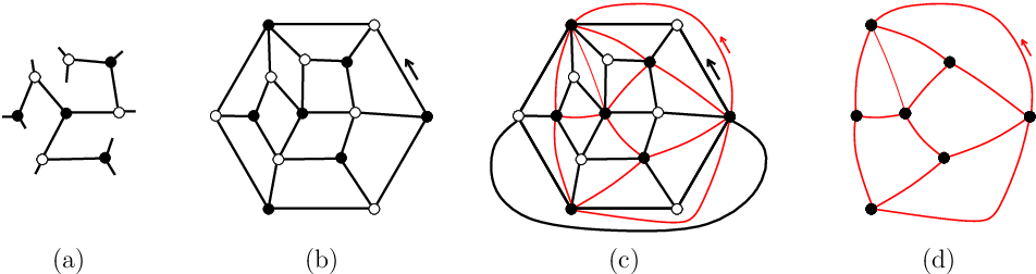
As we see next, the class $\mathcal{I}$ (and also the associated rooted class $\mathcal{J}$ ) is combinatorially tractable, as it is in bijection with the simple class of binary trees; hence irreducible dissections are easily generated at random.

4.1.4. Bijection between binary trees and irreducible dissections

There exist by now several elegant bijections between families of planar maps and families of plane trees that satisfy simple context-free decomposition grammars. Such constructions have first been described by Schaeffer in his thesis [29], and many other families of rooted maps have been counted in this way [17, 27, 28, 7]. The advantage of bijective constructions over recursive methods for counting maps [32] is that the bijections yield efficient —linear-time— generators for maps, as random sampling of maps is reduced to the much easier task of random sampling of trees, see [30]. The method has been recently applied to the family of 3-connected maps, which is of interest here. Precisely, as described in [18], there is a bijection between binary trees and irreducible dissections of the hexagon, which, as we have seen, are closely related to 3-connected maps.

We define an unrooted binary tree, shortly called a binary tree hereafter, as a plane tree (i.e., a planar map with a unique face) where the degree of each vertex is either 1 or 3. The vertices of degree 1 (3) are called leaves (nodes, resp.). A binary tree is said to be bicolored if its nodes are bicolored so that any two adjacent nodes have different colors, see Figure 6(a) for an example. In a bicolored binary tree the L-atoms are the black nodes and the U-atoms are the leaves. A bicolored binary tree is called asymmetric if there is no rotation-symmetry fixing it. Figure 7 displays the four non-asymmetric bicolored binary trees; all the other bicolored binary trees are asymmetric, either due to the shape being asymmetric, or due to the labels on the black nodes. We denote by $\mathcal{K}$ the mixed class of asymmetric bicolored binary trees (the requirement of asymmetry is necessary so that the leaves are distinguishable).

The terminology of binary tree refers to the fact that, upon rooting a binary tree at an arbitrary leaf, the neighbours in clockwise order around each node can be classified as a father (the neighbour closest to the root), a right son, and a left son, which corresponds to the classical definition of rooted binary trees, as considered in Example 3.3.

Proposition 11 (Fusy, Poulalhon, and Schaeffer [18]).

For $n\geq 0$ and $m\geq 2$ , there exists an explicit bijection, called the closure-mapping, between bicolored binary trees with $n$ black nodes and $m$ leaves, and bicolored irreducible dissections with $n$ black inner nodes and $m$ inner faces; moreover the 4 non-asymmetric bicolored binary trees are mapped to the 4 non-asymmetric irreducible dissections. In other words, the closure-mapping realises the combinatorial isomorphism

(8)

\mathcal{K}\simeq\mathcal{I}.

The construction of a dissection from a binary tree takes linear time.

Let us comment a bit on this bijective construction, which is described in detail in [18]. Starting from a binary tree, the closure-mapping builds the dissection face by face, each leaf of the tree giving rise to an inner face of the dissection. More precisely, at each step, a “leg” (i.e., an edge incident to a leaf) is completed into an edge connecting two nodes, so as to “close” a quadrangular face. At the end, an hexagon is created outside of the figure, and the leaves attached to the remaining non-completed legs are merged with vertices of the hexagon so as to form only quadrangular faces. For instance the dissection of Figure 6(b) is obtained by “closing” the tree of Figure 6(a).

4.1.5. Boltzmann sampler for rooted bicolored binary trees

We define a rooted bicolored binary tree as a binary tree with a marked leaf discarded from the set of U-atoms. Notice that the class of rooted bicolored binary trees such that the underlying unrooted binary tree is asymmetric is the U-derived class $\underline{\mathcal{K}}$ .

In order to write down a decomposition grammar for the class $\underline{\mathcal{K}}$ —to be translated into a Boltzmann sampler—we define some refined classes of rooted bicolored binary trees (decomposing $\underline{\mathcal{K}}$ is a bit involved since we have to forbid the 4 non-asymmetric binary trees): $\mathcal{R}_{\bullet}$ is the class of black-rooted binary trees (the root leaf is connected to a black node) with at least one node, and $\mathcal{R}_{\circ}$ is the class of white-rooted binary trees (the root leaf is connected to a white node) with at least one node. We also define $\mathcal{R}_{\bullet}^{\mathrm{(as)}}$ ( $\mathcal{R}_{\circ}^{\mathrm{(as)}}$ ) as the class of black-rooted (white-rooted, resp.) bicolored binary trees such that the underlying unrooted binary tree is asymmetric. Hence $\underline{\mathcal{K}}=\mathcal{R}_{\bullet}^{\mathrm{(as)}}+\mathcal{R}_{\circ}^{\mathrm{(as)}}$ . We introduce two auxiliary classes; $\widehat{\mathcal{R}}_{\bullet}$ is the class of black-rooted binary trees except the (unique) one with one black node and two white nodes; and $\widehat{\mathcal{R}}_{\circ}$ is the class of white-rooted binary trees except the two ones resulting from rooting the (unique) bicolored binary tree with one black node and three white nodes (the 4th one in Figure 7(a)), in addition, the rooted bicolored binary tree with two leaves (the first one in Figure 7(a)) is also included in the class $\widehat{\mathcal{R}}_{\circ}$ .

The decomposition of a bicolored binary tree at the root yields a complete decomposition grammar, given in Figure 8, for the class $\underline{\mathcal{K}}=\mathcal{R}_{\bullet}^{\mathrm{(as)}}+\mathcal{R}_{\circ}^{\mathrm{(as)}}$ . This grammar translates to a decomposition grammar involving only the basic classes $\{\mathcal{Z}_{L},\mathcal{Z}_{U}\}$ and the constructions $\{+,\star\}$ ( $\mathcal{Z}_{L}$ stands for a black node and $\mathcal{Z}_{U}$ stands for a non-root leaf):

(9)

\left\{\begin{array}[]{rcl}\underline{\mathcal{K}}&=&\mathcal{R}_{\bullet}^{\mathrm{(as)}}+\mathcal{R}_{\circ}^{\mathrm{(as)}},\\ \mathcal{R}_{\bullet}^{\mathrm{(as)}}&=&\mathcal{R}_{\circ}\star\mathcal{Z}_{L}\star\mathcal{Z}_{U}+\mathcal{Z}_{U}\star\mathcal{Z}_{L}\star\mathcal{R}_{\circ}+\mathcal{Z}_{L}\star\mathcal{R}_{\circ}^{2},\\ \mathcal{R}_{\circ}^{\mathrm{(as)}}&=&\widehat{\mathcal{R}}_{\bullet}\star\mathcal{Z}_{U}+\mathcal{Z}_{U}\star\widehat{\mathcal{R}}_{\bullet}+\mathcal{R}_{\bullet}^{2},\\ \widehat{\mathcal{R}}_{\bullet}&=&\widehat{\mathcal{R}}_{\circ}\star\mathcal{Z}_{L}\star\mathcal{Z}_{U}^{2}+\mathcal{Z}_{U}^{2}\star\mathcal{Z}_{L}\star\widehat{\mathcal{R}}_{\circ}+\widehat{\mathcal{R}}_{\circ}\star\mathcal{Z}_{L}\star\widehat{\mathcal{R}}_{\circ},\\ \widehat{\mathcal{R}}_{\circ}&=&\mathcal{Z}_{U}+\mathcal{R}_{\bullet}\star\mathcal{Z}_{U}+\mathcal{Z}_{U}\star\mathcal{R}_{\bullet}+\mathcal{R}_{\bullet}^{2},\\ \mathcal{R}_{\bullet}&=&(\mathcal{Z}_{U}+\mathcal{R}_{\circ})\star\mathcal{Z}_{L}\star(\mathcal{Z}_{U}+\mathcal{R}_{\circ}),\\ \mathcal{R}_{\circ}&=&(\mathcal{Z}_{U}+\mathcal{R}_{\bullet})\star(\mathcal{Z}_{U}+\mathcal{R}_{\bullet}).\end{array}\right.

In turn, this grammar is translated into a Boltzmann sampler $\Gamma\underline{\mathcal{K}}(z,w)$ for the class $\underline{\mathcal{K}}$ using the sampling rules given in Figure 3, similarly as we have done for the (simpler) class of complete binary trees in Example 1.

4.1.6. Boltzmann sampler for bicolored binary trees

We describe in this section a Boltzmann sampler $\Gamma\mathcal{K}(z,w)$ for asymmetric bicolored binary trees, which is derived from the Boltzmann sampler $\Gamma\underline{\mathcal{K}}(x,y)$ described in the previous section. Observe that each asymmetric binary tree in $\mathcal{K}_{n,m}$ gives rise to $m$ rooted binary trees in $\underline{\mathcal{K}}_{n,m-1}$ , as each of the $m$ leaves, which are distinguishable, might be chosen to be discarded from the set of U-atoms. Hence, each object of $\mathcal{K}_{n,m}$ has probability $\underline{K}(z,w)^{-1}mz^{n}/n!y^{m-1}$ to be chosen when calling $\Gamma\underline{\mathcal{K}}(z,w)$ and taking the distinguished atom back into the set of U-atoms. Hence, from the rejection lemma (Lemma 5), the sampler

repeat $\gamma\leftarrow\Gamma\underline{\mathcal{K}}(z,w)$ ;
take the distinguished U-atom back into the set of U-atoms;
{so $\|\|\gamma\|\|$ increases by $1$ and now $\gamma\in\mathcal{K}$ }
until $\mathrm{Bern}\left(\frac{2}{\|\|\gamma\|\|}\right)$ ;
return $\gamma$

is a Boltzmann sampler for $\mathcal{K}$ .

However, this sampler is not efficient enough, as it uses a massive amount of rejection to draw a tree of large size. Instead, we use an early-abort rejection algorithm, which allows us to “simulate” the rejection step all along the generation, thus making it possible to reject before the entire object is generated. We find it more convenient to use the number of nodes, instead of leaves, as the parameter for rejection (the subtle advantage is that the generation process $\Gamma\underline{\mathcal{K}}(z,w)$ builds the tree node by node). Notice that the number of leaves in an unrooted binary tree $\gamma$ is equal to $2+N(\gamma)$ , with $N(\gamma)$ the number of nodes of $\gamma$ . Hence, the rejection step in the sampler above can be replaced by a Bernoulli choice with parameter $2/(N(\gamma)+2)$ . We now give the early-abort algorithm, which repeats calling $\Gamma\underline{\mathcal{K}}(z,w)$ while using a global counter $N$ that records the number of nodes of the tree under construction.

$\Gamma\mathcal{K}(z,w)$ : repeat $N:=0$ ; {counter for nodes} Call $\Gamma\underline{\mathcal{K}}(z,w)$ each time a node is built do $N:=N+1$ ; if $\mathrm{Bern}((N+1)/(N+2))$ continue; otherwise reject and restart from the first line; od until the generation finishes; return the object generated by $\Gamma\underline{\mathcal{K}}(z,w)$ (taking the distinguished leaf back into the set of U-atoms)

Lemma 12.

The algorithm $\Gamma\mathcal{K}(z,w)$ is a Boltzmann sampler for the class $\mathcal{K}$ of asymmetric bicolored binary trees.

Proof.

At each attempt, the call to $\Gamma\underline{\mathcal{K}}(z,w)$ would output a rooted binary tree $\gamma$ if there was no early interruption. Clearly, the probability that the generation of $\gamma$ finishes without interruption is $\prod_{i=1}^{N(\gamma)}(i+1)/(i+2)=2/(N(\gamma)+2)$ . Hence, each attempt is equivalent to doing

$\gamma\leftarrow\Gamma\underline{\mathcal{K}}(z,w)$ ; if $\mathrm{Bern}\left(\frac{2}{N(\gamma)+2}\right)$ return $\gamma$ else reject;

Thus, the algorithm $\Gamma\mathcal{K}(z,w)$ is equivalent to the algorithm given in the discussion preceding Lemma 12, hence $\Gamma\mathcal{K}(z,w)$ is a Boltzmann sampler for the family $\mathcal{K}$ . ∎

4.1.7. Boltzmann sampler for irreducible dissections

As stated in Proposition 11, the closure-mapping realises a combinatorial isomorphism between asymmetric bicolored binary trees (class $\mathcal{K}$ ) and asymmetric bicolored irreducible dissections (class $\mathcal{I}$ ). Hence, the algorithm

$\Gamma\mathcal{I}(z,w)$ : $\tau\leftarrow\Gamma\mathcal{K}(z,w)$ ; return $\mathrm{closure}(\tau)$

is a Boltzmann sampler for $\mathcal{I}$ . In turn this easily yields a Boltzmann sampler for the corresponding rooted class $\mathcal{J}$ . Precisely, starting from an asymmetric bicolored irreducible dissection, each of the 3 outer black vertices, which are distinguishable, might be chosen as the root-vertex in order to obtain a rooted irreducible dissection. Moreover the sets of L-atoms and U-atoms are slightly different for the classes $\mathcal{I}$ and $\mathcal{J}$ ; indeed, a rooted dissection has one more L-atom (the black vertex following the root-vertex in cw order around the outer face) and one more U-atom (all faces are U-atoms in $\mathcal{J}$ , whereas only the inner faces are U-atoms in $\mathcal{I}$ )⁴⁴ 4 We have chosen to specify the sets of L-atoms and U-atoms in this way in order to state the isomorphisms $\mathcal{K}\simeq\mathcal{I}$ and $\mathcal{J}_{\mathrm{a}}\simeq\overrightarrow{\mathcal{M}_{3}}$ .. This yields the identity

(10)

\mathcal{J}=3\star\mathcal{Z}_{L}\star\mathcal{Z}_{U}\star\mathcal{I},

which directly yields (by the sampling rules of Figure 3) a Boltzmann sampler $\Gamma\mathcal{J}(z,w)$ for $\mathcal{J}$ from the Boltzmann sampler $\Gamma\mathcal{I}(z,w)$ .

Finally, we obtain a Boltzmann sampler for rooted admissible dissections by a simple rejection procedure

$\Gamma\mathcal{J}_{\mathrm{a}}(z,w)$ : repeat $\delta\leftarrow\Gamma\mathcal{J}(z,w)$ until $\delta\in\mathcal{J}_{\mathrm{a}}$ ; return $\delta$

4.1.8. Boltzmann sampler for rooted 3-connected maps

The Boltzmann sampler for rooted irreducible dissections and the primal-map construction yield the following sampler for rooted 3-connected maps:

$\Gamma\overrightarrow{\mathcal{M}_{3}}(z,w)$ : $\delta\leftarrow\Gamma\mathcal{J}_{\mathrm{a}}(z,w)$ ; return $\mathrm{Primal}(\delta)$

where $\mathrm{Primal}(\delta)$ is the rooted 3-connected map associated to $\delta$ (see Section 4.1.3).

4.1.9. Boltzmann sampler for edge-rooted 3-connected planar graphs

To conclude, the Boltzmann sampler $\Gamma\overrightarrow{\mathcal{M}_{3}}(z,w)$ yields a Boltzmann sampler $\Gamma\overrightarrow{\mathcal{G}_{3}}(z,w)$ for edge-rooted 3-connected planar graphs, according to the isomorphism (Whitney’s theorem) $\overrightarrow{\mathcal{M}_{3}}\simeq 2\star\overrightarrow{\mathcal{G}_{3}}$ ,

$\Gamma\overrightarrow{\mathcal{G}_{3}}(z,w)$ : return $\Gamma\overrightarrow{\mathcal{M}_{3}}(z,w)$ (forgetting the embedding)

4.2. Boltzmann sampler for 2-connected planar graphs

The next step is to realise a Boltzmann sampler for 2-connected planar graphs from the Boltzmann sampler for edge-rooted 3-connected planar graphs obtained in Section 4.1. Precisely, we first describe a Boltzmann sampler for the class $\overrightarrow{\mathcal{G}_{2}}$ of edge-rooted 2-connected planar graphs, and subsequently obtain, by using rejection techniques, a Boltzmann sampler for the class $\mathcal{G}_{2}\ \!\!\!^{\prime}$ of derived 2-connected planar graphs (having a Boltzmann sampler for $\mathcal{G}_{2}\ \!\!\!^{\prime}$ allows us to go subsequently to connected planar graphs).

To generate edge-rooted 2-connected planar graphs, we use a well-known decomposition, due to Trakhtenbrot [31], which ensures that an edge-rooted 2-connected planar graph can be assembled from edge-rooted 3-connected planar components. This decomposition deals with so-called networks (following the terminology of Walsh [34]), where a network is defined as a connected graph $N$ with two distinguished vertices $0$ and $\infty$ called poles, such that the graph $N^{*}$ obtained by adding an edge between $0$ and $\infty$ is a 2-connected planar graph. Accordingly, we refer to Trakhtenbrot’s decomposition as the network decomposition. Notice that networks are closely related to edge-rooted 2-connected planar graphs, though not completely equivalent (see Equation (11) below for the precise relation).

We rely on [34] for the description of the network decomposition. A series-network or $s$ -network is a network made of at least 2 networks connected in chain at their poles, the $\infty$ -pole of a network coinciding with the $0$ -pole of the following network in the chain. A parallel network or $p$ -network is a network made of at least 2 networks connected in parallel, so that their respective $\infty$ -poles and $0$ -poles coincide. A pseudo-brick is a network $N$ whose poles are not adjacent and such that $N^{*}$ is a 3-connected planar graph with at least 4 vertices. A polyhedral network or $h$ -network is a network obtained by taking a pseudo-brick and substituting each edge $e$ of the pseudo-brick by a network $N_{e}$ (polyhedral networks establish a link between 2-connected and 3-connected planar graphs).

Proposition 13 (Trakhtenbrot).

Networks with at least 2 edges are partitioned into $s$ -networks, $p$ -networks and $h$ -networks.

Let us explain how to obtain a recursive decomposition involving the different families of networks. (We simply adapt the decomposition formalised by Walsh [34] so as to have only positive signs.) Let $\mathcal{D}$ , $\mathcal{S}$ , $\mathcal{P}$ , and $\mathcal{H}$ be respectively the classes of networks, $s$ -networks, $p$ -networks, and $h$ -networks, where the L-atoms are the vertices except the two poles, and the U-atoms are the edges. In particular, $\mathcal{Z}_{U}$ stands here for the class containing the link-graph as only object, i.e., the graph with one edge connecting the two poles. Proposition 13 ensures that

\mathcal{D}=\mathcal{Z}_{U}+\mathcal{S}+\mathcal{P}+\mathcal{H}.

An $s$ -network can be uniquely decomposed into a non- $s$ -network (the head of the chain) followed by a network (the trail of the chain), which yields

\mathcal{S}=(\mathcal{Z}_{U}+\mathcal{P}+\mathcal{H})\star\mathcal{Z}_{L}\star\mathcal{D}.

A $p$ -network has a unique maximal parallel decomposition into a collection of at least two components that are not $p$ -networks. Observe that we consider here graphs without multiple edges, so that at most one of these components is an edge. Whether there is one or no such edge-component yields

\mathcal{P}=\mathcal{Z}_{U}\star\Set_{\geq 1}(\mathcal{S}+\mathcal{H})+\Set_{\geq 2}(\mathcal{S}+\mathcal{H}).

By definition, the class of $h$ -networks corresponds to a U-substitution of networks in pseudo-bricks; and pseudo-bricks are exactly edge-rooted 3-connected planar graphs. As a consequence (recall that $\mathcal{G}_{3}$ stands for the family of 3-connected planar graphs),

\mathcal{H}=\overrightarrow{\mathcal{G}_{3}}\circ_{U}\mathcal{D}.

To sum up, we have the following grammar corresponding to the decomposition of networks into edge-rooted 3-connected planar graphs:

Using the sampling rules (Figure 3), the decomposition grammar (N) is directly translated into a Boltzmann sampler $\Gamma\mathcal{D}(z,y)$ for networks, as given in Figure 9. A network generated by $\Gamma\mathcal{D}(z,y)$ is made of a series-parallel backbone $\beta$ (resulting from the branching structures of the calls to $\Gamma\mathcal{S}(z,y)$ and $\Gamma\mathcal{P}(z,y)$ ) and a collection of rooted 3-connected planar graphs that are attached at edges of $\beta$ ; clearly all these 3-connected components are obtained from independent calls to the Boltzmann sampler $\Gamma\overrightarrow{\mathcal{G}_{3}}(z,w)$ , with $w=D(z,y)$ .

$\Gamma\mathcal{D}(z,y)$ : Call $\Gamma\mathcal{Z}_{U}(z,y)$ or $\Gamma\mathcal{S}(z,y)$ or $\Gamma\mathcal{P}(z,y)$ or $\Gamma\mathcal{H}(z,y)$ with respective probabilities $\frac{y}{D}$ , $\frac{S}{D}$ , $\frac{P}{D}$ , $\frac{H}{D}$ ; return the network generated $\Gamma\mathcal{Z}_{U}(z,y)$ : return the link-graph $\Gamma\mathcal{S}(z,y)$ : $\gamma_{1}\leftarrow\Gamma(\mathcal{Z}_{U}+\mathcal{P}+\mathcal{H})(z,y)$ ; $\gamma_{2}\leftarrow\Gamma\mathcal{D}(z,y)$ ; $\gamma\leftarrow\gamma_{1}$ in series with $\gamma_{2}$ ; return $\gamma$ $\Gamma\mathcal{P}(z,y)$ : Call $\Gamma\mathcal{P}_{1}(z,y)$ or $\Gamma\mathcal{P}_{2}(z,y)$ with resp. probabilities $\frac{y\exp_{\geq 1}(S+H)}{P}$ , $\frac{\exp_{\geq 2}(S+H)}{P}$ ; return the network generated $\Gamma\mathcal{P}_{1}(z,y)$ : $k\leftarrow\Pois_{\geq 1}(S+H)$ ; $\gamma_{1}\leftarrow\Gamma(\mathcal{S}+\mathcal{H})(z,w),\ldots,\gamma_{k}\leftarrow\Gamma(\mathcal{S}+\mathcal{H})(z,w)$ ; {ind. calls} $\gamma\leftarrow(\gamma_{1},\ldots,\gamma_{k})$ in parallel; add to $\gamma$ an edge connecting the 2 poles; return $\gamma$ $\Gamma\mathcal{P}_{2}(z,y)$ : $k\leftarrow\Pois_{\geq 2}(S+H)$ ; $\gamma_{1}\leftarrow\Gamma(\mathcal{S}+\mathcal{H})(z,w),\ldots,\gamma_{k}\leftarrow\Gamma(\mathcal{S}+\mathcal{H})(z,w)$ ; {ind. calls} $\gamma\leftarrow(\gamma_{1},\ldots,\gamma_{k})$ in parallel; return $\gamma$ $\Gamma\mathcal{H}(z,y)$ : $\gamma\leftarrow\Gamma\overrightarrow{\mathcal{G}_{3}}(z,w)$ , with $w=D(z,y)$ ; for each edge $e$ of $\gamma$ do $\gamma_{e}\leftarrow\Gamma\mathcal{D}(z,y)$ ; substitute $e$ by $\gamma_{e}$ ; {the poles of $\gamma_{e}$ are identified with the ends of $e$ in a canonical way} od; return $\gamma$ $\Gamma(\mathcal{S}+\mathcal{H})(z,y)$ : Call $\Gamma\mathcal{S}(z,y)$ or $\Gamma\mathcal{H}(z,y)$ with resp. probabilities $\frac{S}{S+H}$ , $\frac{H}{S+H}$ ; return the network generated $\Gamma(\mathcal{Z}_{U}\!+\!\mathcal{P}\!+\!\mathcal{H})(z,y)$ : Call $\Gamma\mathcal{Z}_{U}(z,y)$ or $\Gamma\mathcal{P}(z,y)$ or $\Gamma\mathcal{H}(z,y)$ with resp. probabilities $\frac{y}{y+P+H}$ , $\frac{P}{y+P+H}$ , $\frac{H}{y+P+H}$ ; return the network generated

Figure 9. Boltzmann samplers for networks. All generating functions are assumed to be evaluated at

(z,y)

, i.e.,

D:=D(z,y)

S:=S(z,y)

P:=P(z,y)

, and

H:=H(z,y)

The only terminal nodes of the decomposition grammar are the classes $\mathcal{Z}_{L}$ , $\mathcal{Z}_{U}$ (which are explicit), and the class $\overrightarrow{\mathcal{G}_{3}}$ . Thus, the sampler $\Gamma\mathcal{D}(z,y)$ and the auxiliary samplers $\Gamma\mathcal{S}(z,y)$ , $\Gamma\mathcal{P}(z,y)$ , and $\Gamma\mathcal{H}(z,y)$ are recursively specified in terms of $\Gamma\overrightarrow{\mathcal{G}_{3}}(z,w)$ , where $w$ and $z$ are linked by $w=D(z,y)$ .

Observe that each edge-rooted 2-connected planar graph different from the link-graph gives rise to two networks, obtained respectively by keeping or deleting the root-edge. This yields the identity

(11)

(1+\mathcal{Z}_{U})\star\overrightarrow{\mathcal{G}_{2}}=(1+\mathcal{D}).

From that point, a Boltzmann sampler is easily obtained for the family $\overrightarrow{\mathcal{G}_{2}}$ of edge-rooted 2-connected planar graphs. Define a procedure AddRootEdge that adds an edge connecting the two poles $0$ and $\infty$ of a network if they are not already adjacent, and roots the obtained graph at the edge $(0,\infty)$ directed from $0$ to $\infty$ . The following sampler for $\overrightarrow{\mathcal{G}_{2}}$ is the counterpart of Equation (11).

$\Gamma(1+\mathcal{D})(z,y)$ : if $\mathrm{Bern}\left(\frac{1}{1+D(z,y)}\right)$ return the link-graph else return $\Gamma\mathcal{D}(z,y)$ ; $\Gamma\overrightarrow{\mathcal{G}_{2}}(z,y)$ : $\gamma\leftarrow\Gamma(1+\mathcal{D})(z,y)$ ; AddRootEdge( $\gamma$ ); return $\gamma$

Lemma 14.

The algorithm $\Gamma\overrightarrow{\mathcal{G}_{2}}(z,y)$ is a Boltzmann sampler for the class $\overrightarrow{\mathcal{G}_{2}}$ of edge-rooted 2-connected planar graphs.

Proof.

Firstly, observe that $\Gamma\overrightarrow{\mathcal{G}_{2}}(z,y)$ outputs the link-graph either if the initial Bernoulli choice $X$ is 0, or if $X=1$ and the sampler $\Gamma\mathcal{D}(z,y)$ picks up the link-graph. Hence the link-graph is returned with probability $(1+y)/(1+D(z,y))$ , i.e., with probability $1/\overrightarrow{G_{2}}(z,y)$ .

Apart from the link-graph, each graph $\gamma\in\overrightarrow{\mathcal{G}_{2}}$ appears twice in the class $\mathcal{E}:=1+\mathcal{D}$ : once in $\mathcal{E}_{|\gamma|,||\gamma||+1}$ (keeping the root-edge) and once in $\mathcal{E}_{|\gamma|,||\gamma||}$ (deleting the root-edge). Therefore, $\gamma$ has probability $E(z,y)^{-1}z^{|\gamma|}/|\gamma|!(y^{||\gamma||+1}+y^{||\gamma||})$ of being drawn by $\Gamma\overrightarrow{\mathcal{G}_{2}}(z,y)$ , where $E(z,y)=1+D(z,y)$ is the series of $\mathcal{E}$ . This probability simplifies to $z^{|\gamma|}/|\gamma|!y^{||\gamma||}/\overrightarrow{G_{2}}(z,y)$ . Hence, $\Gamma\overrightarrow{\mathcal{G}_{2}}(z,y)$ is a Boltzmann sampler for the class $\overrightarrow{\mathcal{G}_{2}}$ . ∎

The last step is to obtain a Boltzmann sampler for derived 2-connected planar graphs (i.e., with a distinguished vertex that is not labelled and does not count for the L-size) from the Boltzmann sampler for edge-rooted 2-connected planar graphs (as we will see in Section 4.3, derived 2-connected planar graphs constitute the blocks to construct connected planar graphs).

We proceed in two steps. Firstly, we obtain a Boltzmann sampler for the U-derived class $\underline{\mathcal{G}_{2}}$ (i.e., with a distinguished undirected edge that does not count in the U-size). Note that $\mathcal{F}:=2\star\underline{\mathcal{G}_{2}}$ satisfies $\mathcal{F}=\mathcal{Z}_{L}\ \!\!\!^{2}\star\overrightarrow{\mathcal{G}_{2}}$ . Hence, $\Gamma\overrightarrow{\mathcal{G}_{2}}(z,y)$ directly yields a Boltzmann sampler $\Gamma\mathcal{F}(z,y)$ (see the sampling rules in Figure 3). Since $\mathcal{F}=2\star\underline{\mathcal{G}_{2}}$ , a Boltzmann sampler for $\underline{\mathcal{G}_{2}}$ is obtained by calling $\Gamma\mathcal{F}(z,y)$ and then forgetting the direction of the root.

Secondly, once we have a Boltzmann sampler $\Gamma\underline{\mathcal{G}_{2}}(z,y)$ for the U-derived class $\underline{\mathcal{G}_{2}}$ , we just have to apply the procedure Uderived $\rightarrow$ Lderived (described in Section 3.4.3) to the class $\mathcal{G}_{2}$ in order to obtain a Boltzmann sampler $\Gamma\mathcal{G}_{2}\ \!\!\!^{\prime}(z,y)$ for the L-derived class $\mathcal{G}_{2}\ \!\!\!^{\prime}$ . The procedure Uderived $\rightarrow$ Lderived can be successfully applied, because the ratio vertices/edges is bounded. Indeed, each connected graph $\gamma$ satisfies $|\gamma|\leq||\gamma||+1$ , which easily yields $\alpha_{L/U}=2$ for the class $\mathcal{G}_{2}$ (attained by the link-graph).

4.3. Boltzmann sampler for connected planar graphs

Another well known graph decomposition, called the block-decomposition, ensures that a connected graph can be decomposed into 2-connected components. We take advantage of this decomposition in order to specify a Boltzmann sampler for derived connected planar graphs from the Boltzmann sampler for derived 2-connected planar graphs obtained in the last section. Then, a further rejection step yields a Boltzmann sampler for connected planar graphs.

The block-decomposition (see [21, p.10] for a detailed description) ensures that each derived connected planar graph can be uniquely constructed in the following way: take a set of derived 2-connected planar graphs and attach them together, by merging their marked vertices into a unique marked vertex. Then, for each unmarked vertex $v$ of each 2-connected component, take a derived connected planar graph $\gamma_{v}$ and merge the marked vertex of $\gamma_{v}$ with $v$ (this operation corresponds to an L-substitution). The block-decomposition gives rise to the following identity relating the classes $\mathcal{G}_{1}\ \!\!\!^{\prime}$ and $\mathcal{G}_{2}\ \!\!\!^{\prime}$ :

(12)

\mathcal{G}_{1}\ \!\!\!^{\prime}=\Set\left(\mathcal{G}_{2}\ \!\!\!^{\prime}\circ_{L}(\mathcal{Z}_{L}\star\mathcal{G}_{1}\ \!\!\!^{\prime})\right).

This is directly translated into the following Boltzmann sampler for $\mathcal{G}_{1}\ \!\!\!^{\prime}$ using the sampling rules of Figure 3. (Notice that the 2-connected blocks of a connected graph are built independently, each block resulting from a call to the Boltzmann sampler $\Gamma\mathcal{G}_{2}\ \!\!\!^{\prime}(z,y)$ , where $z=xG_{1}\ \!\!\!^{\prime}(x,y)$ .)

$\Gamma\mathcal{G}_{1}\ \!\!\!^{\prime}(x,y)$ : $k\leftarrow\Pois(G_{2}\ \!\!\!^{\prime}(z,y));\ \ [\mathrm{with}\ z=xG_{1}\ \!\!\!^{\prime}(x,y)]$ $\gamma\leftarrow(\Gamma\mathcal{G}_{2}\ \!\!\!^{\prime}(z,y),\ldots,\Gamma\mathcal{G}_{2}\ \!\!\!^{\prime}(z,y))$ ; { $k$ independent calls} merge the $k$ components of $\gamma$ at their marked vertices; for each unmarked vertex $v$ of $\gamma$ do $\gamma_{v}\leftarrow\Gamma\mathcal{G}_{1}\ \!\!\!^{\prime}(x,y)$ ; merge the marked vertex of $\gamma_{v}$ with $v$ od; return $\gamma$ .

Then, a Boltzmann sampler for connected planar graphs is simply obtained from $\Gamma\mathcal{G}_{1}\ \!\!\!^{\prime}(x,y)$ by using a rejection step so as to adjust the probability distribution:

$\Gamma\mathcal{G}_{1}(x,y)$ : repeat $\gamma\leftarrow\Gamma\mathcal{G}_{1}\ \!\!\!^{\prime}(x,y)$ 1 take the marked vertex $v$ back to the set of L-atoms; 1 (if we consider the labels, $v$ receives label $|\gamma|+1$ ) 1 {this makes $|\gamma|$ increase by $1$ , and $\gamma\in\mathcal{G}_{1}$ } until $\displaystyle\mathrm{Bern}\left(\frac{1}{|\gamma|}\right)$ ; return $\gamma$

Lemma 15.

The sampler $\Gamma\mathcal{G}_{1}(x,y)$ is a Boltzmann sampler for connected planar graphs.

Proof.

The proof is similar to the proof of Lemma 6. Due to the general property that $\mathcal{C}_{n,m}$ identifies to $\mathcal{C}^{\prime}_{n-1,m}$ , the sampler delimited inside the repeat/until loop draws each object $\gamma\in\mathcal{G}_{1}$ with probability $G_{1}\ \!\!\!^{\prime}(x,y)^{-1}\frac{x^{|\gamma|-1}}{(|\gamma|-1)!}y^{||\gamma||}$ , i.e., with probability proportional to $|\gamma|\frac{x^{|\gamma|}}{|\gamma|!}y^{||\gamma||}$ . Hence, according to Lemma 5, the sampler $\Gamma\mathcal{G}_{1}(x,w)$ draws each object $\gamma\in\mathcal{G}_{1}$ with probability proportional to $\frac{x^{|\gamma|}}{|\gamma|!}y^{||\gamma||}$ , i.e., is a Boltzmann sampler for $\mathcal{G}_{1}$ . ∎

4.4. Boltzmann sampler for planar graphs

A planar graph is classically decomposed into the set of its connected components, yielding

(13)

\mathcal{G}=\Set(\mathcal{G}_{1}),

which translates to the following Boltzmann sampler for the class $\mathcal{G}$ of planar graphs (the Set construction gives rise to a Poisson law, see Figure 3):

$\Gamma\mathcal{G}(x,y)$ : $k\leftarrow\Pois(G_{1}(x,y))$ ; return $(\Gamma\mathcal{G}_{1}(x,y),\ldots,\Gamma\mathcal{G}_{1}(x,y))$ {k independent calls}

Proposition 16.

The procedure $\Gamma\mathcal{G}(x,y)$ is a Boltzmann sampler for planar graphs.

5. Deriving an efficient sampler

We have completely described in Section 4 a mixed Boltzmann sampler $\Gamma\mathcal{G}(x,y)$ for planar graphs. This sampler yields an exact-size uniform sampler and an approximate-size uniform sampler for planar graphs: to sample at size $n$ , call the sampler $\Gamma\mathcal{G}(x,1)$ until the graph generated has size $n$ ; to sample in a range of sizes $[n(1-\epsilon),n(1+\epsilon)]$ , call the sampler $\Gamma\mathcal{G}(x,1)$ until the graph generated has size in the range. These targetted samplers can be shown to have expected polynomial complexity, of order $n^{5/2}$ for approximate-size sampling and $n^{7/2}$ for exact-size sampling (we omit the proof since we will describe more efficient samplers in this section).

However, more is needed to achieve the complexity stated in Theorem 1, i.e., $O(n/\epsilon)$ for approximate-size sampling and $O(n^{2})$ for exact-size sampling. The main problem of the sampler $\Gamma\mathcal{G}(x,1)$ is that the typical size of a graph generated is small, so that the number of attempts to reach a large target size is prohibitive.

In order to correct this effect, we design in this section a Boltzmann sampler for ‘‘bi-derived” planar graphs, which are equivalent to bi-pointed planar graphs, i.e., with 2 distinguished vertices⁵⁵ 5 In an earlier version of the article and in the conference version [16], we derived 3 times—as prescribed by [11]—in order to get a singularity type $(1-x/\rho)^{-1/2}$ (efficient targetted samplers are obtained when taking $x=\rho(1-1/(2n))$ ). We have recently discovered that deriving 2 times (which yields a square-root singularity type $(1-x/\rho)^{1/2}$ ) and taking again $x=\rho(1-1/(2n))$ yields the same complexities for the targetted samplers, with the advantage that the description and analysis is significantly simpler (in the original article [11], they prescribe to take $x=\rho$ and to use some early abort techniques for square-root singularity type, but it seems difficult to analyse the gain due to early abortion here, since the Boltzmann sampler for planar graphs makes use of rejection techniques). . The intuition is that a Boltzmann sampler for bi-pointed planar graphs gives more weight to large graphs, because a graph of size $n$ gives rise to $n(n-1)$ bi-pointed graphs. Hence, the probability of reaching a large size is better (upon choosing suitably the value of the Boltzmann parameter). The fact that the graphs have to be pointed 2 times is due to the specific asymptotic behaviour of the coefficients counting planar graphs, which has been recently analysed by Giménez and Noy [20].

5.1. Targetted samplers for classes with square-root singularities.

As we describe here, a mixed class $\mathcal{C}$ with a certain type of singularities (square-root type) gives rise to efficient approximate-size and exact-size samplers, provided $\mathcal{C}$ has a Boltzmann sampler such that the expected cost of generation is of the same order as the expected size of the object generated.

Definition 17.

Given a mixed class $\mathcal{C}$ , we define a singular point of $\mathcal{C}$ as a pair $x_{0}>0$ , $y_{0}>0$ such that the function $x\mapsto C(x,y_{0})$ has a dominant singularity at $x_{0}$ (the radius of convergence is $x_{0}$ ).

Definition 18.

For $\alpha\in\mathbb{R}\backslash\mathbb{Z}_{\geq 0}$ , a mixed class $\mathcal{C}$ is called $\alpha$ -singular if, for each singular point $(x_{0},y_{0})$ of $\mathcal{C}$ , the function $x\mapsto C(x,y_{0})$ has a unique dominant singularity at $x_{0}$ (i.e., $x_{0}$ is the unique singularity on the circle $|z|=x_{0}$ ) and admits a singular expansion of the form

C(x,y_{0})=P(x)+c_{\alpha}\cdot\left(x_{0}-x\right)^{\alpha}+o\left((x_{0}-x)^{\alpha}\right),

where $c_{\alpha}$ is a constant, $P(x)$ is rational with no poles in the disk $|z|\leq x_{0}$ , and where the expansion holds in a so-called $\Delta$ -neighbourhood of $x_{0}$ , see [14, 13]. In the special case $\alpha=1/2$ , the class is said to have square-root singularities.

Lemma 19.

Let $\mathcal{C}$ be a mixed class with square-root singularities, and endowed with a Boltzmann sampler $\Gamma\mathcal{C}(x,y)$ . Let $(x_{0},y_{0})$ be a singular point of $\mathcal{C}$ . For any $n>0$ , define

x_{n}:=\big(1-\tfrac{1}{2n}\big)\cdot x_{0}.

Call $\pi_{n}$ ( $\pi_{n,\epsilon}$ , resp.) the probability that an object $\gamma$ generated by $\Gamma\mathcal{C}(x_{n},y_{0})$ satisfies $|\gamma|=n$ ( $|\gamma|\in I_{n,\epsilon}:=[n(1-\epsilon),n(1+\epsilon)]$ , resp.); and call $\sigma_{n}$ the expected size of the output of $\Gamma\mathcal{C}(x_{n},y_{0})$ .

Then $1/\pi_{n}$ is $O(n^{3/2})$ , $1/\pi_{n,\epsilon}$ is $O(n^{1/2}/\epsilon)$ , and $\sigma_{n}$ is $O(n^{1/2})$ .

Proof.

The so-called transfer theorems of singularity analysis [13] ensure that the coefficient $a_{n}:=[x^{n}]C(x,y_{0})$ satisfies, as $n\to\infty$ , $a_{n}\mathop{\sim}_{n\to\infty}c\ \!x_{0}^{-n}n^{-3/2}$ , where $c$ is a positive constant. This easily yields the asymptotic bounds for $1/\pi_{n}$ and $1/\pi_{n,\epsilon}$ , using the expressions $\pi_{n}=a_{n}x_{n}\ \!\!\!^{n}/C(x_{n},y_{0})$ and $\pi_{n,\epsilon}=\sum_{k\in I_{n,\epsilon}}a_{k}x_{n}\ \!\!\!^{k}/C(x_{n},y_{0})$ .

It is also an easy exercise to find the asymptotics of $\sigma_{n}$ , using the formula (given in [11]) $\sigma_{n}=x_{n}\cdot\partial_{x}C(x_{n},y_{0})/C(x_{n},y_{0})$ . ∎

Lemma 19 suggests the following simple heuristic to obtain efficient targetted samplers. For approximate-size sampling (exact-size sampling, resp.), repeat calling $\Gamma\mathcal{C}(x_{n},1)$ until the size of the object is in $I_{n,\epsilon}$ (is exactly $n$ , resp.). (The parameter $y$ is useful if a target U-size $m$ is also given, as we will see for planar graphs in Section 6.2.) The complexity of sampling will be good for a class $\mathcal{C}$ that has square-root singularities and that has an efficient Boltzmann sampler. Indeed, for approximate-size sampling, the number of attempts to reach the target-domain $I_{n,\epsilon}$ (i.e., $\pi_{n,\epsilon}^{-1}$ ) is of order $n^{1/2}$ , and for exact-size sampling, the number of attempts to reach the size $n$ (i.e., $\pi_{n}^{-1}$ ) is of order $n^{3/2}$ . If $\mathcal{C}$ is endowed with a Boltzmann sampler $\Gamma\mathcal{C}(x,y)$ such that the expected complexity of sampling at $(x_{n},y_{0})$ is of order $\sqrt{n}$ (same order as the expected size $\sigma_{n}$ ), then the expected complexity is typically $O(n/\epsilon)$ for approximate-size sampling and $O(n^{2})$ for exact-size sampling, as we will see for planar graphs.

Let us mention that the original article [11] uses a different heuristic. The targetted samplers also repeat calling the Boltzmann sampler until the size of the object is in the target domain, but the parameter $x$ is chosen to be exactly at the singularity $\rho$ . The second difference is that, at each attempt, the generation is interrupted if the size of the object goes beyond the target domain. We prefer to use the simple heuristic discussed above, which does not require early interruption techniques. In this way the samplers are easier to describe and to analyse.

In order to apply these techniques to planar graphs, we have to derive two times the class of planar graphs, as indicated by the following two lemmas.

Lemma 20 ([14]).

If a class $\mathcal{C}$ is $\alpha$ -singular, then the class $\mathcal{C}^{\prime}$ is $(\alpha-1)$ -singular (by the effect of derivation).

Lemma 21 ([20]).

The class $\mathcal{G}$ of planar graphs is $5/2$ -singular, hence the class $\mathcal{G}^{\prime\prime}$ of bi-derived planar graphs has square-root singularities.

5.2. Derivation rules for Boltzmann samplers

As suggested by Lemma 19 and Lemma 21, we will get good targetted samplers for planar graphs if we can describe an efficient Boltzmann sampler for the class $\mathcal{G}^{\prime\prime}$ of bi-derived planar graphs (a graph in $\mathcal{G}^{\prime\prime}$ has two unlabelled vertices that are marked specifically, say the first one is marked $\ast$ and the second one is marked $\star$ ). Our Boltzmann sampler $\Gamma\mathcal{G}^{\prime\prime}(x,y)$ —to be presented in this section— makes use of the decomposition of planar graphs into 3-connected components which we have already successfully used to obtain a Boltzmann sampler for planar graphs in Section 4. This decomposition can be formally translated into a decomposition grammar (with additional unpointing/pointing operations). To obtain a Boltzmann sampler for bi-derived planar graphs instead of planar graphs, the idea is simply to derive this grammar 2 times.

As we explain here and as is well known in general, a decomposition grammar can be derived automatically. (In our framework, a decomposition grammar involves the 5 constructions $\{+,\star,\Set_{\geq d},\circ_{L},\circ_{U}\}$ .)

Proposition 22 (derivation rules).

The basic finite classes satisfy

(\mathbf{1})^{\prime}=0,\ \ \ (\mathcal{Z}_{L})^{\prime}=1,\ \ \ (\mathcal{Z}_{U})^{\prime}=0.

The 5 constructions satisfy the following derivation rules:

(14)

\left\{\begin{array}[]{rcl}(\mathcal{A}+\mathcal{B})^{\prime}&=&\mathcal{A}^{\prime}+\mathcal{B}^{\prime},\\ (\mathcal{A}\star\mathcal{B})^{\prime}&=&\mathcal{A}^{\prime}\star\mathcal{B}+\mathcal{A}\star\mathcal{B}^{\prime},\\ (\Set_{\geq d}(\mathcal{B}))^{\prime}&=&\mathcal{B}^{\prime}\star\Set_{\geq d-1}(\mathcal{B})\ \mathrm{for}\ d\geq 0,\ \ \ \mathrm{(with}\ \Set_{\geq-1}=\Set)\\ (\mathcal{A}\circ_{L}\mathcal{B})^{\prime}&=&\mathcal{B}^{\prime}\star(\mathcal{A}^{\prime}\circ_{L}\mathcal{B}),\\ (\mathcal{A}\circ_{U}\mathcal{B})^{\prime}&=&\mathcal{A}^{\prime}\circ_{U}\mathcal{B}+\mathcal{B}^{\prime}\star(\underline{\mathcal{A}}\circ_{U}\mathcal{B}).\end{array}\right.

Proof.

The derivation formulas for basic classes are trivial. The proof of the derivation rules for $\{+,\star,\circ_{L}\}$ are given in [3]. Notice that the rule for $\Set_{\geq d}$ follows from the rule for $\circ_{L}$ . (Indeed, $\Set_{\geq d}(\mathcal{B})=\mathcal{A}\circ_{L}\mathcal{B}$ , where $\mathcal{A}=\Set_{\geq d}(\mathcal{Z}_{L})$ , which clearly satisfies $\mathcal{A}^{\prime}=\Set_{\geq d-1}(\mathcal{Z}_{L})$ .) Finally, the proof of the rule for $\circ_{U}$ uses similar arguments as the proof of the rule for $\circ_{L}$ . In an object of $(\mathcal{A}\circ_{U}\mathcal{B})^{\prime}$ , the distinguished atom is either on the core-structure (in $\mathcal{A}$ ), or is in a certain component (in $\mathcal{B}$ ) that is substituted at a certain U-atom of the core-structure. The first case yields the term $\mathcal{A}^{\prime}\circ_{U}\mathcal{B}$ , and the second case yields the term $\mathcal{B}^{\prime}\star(\underline{\mathcal{A}}\circ_{U}\mathcal{B})$ . ∎

According to Proposition 22, it is completely automatic to find a decomposition grammar for a derived class $\mathcal{C}^{\prime}$ if we are given a decomposition grammar for $\mathcal{C}$ .

5.3. Boltzmann sampler for bi-derived planar graphs

We present in this section our Boltzmann sampler $\Gamma\mathcal{G}^{\prime\prime}(x,y)$ for bi-derived planar graphs, with a quite similar approach to the one adopted in Section 4, and again a bottom-to-top presentation. At first the closure-mapping allows us to obtain Boltzmann samplers for 3-connected planar graphs marked in various ways. Then we go from 3-connected to bi-derived planar graphs via networks, bi-derived 2-connected, and bi-derived connected planar graphs.

The complete scheme is illustrated in Figure 10, which is the counterpart of Figure 4.

5.3.1. Boltzmann samplers for derived binary trees.

We have already obtained in Section 4.1.5 a Boltzmann sampler for the class $\mathcal{K}$ of unrooted asymmetric binary trees. Our purpose here is to derive a Boltzmann sampler for the derived class $\mathcal{K}^{\prime}$ . Recall that we have also described in Section 4.1.5 a Boltzmann sampler for the U-derived class $\underline{\mathcal{K}}$ , which satisfies the completely recursive decomposition grammar (9) (see also Figure 8). Hence, we have to apply the procedure Uderived $\rightarrow$ Lderived described in Section 3.4.3 to the class $\mathcal{K}$ in order to obtain a Boltzmann sampler $\Gamma\mathcal{K}^{\prime}(z,w)$ from $\Gamma\underline{\mathcal{K}}(z,w)$ . For this we have to check that $\alpha_{L/U}$ is finite for the class $\mathcal{K}$ . It is easily proved that a bicolored binary tree with $m$ leaves has $m-2$ nodes, and that at most $\lfloor 2(m-3)/3\rfloor$ of the nodes are black. In addition, there exist trees with $3i+3$ leaves and $2i$ black nodes (those with all leaves incident to black nodes). Hence, for the class $\mathcal{K}$ , the parameter $\alpha_{L/U}$ is equal to $2/3$ . Therefore the procedure Uderived $\rightarrow$ Lderived can be applied to the class $\mathcal{K}$ .

5.3.2. Boltzmann samplers for derived rooted dissections and 3-connected maps

Our next step is to obtain Boltzmann samplers for derived irreducible dissections, in order to go subsequently to 3-connected maps. As expected we take advantage of the closure-mapping. Recall that the closure-mapping realises the isomorphism $\mathcal{K}\simeq\mathcal{I}$ between the class $\mathcal{K}$ of asymmetric binary trees and the class $\mathcal{I}$ of asymmetric irreducible dissections. There is no problem in deriving an isomorphism, so the closure-mapping also realises the isomorphism $\mathcal{K}^{\prime}\simeq\mathcal{I}^{\prime}$ . Accordingly we have the following Boltzmann sampler for the class $\mathcal{I}^{\prime}$ :

$\Gamma\mathcal{I}^{\prime}(z,w)$ : $\tau\leftarrow\Gamma\mathcal{K}^{\prime}(z,w)$ ; $\delta\leftarrow\mathrm{closure}(\tau)$ ; return $\delta$

where the discarded L-atom is the same in $\tau$ and in $\delta$ .

Then, we easily obtain a Boltzmann sampler for the corresponding rooted class $\mathcal{J}^{\prime}$ . Indeed, the equation $\mathcal{J}=3\star\mathcal{Z}_{L}\star\mathcal{Z}_{U}\star\mathcal{I}$ that relates $\mathcal{I}$ and $\mathcal{J}$ yields $\mathcal{J}^{\prime}=3\star\mathcal{Z}_{U}\star\mathcal{I}+3\star\mathcal{Z}_{L}\star\mathcal{Z}_{U}\star\mathcal{I}^{\prime}$ . Hence, using the sampling rules of Figure 3, we obtain a Boltzmann sampler $\Gamma\mathcal{J}^{\prime}(z,w)$ from the Boltzmann samplers $\Gamma\mathcal{I}(z,w)$ and $\Gamma\mathcal{I}^{\prime}(z,w)$ .

From that point, we obtain a Boltzmann sampler for the derived rooted dissections that are admissible. As $\mathcal{J}_{\mathrm{a}}\subset\mathcal{I}$ , we also have $\mathcal{J}_{\mathrm{a}}^{\prime}\subset\mathcal{J}^{\prime}$ , which yields the following Boltzmann sampler for $\mathcal{J}_{\mathrm{a}}^{\prime}$ :

$\Gamma\mathcal{J}_{\mathrm{a}}^{\prime}(z,w)$ : repeat $\delta\leftarrow\Gamma\mathcal{J}^{\prime}(z,w)$ until $\delta\in\mathcal{J}_{\mathrm{a}}^{\prime}$ ; return $\delta$

Finally, using the isomorphism $\mathcal{J}_{\mathrm{a}}\simeq\overrightarrow{\mathcal{M}_{3}}$ (primal map construction, Section 4.1.3), which yields $\mathcal{J}_{\mathrm{a}}^{\prime}\simeq\overrightarrow{\mathcal{M}_{3}}^{\prime}$ , we obtain a Boltzmann samplers for derived rooted 3-connected maps:

$\Gamma\overrightarrow{\mathcal{M}_{3}}^{\prime}(z,w)$ : $\delta\leftarrow\Gamma\mathcal{J}_{\mathrm{a}}^{\prime}(z,w)$ ; return $\mathrm{Primal}(\delta)$

where the returned rooted 3-connected map inherits the distinguished L-atom of $\delta$ .

5.3.3. Boltzmann samplers for derived rooted 3-connected planar graphs.

As we have seen in Section 4.1.2, Whitney’s theorem states that any 3-connected planar graph has two embeddings on the sphere (which differ by a reflection). Clearly the same property holds for 3-connected planar graphs that have additional marks. (We have already used this observation in Section 4.1.2 for rooted graphs, $\overrightarrow{\mathcal{M}_{3}}\simeq 2\star\overrightarrow{\mathcal{G}_{3}}$ , in order to obtain a Boltzmann sampler for $\overrightarrow{\mathcal{G}_{3}}$ .) Hence $\overrightarrow{\mathcal{M}_{3}}^{\prime}\simeq 2\star\overrightarrow{\mathcal{G}_{3}}^{\prime}$ , which yields the following Boltzmann sampler for $\overrightarrow{\mathcal{G}_{3}}^{\prime}$ :

$\Gamma\overrightarrow{\mathcal{G}_{3}}^{\prime}(z,w)$ : return $\Gamma\overrightarrow{\mathcal{M}_{3}}^{\prime}(z,w)$ ; (forgetting the embedding)

The next step (in Section 5.4) is to go to derived networks. This asks for a derivation of the decomposition grammar for networks, which involves not only the classes $\overrightarrow{\mathcal{G}_{3}}$ , $\overrightarrow{\mathcal{G}_{3}}^{\prime}$ , but also the U-derived class $\underline{\overrightarrow{\mathcal{G}_{3}}}$ . Hence, we also need a Boltzmann sampler for $\underline{\overrightarrow{\mathcal{G}_{3}}}$ .

To this aim we just have to apply the procedure Lderived $\rightarrow$ Uderived to the class $\overrightarrow{\mathcal{G}_{3}}$ . By the Euler relation, a 3-connected planar graph with $n$ vertices has at most $3n-6$ edges (equality holds for triangulations). Hence, the parameter $\alpha_{U/L}$ is equal to $3$ for the class $\overrightarrow{\mathcal{G}_{3}}$ , so Lderived $\rightarrow$ Uderived can be successfully applied to $\overrightarrow{\mathcal{G}_{3}}$ , yielding a Boltzmann sampler for $\underline{\overrightarrow{\mathcal{G}_{3}}}$ from the Boltzmann sampler for $\overrightarrow{\mathcal{G}_{3}}^{\prime}$ .

5.4. Boltzmann samplers for derived networks.

Following the general scheme shown in Figure 10, our aim is now to obtain a Boltzmann samplers for the class $\mathcal{D}^{\prime}$ of derived networks. Recall that the decomposition grammar for $\mathcal{D}$ has allowed us to obtain a Boltzmann sampler for $\mathcal{D}$ from a Boltzmann sampler for $\overrightarrow{\mathcal{G}_{3}}$ . Using the derivation rules (Proposition 22) injected in the grammar (N), we obtain the following decomposition grammar for $\mathcal{D}^{\prime}$ :

The only terminal classes in this grammar are $\overrightarrow{\mathcal{G}_{3}}^{\prime}$ and $\underline{\overrightarrow{\mathcal{G}_{3}}}$ . Hence, the sampling rules of Figure 3 yield a Boltzmann sampler for $\mathcal{D}^{\prime}$ from the Boltzmann samplers for $\overrightarrow{\mathcal{G}_{3}}^{\prime}$ and $\underline{\overrightarrow{\mathcal{G}_{3}}}$ which we have obtained in Section 5.3.3. The sampler $\Gamma\mathcal{D}^{\prime}(z,y)$ looks similar (though with more cases) to the one for $\Gamma\mathcal{D}(z,y)$ given in Figure 9.

5.5. Boltzmann samplers for bi-derived 2-connected planar graphs.

The aim of this section is to obtain Boltzmann samplers for the class $\mathcal{G}_{2}\ \!\!\!^{\prime\prime}$ of bi-derived 2-connected planar graphs (after the Boltzmann sampler for $\mathcal{G}_{2}\ \!\!\!^{\prime}$ obtained in Section 4.2), in order to go subsequently to bi-derived connected planar graphs.

At first, the Boltzmann sampler for $\mathcal{D}^{\prime}$ yields a Boltzmann sampler for the class $\overrightarrow{\mathcal{G}_{2}}^{\prime}$ . Indeed the identity $(1+\mathcal{D})=(1+\mathcal{Z}_{U})\star\overrightarrow{\mathcal{G}_{2}}$ is derived as $\mathcal{D}^{\prime}=(1+\mathcal{Z}_{U})\star\overrightarrow{\mathcal{G}_{2}}^{\prime}$ , which yields the following sampler,

$\Gamma\overrightarrow{\mathcal{G}_{2}}^{\prime}(z,y)$ : $\gamma\leftarrow\Gamma\mathcal{D}^{\prime}(z,y)$ ; $\textsc{AddRootEdge}(\gamma)$ ; return $\gamma$

where AddRootEdge has been defined in Section 4.2. The proof that this is a Boltzmann sampler for $\overrightarrow{\mathcal{G}_{2}}^{\prime}$ is similar to the proof of Lemma 14.

Next we describe a Boltzmann sampler for the class $\underline{\mathcal{G}_{2}}^{\prime}$ . As we have seen in Section 4.2, $\underline{\mathcal{G}_{2}}$ and $\overrightarrow{\mathcal{G}_{2}}$ are related by the identity $2\star\underline{\mathcal{G}_{2}}=\mathcal{Z}_{L}\ \!\!\!^{2}\star\overrightarrow{\mathcal{G}_{2}}$ . Hence, if we define $\mathcal{F}:=2\star\underline{\mathcal{G}_{2}}$ , we have $\mathcal{F}^{\prime}=\mathcal{Z}_{L}\ \!\!\!^{2}\star\overrightarrow{\mathcal{G}_{2}}^{\prime}+2\star\mathcal{Z}_{L}\star\overrightarrow{\mathcal{G}_{2}}$ . Hence, the sampling rules of Figure 3 yield a Boltzmann sampler $\Gamma\mathcal{F}^{\prime}(z,y)$ for the class $\mathcal{F}^{\prime}$ . Clearly, as $\mathcal{F}^{\prime}=2\star\underline{\mathcal{G}_{2}}^{\prime}$ , a Boltzmann sampler for $\underline{\mathcal{G}_{2}}^{\prime}$ is obtained by calling $\Gamma\mathcal{F}^{\prime}(z,y)$ and forgetting the direction of the root.

Finally, the procedure Uderived $\rightarrow$ Lderived yields (when applied to $\mathcal{G}_{2}\ \!\!\!^{\prime}$ ) from the Boltzmann sampler for $\underline{\mathcal{G}_{2}}^{\prime}$ to a Boltzmann sampler for $\mathcal{G}_{2}\ \!\!\!^{\prime\prime}$ . The procedure can be successfully applied, as the class $\mathcal{G}_{2}\ \!\!\!^{\prime}$ satisfies $\alpha_{L/U}=1$ (attained by the link-graph).

5.5.1. Boltzmann sampler for bi-derived connected planar graphs.

The block-decomposition makes it easy to obtain a Boltzmann sampler for the class $\mathcal{G}_{1}\ \!\!\!^{\prime\prime}$ of bi-derived connected planar graphs (this decomposition has already allowed us to obtain a Boltzmann sampler for $\mathcal{G}_{1}\ \!\!\!^{\prime}$ in Section 4.3). Recall that the block-decomposition yields the identity

\mathcal{G}_{1}\ \!\!\!^{\prime}=\Set\left(\mathcal{G}_{2}\ \!\!\!^{\prime}\circ_{L}(\mathcal{Z}_{L}\star\mathcal{G}_{1}\ \!\!\!^{\prime})\right),

which is derived as

\mathcal{G}_{1}\ \!\!\!^{\prime\prime}=(\mathcal{G}_{1}\ \!\!\!^{\prime}+\mathcal{Z}_{L}\star\mathcal{G}_{1}\ \!\!\!^{\prime\prime})\star\mathcal{G}_{2}\ \!\!\!^{\prime\prime}\circ_{L}(\mathcal{Z}_{L}\star\mathcal{G}_{1}\ \!\!\!^{\prime})\star\mathcal{G}_{1}\ \!\!\!^{\prime}.

As we already have Boltzmann samplers for the classes $\mathcal{G}_{2}\ \!\!\!^{\prime\prime}$ and $\mathcal{G}_{1}\ \!\!\!^{\prime}$ , the sampling rules of Figure 3 yield a Boltzmann sampler $\Gamma\mathcal{G}_{1}\ \!\!\!^{\prime\prime}(x,y)$ for the class $\mathcal{G}_{1}\ \!\!\!^{\prime\prime}$ . Observe that the 2-connected blocks of a graph generated by $\Gamma\mathcal{G}_{1}\ \!\!\!^{\prime\prime}(x,y)$ are obtained as independent calls to $\Gamma\mathcal{G}_{2}\ \!\!\!^{\prime}(z,y)$ and $\Gamma\mathcal{G}_{2}\ \!\!\!^{\prime\prime}(z,y)$ , where $z$ and $x$ are related by the change of variable $z=xG_{1}\ \!\!\!^{\prime}(x,y)$ .

5.5.2. Boltzmann samplers for bi-derived planar graphs

We can now achieve our goal, i.e., obtain a Boltzmann sampler for the class $\mathcal{G}^{\prime\prime}$ of bi-derived planar graphs. For this purpose, we simply derive twice the identity

\mathcal{G}=\Set(\mathcal{G}_{1}),

which yields successively the identities

\mathcal{G}^{\prime}=\mathcal{G}_{1}\ \!\!\!^{\prime}\star\mathcal{G},

and

\mathcal{G}^{\prime\prime}=\mathcal{G}_{1}\ \!\!\!^{\prime\prime}\star\mathcal{G}+\mathcal{G}_{1}\ \!\!\!^{\prime}\star\mathcal{G}^{\prime}.

From the first identity and $\Gamma\mathcal{G}(x,y)$ , $\Gamma\mathcal{G}_{1}\ \!\!\!^{\prime}(x,y)$ , we get a Boltzmann sampler $\Gamma\mathcal{G}^{\prime}(x,y)$ for the class $\mathcal{G}^{\prime}$ . Then, from the second identity and $\Gamma\mathcal{G}(x,y)$ , $\Gamma\mathcal{G}^{\prime}(x,y)$ , $\Gamma\mathcal{G}_{1}\ \!\!\!^{\prime}(x,y)$ , $\Gamma\mathcal{G}_{1}\ \!\!\!^{\prime\prime}(x,y)$ , we get a Boltzmann sampler $\Gamma\mathcal{G}^{\prime\prime}(x,y)$ for the class $\mathcal{G}^{\prime\prime}$ .

6. The targetted samplers for planar graphs

The Boltzmann sampler $\Gamma\mathcal{G}^{\prime\prime}(x,y)$ —when tuned as indicated in Lemma 19—yields efficient exact-size and approximate-size random samplers for planar graphs, with the complexities as stated in Theorem 1 and Theorem 2. Define the algorithm:

$\textsc{SamplePlanar}(x,y)$ :	$\gamma\leftarrow\Gamma\mathcal{G}^{\prime\prime}(x,y)$ ;
	give label $\|\gamma\|+1$ to the vertex marked $\star$
	and label $\|\gamma\|+2$ to the marked vertex $\ast$
	(thus $\|\gamma\|$ increases by $2$ , and $\gamma\in\mathcal{G}$ );
	return $\gamma$

6.1. Samplers according to the number of vertices

Let $\rho_{G}$ be the radius of convergence of $x\mapsto G(x,1)$ . Define

x_{n}:=\big(1-\tfrac{1}{2n}\big)\cdot\rho_{G}.

For $n\geq 1$ , the exact-size sampler is

$\mathfrak{A}_{n}$ : repeat $\gamma\leftarrow\textsc{SamplePlanar}(x_{n},1)$ until $|\gamma|=n$ ; return $\gamma$ .

For $n\geq 1$ and $\epsilon>0$ , the approximate-size sampler is

$\mathfrak{A}_{n,\epsilon}$ : repeat $\gamma\leftarrow\textsc{SamplePlanar}(x_{n},1)$ until $|\gamma|\in[n(1-\epsilon),n(1+\epsilon)]$ ; return $\gamma$ .

6.2. Samplers according to the numbers of vertices and edges

For any $y>0$ , we denote by $\rho_{G}(y)$ the radius of convergence of $x\mapsto G(x,y)$ . Let $\mu(y)$ be the function defined as

\mu(y):=-y\frac{\mathrm{d}\rho_{G}}{\mathrm{d}y}(y)/\rho_{G}(y).

As proved in [20] (using the so-called quasi-power theorem), for a fixed $y>0$ , a large graph drawn by the Boltzmann sampler $\Gamma\mathcal{G}^{\prime\prime}(x,y)$ has a ratio edges/vertices concentrated around the value $\mu(y)$ as $x$ approaches the radius of convergence of $x\mapsto G(x,y)$ . This yields a relation between the secondary parameter $y$ and the ratio edges/vertices. If we want a ratio edges/vertices close to a target value $\mu$ , we have to choose $y$ so that $\mu(y)=\mu$ . It is shown in [20] that the function $\mu(y)$ is strictly increasing on $(0,+\infty)$ , with $\lim\mu(y)=1$ as $y\to 0$ and $\lim\mu(y)=3$ as $y\to+\infty$ . As a consequence, $\mu(y)$ has an inverse function $y(\mu)$ defined on $(1,3)$ . (In addition, $\mu\mapsto y(\mu)$ can be evaluated with good precision from the analytic equation it satisfies.) We define

x_{n}(\mu):=\big(1-\tfrac{1}{2n}\big)\cdot\rho_{G}(y(\mu)).

For $n\geq 1$ and $\mu\in(1,3)$ , the exact-size sampler is

$\overline{\mathfrak{A}}_{n,\mu}$ : repeat $\gamma\leftarrow\textsc{SamplePlanar}(x_{n}(\mu),y(\mu))$ until ( $|\gamma|\!=\!n$ and $||\gamma||\!=\!\lfloor\mu n\rfloor)$ ; return $\gamma$ .

For $n\geq 1$ , $\mu\in(1,3)$ , and $\epsilon>0$ , the approximate-size sampler is

$\overline{\mathfrak{A}}_{n,\mu,\epsilon}$ :	repeat $\gamma\leftarrow\textsc{SamplePlanar}(x_{n}(\mu),y(\mu))$
	until ( $\|\gamma\|\in[n(1-\epsilon),n(1+\epsilon)]$ and $\frac{\|\|\gamma\|\|}{\|\gamma\|}\in[\mu(1-\epsilon),\mu(1+\epsilon)]$ );
	return $\gamma$ .

The complexity of the samplers is analysed in Section 8.

7. Implementation and experimental results

7.1. Implementation

We have completely implemented the random samplers for planar graphs described in Section 5. First we evaluated with good precision—typically 20 digits—the generating functions of the families of planar graphs that intervene in the decomposition (general, connected, 2-connected, 3-connected), derived up to 2 times. The calculations have been carried out in Maple using the analytic expressions of Giménez and Noy for the generating functions [20]. We have performed the evaluations for values of the parameter $x$ associated with a bunch of reference target sizes in logarithmic scale, $n=\{10^{2},10^{3},10^{4},10^{5},10^{6}\}$ . From the evaluations of the generating functions, we have computed the vectors of real values that are associated to the random choices to be performed during the generation, e.g., a Poisson law vector with parameter $G_{1}(x)$ (the EGF of connected planar graphs) is used for drawing the number of connected components of the graph.

The second step has been the implementation of the random sampler in Java. To build the graph all along the generation process, it proves more convenient to manipulate a data structure specific to planar maps rather than planar graphs. The advantage is also that the graph to be generated will be equipped with an explicit (arbitrary) planar embedding. Thus if the graph generated is to be drawn in the plane, we do not need to call the rather involved algorithms for embedding a planar graph. Planar maps are suitably manipulated using the so-called half-edge structure, where each half-edge occupies a memory block containing a pointer to the opposite half-edge along the same edge and to the next half-edge in ccw order around the incident vertex. Using the half-edge structure, it proves very easy to implement in cost $O(1)$ all primitives used for building the graph—typically, merging two components at a common vertex or edge. Doing this, the actual complexity of implementation corresponds to the complexity of the random samplers as stated in Theorem 1 and Theorem 2: linear for approximate-size sampling and quadratic for exact-size sampling. In practice, generating a graph of size of order $10^{5}$ takes a few seconds on a standard computer.

7.2. Experimentations.

The good complexity of our random samplers allows us to observe statistical properties of parameters on very large random planar graphs—in the range of sizes $10^{5}$ —where the asymptotic regime is already visible. We focus here on parameters that are known or expected to be concentrated around a limit value. Note that the experimentations are on connected planar graphs instead of general planar graphs. (It is slightly easier to restrict the implementation to connected graphs, which are conveniently manipulated using the half-edge data structure.) However, from the works of Giménez and Noy [20] and previous work by MacDiarmid et al. [23], a random planar graph consists of a huge connected component, plus other components whose total expected size is $O(1)$ . Thus, statistical properties like those stated in Conjecture 23 should be the same for random planar graphs as for random connected planar graphs.

Number of edges. First we have checked that the random variable $X_{n}$ that counts the number of edges in a random connected planar graph with $n$ vertices is concentrated. Precisely, Giménez and Noy have proved that $Y_{n}:=X_{n}/n$ converges in law to a constant $\mu\approx 2.213$ , (they also show that the fluctuations are gaussian of magnitude $1/\sqrt{n}$ ). Figure 11 shows in ordinate the ratio edges/vertices for a collection of 80 random connected planar graphs of size at least $10^{4}$ drawn by our sampler. As we can see, the ratios are concentrated around the horizontal line $y=\mu$ , agreeing with the convergence result of Giménez and Noy.

Degrees of vertices. Another parameter of interest is the distribution of the degrees of vertices in a random planar graph. For a planar graph $\gamma$ with $n$ vertices, we denote by $N^{(k)}(\gamma)$ the number of vertices of $\gamma$ that have $k$ neighbours. Accordingly, $Z^{(k)}(\gamma):=N^{(k)}(\gamma)/n$ is the proportion of vertices of degree $k$ in $\gamma$ . It is known from Giménez and Noy that, for $k=1,2$ , the random variable $Z^{(k)}$ converges in law to an explicit constant. Figure 12 shows in abscissa the parameter $k$ and in ordinate the value of $Z^{(k)}$ for a collection of 80 random connected planar graphs of size at least $10^{4}$ drawn by our sampler. Hence, the vertical line at abscissa $k$ is occupied by 80 points whose ordinates correspond to the values taken by $Z^{(k)}$ for each of the graphs. As we can see, for $k$ small—typically $k<<\log n$ —the values of $Z^{(k)}$ are concentrated around a constant. This leads us to the following conjecture.

Conjecture 23.

For every $k\geq 1$ , let $Z^{(k)}_{n}$ be the random variable denoting the proportion of vertices of degree $k$ in a random planar graph with $n$ vertices taken uniformly at random. Then $Z_{n}^{(k)}$ converges in law to an explicit constant $\pi^{(k)}$ as $n\to\infty$ ; and $\sum_{k}\pi^{(k)}=1$ .

Let us mention some progress on this conjecture. It has recently been proved in [10] that the expected values $\mathbb{E}(Z_{n}^{(k)})$ converge as $n\to\infty$ to constants $\pi^{(k)}$ that are computable and satisfy $\sum_{k}\pi^{(k)}=1$ . Hence, what remains to be shown regarding the conjecture is the concentration property.

8. Analysis of the time complexity

This whole section is dedicated to the proof of the complexities of the targetted random samplers. We show that the expected complexities of the targetted samplers $\mathfrak{A}_{n}$ , $\mathfrak{A}_{n,\epsilon}$ , $\overline{\mathfrak{A}}_{n,\mu}$ , and $\overline{\mathfrak{A}}_{n,\mu,\epsilon}$ , as described in Section 6, are respectively $O(n^{2})$ , $O(n/\epsilon)$ , $O_{\mu}(n^{5/2})$ , and $O_{\mu}(n/\epsilon)$ respectively (the dependency in $\mu$ in not analysed for the sake of simplicity).

Recall that the targetted samplers call $\Gamma\mathcal{G}^{\prime\prime}(x,y)$ (with suitable values of $x$ and $y$ ) until the size parameters are in the target domain. Accordingly, the complexity analysis is done in two steps. In the first step, we estimate the probability of hitting the target domain, which allows us to reduce the complexity analysis to the analysis of the expected complexity of the pure Boltzmann sampler $\Gamma\mathcal{G}^{\prime\prime}(x,y)$ . We use a specific notation to denote such an expected complexity:

Definition 24.

Given a class $\mathcal{C}$ endowed with a Boltzmann sampler $\Gamma\mathcal{C}(x,y)$ , we denote by $\Lambda\mathcal{C}(x,y)$ the expected combinatorial complexity⁶⁶ 6 See the discussion on the complexity model after the statement of Theorem 2 in the introduction. of a call to $\Gamma\mathcal{C}(x,y)$ (note that $\Lambda\mathcal{C}(x,y)$ depends not only on $\mathcal{C}$ , but also on a specific Boltzmann sampler for $\mathcal{C}$ ).

Typically the values $(x,y)$ have to be close to a singular point of $\mathcal{G}$ in order to draw graphs of large size. Hence, in the second step, our aim is to bound $\Lambda\mathcal{G}^{\prime\prime}(x,y)$ when $(x,y)$ converges to a given singular point $(x_{0},y_{0})$ of $\mathcal{G}$ . To analyse $\Lambda\mathcal{G}^{\prime\prime}(x,y)$ , our approach is again from bottom to top, as the description of the sampler in Section 5 (see also the general scheme summarized in Figure 10). At each step we give asymptotic bounds for the expected complexities of the Boltzmann samplers when the parameters approach a singular point. This study requires the knowledge of the singular behaviours of all series involved in the decomposition of bi-derived planar graphs, which are recalled in Section 8.5.

8.1. Complexity of rejection: the key lemma

The following simple lemma will be extensively used, firstly to reduce the complexity analysis of the targetted samplers to the one of pure Boltzmann samplers, secondly to estimate the effect of the rejection steps on the expected complexities of the Boltzmann samplers.

Lemma 25 (rejection complexity).

Let $\mathfrak{A}$ be a random sampler on a combinatorial class $\mathcal{C}$ according to a probability distribution $\mathbb{P}$ , and let $p:\mathcal{C}\to[0,1]$ be a function on $\mathcal{C}$ , called the rejection function. Consider the rejection algorithm

$\mathfrak{A}_{\mathrm{rej}}$ : repeat $\gamma\leftarrow\mathfrak{A}$ until $\Bern(p(\gamma))$ return $\gamma$ .

Then the expected complexity $\mathbb{E}(\mathfrak{A}_{\mathrm{rej}})$ of $\mathfrak{A}_{\mathrm{rej}}$ and the expected complexity $\mathbb{E}(\mathfrak{A})$ of $\mathfrak{A}$ are related by

(15)

\mathbb{E}(\mathfrak{A}_{\mathrm{rej}})=\frac{1}{p_{\mathrm{acc}}}\mathbb{E}(\mathfrak{A}),

where $p_{\mathrm{acc}}:=\sum_{\gamma\in\mathcal{C}}\mathbb{P}(\gamma)p(\gamma)$ is the probability of success of $\mathfrak{A}_{\mathrm{rej}}$ at each attempt.

Proof.

The quantity $\mathbb{E}(\mathfrak{A}_{\mathrm{rej}})$ satisfies the recursive equation

\mathbb{E}(\mathfrak{A}_{\mathrm{rej}})=\mathbb{E}(\mathfrak{A})+(1-p_{\mathrm{acc}})\mathbb{E}(\mathfrak{A}_{\mathrm{rej}}).

Indeed, a first attempt, with expected complexity $\mathbb{E}(\mathfrak{A})$ , is always needed; and in case of rejection, occurring with probability $(1-p_{\mathrm{acc}})$ , the sampler restarts in the same way as when it is launched. ∎

As a corollary we obtain the following useful formulas to estimate the effect of rejection in Boltzmann samplers when going from L-derived (vertex-pointed) to U-derived (edge-pointed) graphs and vice-versa.

Corollary 26 (Complexity of changing the root).

Let $\mathcal{A}$ be a mixed combinatorial class such that the constants $\alpha_{U/L}:=\mathrm{max}_{\gamma\in\mathcal{A}}\frac{||\gamma||}{|\gamma|}$ and $\alpha_{L/U}:=\mathrm{max}_{\gamma\in\mathcal{A}}\frac{|\gamma|}{||\gamma||}$ are finite. Define $c:=\alpha_{U/L}\cdot\alpha_{L/U}$ .

•

Assume $\mathcal{A}^{\prime}$ is equipped with a Boltzmann sampler, and let $\Gamma\underline{\mathcal{A}}(x,y)$ be the Boltzmann sampler for $\underline{\mathcal{A}}$ obtained by applying Lderived $\rightarrow$ Uderived ---as defined in Section 3.4.3—to $\mathcal{A}$ . Then

$\Lambda\underline{\mathcal{A}}(x,y)\leq c\cdot\Lambda\mathcal{A}^{\prime}(x,y).$
•

Assume $\underline{\mathcal{A}}$ is equipped with a Boltzmann sampler, and let $\Gamma\mathcal{A}^{\prime}(x,y)$ be the Boltzmann sampler for $\mathcal{A}^{\prime}$ obtained by applying Uderived $\rightarrow$ Lderived ---as defined in Section 3.4.3—to $\mathcal{A}$ . Then

$\Lambda\mathcal{A}^{\prime}(x,y)\leq c\cdot\Lambda\underline{\mathcal{A}}(x,y).$

Proof.

Let us give the proof for Lderived $\rightarrow$ Uderived (the other case is proved in a similar way). By definition of Lderived $\rightarrow$ Uderived the probability of the Bernoulli choice at each attempt in $\Gamma\underline{\mathcal{A}}(x,y)$ is at least $\frac{1}{\alpha_{U/L}}\mathrm{min}_{\gamma\in\mathcal{A}}\frac{||\gamma||}{|\gamma|}$ , i.e., at least $1/(\alpha_{U/L}\cdot\alpha_{L/U})$ . Hence the probability $p_{\mathrm{acc}}$ of success at each attempt is at least $1/c$ . Therefore, by Corollary 26, $\Lambda\underline{\mathcal{A}}(x,y)=\Lambda\mathcal{A}^{\prime}(x,y)/p_{\mathrm{acc}}\leq c\cdot\Lambda\mathcal{A}^{\prime}(x,y)$ . ∎

8.2. Reduction to analysing the expected complexity of Boltzmann samplers

We prove here that analysing the expected complexities of the targetted samplers reduces to analysing the expected complexity $\Lambda\mathcal{G}^{\prime\prime}(x,y)$ when $(x,y)$ approaches a singular point. (Recall that a singular point $(x_{0},y_{0})$ for a class $\mathcal{C}$ is such that the function $x\mapsto C(x,y_{0})$ has a dominant singularity at $x_{0}$ .)

Claim 27.

Assume that for every singular point $(x_{0},y_{0})$ of $\mathcal{G}$ , the expected complexity of the Boltzmann sampler for $\mathcal{G}^{\prime\prime}$ satisfies⁷⁷ 7 In this article all convergence statements are meant “from below”, i.e., $x\to x_{0}$ means that $x$ approaches $x_{0}$ while staying smaller than $x_{0}$ .

(16)

\Lambda\mathcal{G}^{\prime\prime}(x,y_{0})=O((x_{0}-x)^{-1/2})\ \ \mathrm{as}\ x\to x_{0}.

Then the expected complexities of the targetted samplers $\mathfrak{A}_{n}$ , $\mathfrak{A}_{n,\epsilon}$ , $\overline{\mathfrak{A}}_{n,\mu}$ , and $\overline{\mathfrak{A}}_{n,\mu,\epsilon}$ —as defined in Section 6—are respectively $O(n^{2})$ , $O(n/\epsilon)$ , $O_{\mu}(n^{5/2})$ , and $O_{\mu}(n/\epsilon)$ .

In other words, proving (16) is enough to prove the complexities of the random samplers for planar graphs, as stated in Theorem 1 and Theorem 2.

Proof.

Assume that (16) holds. Let $\pi_{n,\epsilon}$ ( $\pi_{n}$ , resp.) be the probability that the output of $\textsc{SamplePlanar}(x_{n},1)$ —with $x_{n}=(1-1/2n)\cdot\rho_{G}$ — has size in $I_{n,\epsilon}:=[n(1-\epsilon),n(1+\epsilon)]$ (has size $n$ , resp.). According to Lemma 25, the expected complexities of the exact-size and approximate-size samplers with respect to vertices —as described in Section 6.1— satisfy

\mathbb{E}(\mathfrak{A_{n}})=\frac{\Lambda\mathcal{G}^{\prime\prime}(x_{n},1)}{\pi_{n}},\ \ \ \ \ \ \ \mathbb{E}(\mathfrak{A_{n,\epsilon}})=\frac{\Lambda\mathcal{G}^{\prime\prime}(x_{n},1)}{\pi_{n,\epsilon}}.

Equation (16) ensures that, when $n\to\infty$ , $\Lambda\mathcal{G}^{\prime\prime}(x_{n},1)$ is $O(n^{1/2})$ . In addition, according to Lemma 21, $\mathcal{G}^{\prime\prime}$ is $1/2$ -singular (square-root singularities). Hence, by Lemma 19, $1/\pi_{n}$ is $O(n^{3/2})$ and $1/\pi_{n,\epsilon}$ is $O(n^{1/2}/\epsilon)$ . Thus, $\mathbb{E}(\mathfrak{A_{n}})$ is $O(n^{2})$ and $\mathbb{E}(\mathfrak{A_{n,\epsilon}})$ is $O(n/\epsilon)$ .

The proof for the samplers with respect to vertices and edges is a bit more technical. Consider a planar graph $\gamma$ drawn by the sampler $\textsc{SamplePlanar}(x_{n}(\mu),y(\mu))$ . In view of the proof for the exact-size sampler, define

\overline{\pi}_{n\wedge\mu}:=\mathbb{P}(||\gamma||\!=\!\lfloor\mu n\rfloor,|\gamma|=n),\ \ \overline{\pi}_{\mu|n}:=\mathbb{P}(||\gamma||\!\!=\!\!\lfloor\mu n\rfloor\ |\ |\gamma|\!\!=\!\!n),\ \ \pi_{n}:=\mathbb{P}(|\gamma|\!\!=\!\!n).

In view of the proof for the approximate-size sampler, define

\overline{\pi}_{n\wedge\mu,\epsilon}:=\mathbb{P}(|\gamma|\in[n(1-\epsilon),n(1+\epsilon)],\ ||\gamma||/|\gamma|\in[\mu(1-\epsilon),\mu(1+\epsilon)]),

\overline{\pi}_{\mu|n,\epsilon}:=\mathbb{P}(||\gamma||/|\gamma|\in[\mu(1-\epsilon),\mu(1+\epsilon)]\ |\ |\gamma|\in[n(1-\epsilon),n(1+\epsilon)]),

and

\pi_{n,\epsilon}:=\mathbb{P}(|\gamma|\in[n(1-\epsilon),n(1+\epsilon)]).

Notice that $\overline{\pi}_{n\wedge\mu}=\overline{\pi}_{\mu|n}\cdot\pi_{n}$ and $\overline{\pi}_{n\wedge\mu,\epsilon}=\overline{\pi}_{\mu|n,\epsilon}\cdot\pi_{n,\epsilon}$ . Moreover, Lemma 25 ensures that

\mathbb{E}(\overline{\mathfrak{A}}_{n,\mu})=\frac{\Lambda\mathcal{G}^{\prime\prime}(x_{n}(\mu),y(\mu))}{\overline{\pi}_{n\wedge\mu}},\ \ \ \ \ \ \ \mathbb{E}(\overline{\mathfrak{A}}_{n,\mu,\epsilon})=\frac{\Lambda\mathcal{G}^{\prime\prime}(x_{n}(\mu),y(\mu))}{\overline{\pi}_{n\wedge\mu,\epsilon}}.

It has been shown by Giménez and Noy [20] (based on the quasi-power theorem) that, for a fixed $\mu\in(1,3)$ , $1/\overline{\pi}_{\mu|n}$ is $O_{\mu}(n^{1/2})$ as $n\to\infty$ (the dependency in $\mu$ is not discussed here for the sake of simplicity). Moreover, Lemma 19 ensures that $1/\pi_{n}$ is $O_{\mu}(n^{3/2})$ as $n\to\infty$ . Hence, $1/\overline{\pi}_{n,\mu}$ is $O_{\mu}(n^{2})$ . Finally Equation (16) ensures that $\Lambda\mathcal{G}^{\prime\prime}(x_{n}(\mu),y(\mu))$ is $O_{\mu}(n^{1/2})$ , therefore $\mathbb{E}(\overline{\mathfrak{A}}_{n,\mu})$ is $O_{\mu}(n^{5/2})$ .

For the approximate-size samplers, the results of Giménez and Noy (central limit theorems) ensure that, when $\mu\in(1,3)$ and $\epsilon>0$ are fixed and $n\to\infty$ , $\overline{\pi}_{\mu|n,\epsilon}$ converges to 1. In addition, Lemma 19 ensures that $1/\pi_{n,\epsilon}$ is $O_{\mu}(n^{1/2}/\epsilon)$ . Hence, $1/\overline{\pi}_{n\wedge\mu,\epsilon}$ is $O_{\mu}(n^{1/2}/\epsilon)$ . Equation (16) implies that $\Lambda\mathcal{G}^{\prime\prime}(x_{n}(\mu),y(\mu))$ is $O_{\mu}(n^{1/2})$ , hence $\mathbb{E}(\overline{\mathfrak{A}}_{n,\mu,\epsilon})$ is $O_{\mu}(n/\epsilon)$ . ∎

From now on, our aim is to prove that, for any singular point $(x_{0},y_{0})$ of $\mathcal{G}$ , $\Lambda\mathcal{G}^{\prime\prime}(x,y_{0})$ is $O((x_{0}-x)^{-1/2})$ as $x\to x_{0}$ .

8.3. Expected sizes of Boltzmann samplers

Similarly as for the expected complexities, it proves convenient to use specific notations for the expected sizes associated to Boltzmann samplers, and to state some of their basic properties.

Definition 28 (expected sizes).

Let $\mathcal{C}$ be a mixed combinatorial class, and let $(x,y)$ be admissible for $\mathcal{C}$ (i.e., $C(x,y)$ converges). Define respectively the expected L-size and the expected U-size at $(x,y)$ as the quantities

|\mathcal{C}|_{(x,y)}:=\frac{1}{C(x,y)}\sum_{\gamma\in\mathcal{C}}|\gamma|\frac{x^{|\gamma|}}{|\gamma|!}y^{||\gamma||}=x\frac{\partial_{x}C(x,y)}{C(x,y)},

||\mathcal{C}||_{(x,y)}:=\frac{1}{C(x,y)}\sum_{\gamma\in\mathcal{C}}||\gamma||\frac{x^{|\gamma|}}{|\gamma|!}y^{||\gamma||}=y\frac{\partial_{y}C(x,y)}{C(x,y)}.

We will need the following two simple lemmas at some points of the analysis.

Lemma 29 (monotonicity of expected sizes).

Let $\mathcal{C}$ be a mixed class.

•

For each fixed $y_{0}>0$ , the expected L-size $x\mapsto|\mathcal{C}|_{(x,y_{0})}$ is increasing with $x$ .
•

For each fixed $x_{0}>0$ , the expected U-size $y\mapsto|\mathcal{C}|_{(x_{0},y)}$ is increasing with $y$ .

Proof.

As noticed in [11] (in the labelled framework), the derivative of the function $f(x):=|\mathcal{C}|_{(x,y_{0})}$ is equal to $1/x$ multiplied by the variance of the L-size of an object under the Boltzmann distribution at $(x,y_{0})$ . Hence $f^{\prime}(x)\geq 0$ for $x>0$ , so $f(x)$ is increasing with $x$ . Similarly the derivative of $g(y):=||\mathcal{C}||_{(x_{0},y)}$ is equal to $1/y$ multiplied by the variance of the U-size of an object under the Boltzmann distribution at $(x_{0},y)$ , hence $g(y)$ is increasing with $y$ for $y>0$ . ∎

Lemma 30 (divergence of expected sizes at singular points).

Let $\mathcal{C}$ be an $\alpha$ -singular class and let $(x_{0},y_{0})$ be a singular point of $\mathcal{C}$ . Then, as $x\to x_{0}$ :

•

if $\alpha>1$ , the expected size $x\mapsto|\mathcal{C}|_{(x,y_{0})}$ converges to a positive constant,
•

if $0<\alpha<1$ , the expected size $x\mapsto|\mathcal{C}|_{(x,y_{0})}$ diverges and is of order $(x_{0}-x)^{\alpha-1}$ .

Proof.

Recall that $|\mathcal{C}|_{(x,y_{0})}=x\cdot C^{\prime}(x,y_{0})/C(x,y_{0})$ , and $\mathcal{C}^{\prime}$ is $(\alpha-1)$ -singular if $\mathcal{C}$ is $\alpha$ -singular. Hence, if $\alpha>1$ , both functions $C(x,y_{0})$ and $C^{\prime}(x,y_{0})$ converge to positive constants as $x\to x_{0}$ , so that $|\mathcal{C}|_{(x,y_{0})}$ also converges to a positive constant. If $0<\alpha<1$ , $C(x,y_{0})$ still converges, but $C^{\prime}(x,y_{0})$ diverges, of order $(x_{0}-x)^{\alpha-1}$ as $x\to x_{0}$ . Hence $|\mathcal{C}|_{(x,y_{0})}$ is also of order $(x_{0}-x)^{\alpha-1}$ . ∎

8.4. Computation rules for the expected complexities of Boltzmann samplers

Thanks to Claim 27, the complexity analysis is now reduced to estimating the expected complexity $\Lambda\mathcal{G}^{\prime\prime}(x,y)$ when $(x,y)$ is close to a singular point of $\mathcal{G}$ . For this purpose, we introduce explicit rules to compute $\Lambda\mathcal{C}(x,y)$ if $\mathcal{C}$ is specified from other classes by a decomposition grammar. These rules will be combined with Lemma 25 and Corollary 26 (complexity due to the rejection steps) in order to get a precise asymptotic bound for $\Lambda\mathcal{G}^{\prime\prime}(x,y)$ .

We can now formulate the computation rules for the expected complexities.

Construction	Expected complexity
$\mathcal{C}=\mathcal{A}+\mathcal{B}$	$\Lambda\mathcal{C}(x,y)=1+\frac{A(x,y)^{\phantom{f}}}{C(x,y)}\Lambda\mathcal{A}(x,y)+\frac{B(x,y)}{C(x,y)}\Lambda\mathcal{B}(x,y)$
$\mathcal{C}=\mathcal{A}\star\mathcal{B}$	$\Lambda\mathcal{C}(x,y)=\Lambda\mathcal{A}(x,y)+\Lambda\mathcal{B}(x,y)$
$\mathcal{C}=\Set_{\geq d}(\mathcal{B})$	$\Lambda\mathcal{C}(x,y)=\frac{\exp_{\geq d-1}(B(x,y))}{\exp_{\geq d}(B(x,y))}B(x,y)\cdot(1+\Lambda\mathcal{B}(x,y))$
$\mathcal{C}=\mathcal{A}\circ_{L}\mathcal{B}$	$\Lambda\mathcal{C}(x,y)=\Lambda\mathcal{A}(B(x,y),y)+\|\mathcal{A}\|_{(B(x,y),y)}\cdot\Lambda\mathcal{B}(x,y)$
$\mathcal{C}=\mathcal{A}\circ_{U}\mathcal{B}$	$\Lambda\mathcal{C}(x,y)=\Lambda\mathcal{A}(x,B(x,y))+\|\|\mathcal{A}\|\|_{(x,B(x,y))}\cdot\Lambda\mathcal{B}(x,y)$

Figure 13. The expected complexities of Boltzmann samplers specified using the sampling rules for the constructions

\{+,\star,\Set_{\geq d},\circ_{L},\circ_{U}\}

(as given in Figure 3) satisfy explicit equations. There

\exp_{\geq-1}(z)=\exp(z)

and, for

d\geq 0

\exp_{\geq d}(z)=\sum_{k\geq d}z^{k}/k!

Lemma 31 (computation rules for expected complexities).

Let $\mathcal{C}$ be a class obtained from simpler classes $\mathcal{A}$ , $\mathcal{B}$ by means of one of the constructions $\{+,\star,\Set_{\geq d},\circ_{L},\circ_{U}\}$ .

If $\mathcal{A}$ and $\mathcal{B}$ are equipped with Boltzmann samplers, let $\Gamma\mathcal{C}(x,y)$ be the Boltzmann sampler for $\mathcal{C}$ obtained from the sampling rules of Figure 3. Then there are explicit rules, as given in Figure 13, to compute the expected complexity of $\Gamma\mathcal{C}(x,y)$ from the expected complexities of $\Gamma\mathcal{A}(x,y)$ and $\Gamma\mathcal{B}(x,y)$ .

Proof.

Disjoint union: $\Gamma\mathcal{C}(x,y)$ first flips a coin, which (by convention) has unit cost in the combinatorial complexity. Then $\Gamma\mathcal{C}(x,y)$ either calls $\Gamma\mathcal{A}(x,y)$ or $\Gamma\mathcal{B}(x,y)$ with respective probabilities $A(x,y)/C(x,y)$ and $B(x,y)/C(x,y)$ .

Product: $\Gamma\mathcal{C}(x,y)$ calls $\Gamma\mathcal{A}(x,y)$ and then $\Gamma\mathcal{B}(x,y)$ , which yields the formula.

L-substitution: $\Gamma\mathcal{C}(x,y)$ calls $\gamma\leftarrow\Gamma\mathcal{A}(B(x,y),y)$ and then replaces each L-atom of $\gamma$ by an object generated by $\Gamma\mathcal{B}(x,y)$ . Hence, in average, the first step takes time $\Lambda\mathcal{A}(B(x,y),y)$ and the second step takes time $|\mathcal{A}|_{(B(x,y),y)}\cdot\Lambda\mathcal{B}(x,y)$ .

$\Set_{\geq d}$ : note that $\Set_{\geq d}(\mathcal{B})$ is equivalent to $\mathcal{A}\circ_{L}\mathcal{B}$ , where $\mathcal{A}:=\Set_{\geq d}(\mathcal{Z}_{L})$ , which has generating function $\exp_{\geq d}(z):=\sum_{k\geq d}z^{k}/k!$ . A Boltzmann sampler $\Gamma\mathcal{A}(z,y)$ simply consists in drawing an integer under a conditioned Poisson law $\Pois_{\geq d}(z)$ , which is done by a simple iterative loop. As the number of iterations is equal to the value that is returned (see [11] for a more detailed discussion), the expected cost of generation for $\mathcal{A}$ is equal to the expected size, i.e.,

\Lambda\mathcal{A}(z,y)=|\mathcal{A}|_{(z,y)}=z\frac{\exp_{\geq d}\ \!\!\!^{\prime}(z)}{\exp_{\geq d}(z)}=z\frac{\exp_{\geq d-1}(z)}{\exp_{\geq d}(z)}.

Hence, from the formula for $\Lambda(\mathcal{A}\circ_{L}\mathcal{B})(x,y)$ , we obtain the formula for $\Set_{\geq d}$ .

U-substitution: the formula for $\circ_{U}$ is proved similarly as the one for $\circ_{L}$ . ∎

Remark 32.

When using the computation rules of Figure 13 in a recursive way, we have to be careful to check beforehand that all the expected complexities that are involved are finite. Otherwise there is the danger of getting weird identities like “ $\sum_{k\geq 0}2^{k}=1+2\sum_{k\geq 0}2^{k}$ , so $\sum_{k\geq 0}2^{k}=-1$ .”

8.5. Analytic combinatorics of planar graphs

Let $\mathcal{C}$ be an $\alpha$ -singular class (see Definition 18). A very useful remark to be used all along the analysis of the expected complexities is the following: if $\alpha\geq 0$ , the function $C(x,y_{0})$ converges when $x\to x_{0}$ , and the limit has to be a positive constant; whereas if $\alpha<0$ , the function $C(x,y_{0})$ diverges to $+\infty$ and is of order $(x_{0}-x)^{\alpha}$ .

In this section, we review the degrees of singularities of the series of all classes (binary trees, dissections, 3-connected, 2-connected, connected, and general planar graphs) that are involved in the decomposition of planar graphs. We will use extensively this information to estimate the expected complexities of the Boltzmann samplers in Section 8.6.

Lemma 33 (bicolored binary trees).

Let $\mathcal{R}=\mathcal{R}_{\bullet}+\mathcal{R}_{\circ}$ be the class of rooted bicolored binary trees, which is specified by the system

\mathcal{R}_{\bullet}=\mathcal{Z}_{L}\star(\mathcal{Z}_{U}+\mathcal{R}_{\circ})^{2},\ \ \ \mathcal{R}_{\circ}=(\mathcal{Z}_{U}+\mathcal{R}_{\bullet})^{2}.

Then the classes $\mathcal{R}_{\bullet}$ , $\mathcal{R}_{\circ}$ are $1/2$ -singular. The class $\underline{\mathcal{K}}$ ( $\mathcal{K}$ ) of rooted (unrooted, resp.) asymmetric bicolored binary trees is $1/2$ -singular ( $3/2$ -singular, resp.). In addition, these two classes have the same singular points as $\mathcal{R}$ .

Proof.

The classes $\mathcal{R}_{\bullet}$ and $\mathcal{R}_{\circ}$ satisfy a decomposition grammar that has a strongly connected dependency graph. Hence, by a classical theorem of Drmota, Lalley, Woods [14], the generating functions of these classes have square-root singular type. Notice that, from the decomposition grammar (9), the class $\underline{\mathcal{K}}$ can be expressed as a positive polynomial in $\mathcal{Z}_{L}$ , $\mathcal{Z}_{U}$ , $\mathcal{R}_{\bullet}$ , and $\mathcal{R}_{\circ}$ . Hence $\underline{\mathcal{K}}$ inherits the singular points and the square-root singular type from $\mathcal{R}_{\bullet},\mathcal{R}_{\circ}$ . Finally, the generating function of $\mathcal{K}$ is classically obtained as a subtraction (a tree has one more vertices than edges, so subtract the series counting the trees rooted at an edge from the series counting the trees rooted at a vertex). The leading square-root singular terms cancel out due to the subtraction, leaving a leading singular term of degree $3/2$ . ∎

Lemma 34 (irreducible dissections, from [18]).

The class $\mathcal{J}$ of rooted irreducible dissections is $3/2$ -singular and has the same singularities as $\mathcal{K}$ .

Proof.

The class $\mathcal{J}$ is equal to $3\star\mathcal{Z}_{L}\star\mathcal{Z}_{U}\star\mathcal{I}$ , which is isomorphic to $3\star\mathcal{Z}_{L}\star\mathcal{Z}_{U}\star\mathcal{K}$ , so $\mathcal{J}$ has the same singular points and singularity type as $\mathcal{K}$ . ∎

Lemma 35 (rooted 3-connected planar graphs [2]).

The class $\overrightarrow{\mathcal{G}_{3}}$ of edge-rooted 3-connected planar graphs is $3/2$ -singular; and the class $\underline{\overrightarrow{\mathcal{G}_{3}}}$ of U-derived edge-rooted 3-connected planar graphs is $1/2$ -singular. These classes have the same singular points as $\mathcal{K}$ .

Proof.

The series $\overrightarrow{G_{3}}(z,w)$ has been proved in [24] to have a rational expression in terms of the two series $R_{\bullet}(z,w)$ and $R_{\circ}(z,w)$ of rooted bicolored binary trees. This property is easily shown to be stable by taking derivatives, so the same property holds for the series $\underline{\overrightarrow{G_{3}}}(z,w)$ . It is proved in [2, 1] that the singular points of $\overrightarrow{\mathcal{G}_{3}}$ are the same as those of $\mathcal{R}_{\bullet}$ and $\mathcal{R}_{\circ}$ . Hence, the singular expansion of $\overrightarrow{G_{3}}(z,w)$ at any singular point is simply obtained from the ones of $R_{\bullet}(z,w)$ and $R_{\circ}(z,w)$ ; one finds that the square-root terms cancel out, leaving a leading singular term of degree $3/2$ . The study of $\underline{\overrightarrow{\mathcal{G}_{3}}}$ is similar. First, the rooting operator does not change the singular points (as it multiplies a coefficient $(n,m)$ only by a factor $m$ ), hence, $\underline{\overrightarrow{\mathcal{G}_{3}}}$ has the same singular points as $\mathcal{R}_{\bullet},\mathcal{R}_{\circ}$ , which ensures that the singular expansion of $\underline{\overrightarrow{G_{3}}}(z,w)$ can be obtained from those of $\mathcal{R}_{\bullet}$ and $\mathcal{R}_{\circ}$ . One finds that the leading singular term is this time of the square-root type. ∎

Lemma 36 (networks, from [1]).

The classes $\mathcal{D}$ , $\mathcal{S}$ , $\mathcal{P}$ , and $\mathcal{H}$ of networks are $3/2$ -singular, and these classes have the same singular points.

Lemma 37 (2-connected, connected, and general planar graphs [20]).

The classes $\mathcal{G}_{2}$ , $\mathcal{G}_{1}$ , $\mathcal{G}$ of 2-connected, connected, and general planar graphs are all $5/2$ -singular. In addition, the singular points of $\mathcal{G}_{2}$ are the same as those of networks, and the singular points are the same in $\mathcal{G}_{1}$ as in $\mathcal{G}$ .

8.6. Asymptotic bounds on the expected complexities of Boltzmann samplers

This section is dedicated to proving the asymptotic bound $\Lambda\mathcal{G}^{\prime\prime}(x,y_{0})=O((x_{0}-x)^{-1/2})$ . For this purpose we adopt again a bottom-to-top approach, following the scheme of Figure 10. For each class $\mathcal{C}$ appearing in this scheme, we provide an asymptotic bound for the expected complexity of the Boltzmann sampler in a neighbourhood of any fixed singular point of $\mathcal{C}$ . In the end we arrive at the desired estimate of $\Lambda\mathcal{G}^{\prime\prime}(x,y_{0})$ .

8.6.1. Complexity of the Boltzmann samplers for binary trees

Lemma 38 (U-derived bicolored binary trees).

Let $(z_{0},w_{0})$ be a singular point of $\mathcal{K}$ . Then, the expected complexity of the Boltzmann sampler for $\underline{\mathcal{K}}$ —given in Section 4.1.5—satisfies,

\Lambda\underline{\mathcal{K}}(z,w)=O\Big((z_{0}-z)^{-1/2}\Big)\ \mathrm{as}\ (z,w)\to(z_{0},w_{0}).

Proof.

The Boltzmann sampler $\Gamma\underline{\mathcal{K}}(z,w)$ is just obtained by translating a completely recursive decomposition grammar. Hence, the generation process consists in building the tree node by node following certain branching rules. Accordingly, the cost of generation is just equal to the number of nodes of the tree that is finally returned, assuming unit cost for building a node⁸⁸ 8 We could also use the computation rules for the expected complexities, but here there is the simpler argument that the expected complexity is equal to the expected size, as there is no rejection yet.. As an unrooted binary tree has two more leaves than nodes, we have

\Lambda\underline{\mathcal{K}}(z,w)\leq||\underline{\mathcal{K}}||_{(z,w)}\leq||\underline{\mathcal{K}}||_{(z,w_{0})},

where the second inequality results from the monotonicity property of expected sizes (Lemma 29).

Notice that, for $\tau\in\underline{\mathcal{K}}$ , the number of nodes is not greater than $(3|\tau|+1)$ , where $|\tau|$ is as usual the number of black nodes. Hence the number of nodes is at most $4|\tau|$ . As a consequence,

\Lambda\underline{\mathcal{K}}(z,w)\leq 4\cdot|\underline{\mathcal{K}}|_{(z,w_{0})}.

According to Lemma 33, the class $\underline{\mathcal{K}}$ is $1/2$ -singular. Hence, by Lemma 30, $|\underline{\mathcal{K}}|_{(z,w_{0})}$ is $O((z_{0}-z)^{-1/2})$ as $z\to z_{0}$ . So $\Lambda\underline{\mathcal{K}}(z,w)$ is also $O((z_{0}-z)^{-1/2})$ . ∎

Lemma 39 (derived bicolored binary trees).

Let $(z_{0},w_{0})$ be a singular point of $\mathcal{K}$ . Then, the expected complexity of the Boltzmann sampler for $\mathcal{K}^{\prime}$ —given in Section 5.3.1—satisfies

\Lambda\mathcal{K}^{\prime}(z,w)=O\left((z_{0}-z)^{-1/2}\right)\ \mathrm{as}\ (z,w)\to(z_{0},w_{0}).

Proof.

The sampler $\Gamma\mathcal{K}^{\prime}(z,w)$ has been obtained from $\Gamma\underline{\mathcal{K}}(z,w)$ by applying the procedure Uderived $\rightarrow$ Lderived to the class $\mathcal{K}$ . It is easily checked that the ratio number of black nodes/number of leaves in a bicolored binary tree is bounded from above and from below (we have already used the “below” bound in Lemma 38). Precisely, $3|\tau|+3\geq||\tau||$ and $|\tau|\leq 2||\tau||/3$ , from which it is easily checked that $\alpha_{L/U}=2/3$ and $\alpha_{U/L}=6$ (attained by the tree with 1 black and 3 white nodes). Hence, according to Corollary 26, $\Lambda\mathcal{K}^{\prime}(z,w)\leq 4\ \!\Lambda\underline{\mathcal{K}}(z,w)$ , so $\Lambda\mathcal{K}^{\prime}(z,w)$ is $O\left((z_{0}-z)^{-1/2}\right)$ . ∎

Lemma 40 (bicolored binary trees).

Let $(z_{0},w_{0})$ be a singular point of $\mathcal{K}$ . Then, the expected complexity of the Boltzmann sampler for $\mathcal{K}$ —given in Section 4.1.6—satisfies

\Lambda\mathcal{K}(z,w)=O\left(1\right)\ \mathrm{as}\ (z,w)\to(z_{0},w_{0}).

Proof.

At each attempt in the generator $\Gamma\mathcal{K}(z,w)$ , the first step is to call $\Gamma\underline{\mathcal{K}}(z,w)$ to generate a certain tree $\tau\in\underline{\mathcal{K}}$ (it is here convenient to assume that the object is “chosen” before the generation starts), with probability

\frac{1}{\underline{K}(z,w)}\frac{z^{|\tau|}}{|\tau|!}w^{||\tau||};

and the probability that the generation succeeds to finish is $2/(||\tau||+1)$ . Hence, the total probability of success at each attempt in $\Gamma\mathcal{K}(z,w)$ satisfies

p_{\mathrm{acc}}=\sum_{\tau\in\underline{\mathcal{K}}}\frac{1}{\underline{K}(z,w)}\frac{z^{|\tau|}}{|\tau|!}w^{||\tau||}\cdot\frac{2}{||\tau||+1}.

As each object $\tau\in\mathcal{K}$ gives rise to $||\tau||$ objects in $\underline{\mathcal{K}}$ that all have L-size $|\tau|$ and U-size $||\tau||-1$ , we also have

p_{\mathrm{acc}}=\sum_{\tau\in\mathcal{K}}\frac{2}{\underline{K}(z,w)}\frac{z^{|\tau|}}{|\tau|!}w^{||\tau||-1}=\frac{2K(z,w)}{w\underline{K}(z,w)}.

As $\mathcal{K}$ is $3/2$ -singular and $\underline{\mathcal{K}}$ is $1/2$ -singular, $p_{\mathrm{acc}}$ converges to the positive constant $c_{0}:=2K(z_{0},w_{0})/(w_{0}\underline{K}(z_{0},w_{0}))$ as $(z,w)\to(z_{0},w_{0})$ .

Now call $\mathfrak{A}(z,w)$ the random generator for $\mathcal{K}$ delimited inside the repeat/until loop of $\Gamma\mathcal{K}(z,w)$ , and let $\Lambda\mathfrak{A}(z,w)$ be the expected complexity of $\mathfrak{A}(z,w)$ . According to Lemma 25, $\Lambda\mathcal{K}(z,w)=\Lambda\mathfrak{A}(z,w)/p_{\mathrm{acc}}$ . In addition, when $(z,w)\to(z_{0},w_{0})$ , $p_{\mathrm{acc}}$ converges to a positive constant, hence it remains to prove that $\Lambda\mathfrak{A}(z,w)=O(1)$ in order to prove the lemma.

Let $\tau\in\underline{\mathcal{K}}$ , and let $m:=||\tau||$ . During a call to $\mathfrak{A}(z,w)$ , and knowing (again, in advance) that $\tau$ is under generation, the probability that at least $k\geq 1$ nodes of $\tau$ are built is $2/(k+1)$ , due to the Bernoulli probabilities telescoping each other. Hence, for $k<m-1$ , the probability $p_{k}$ that the generation aborts when exactly $k$ nodes are generated satisfies $p_{k}=\frac{2}{k+1}-\frac{2}{k+2}=\frac{2}{(k+1)(k+2)}$ . In addition, the probability that the whole tree is generated is $2/m$ (with a final rejection or not), in which case $(m-1)$ nodes are built. Measuring the complexity as the number of nodes that are built, we obtain the following expression for the expected complexity of $\mathfrak{A}(z,w)$ knowing that $\tau$ is chosen:

\Lambda\mathfrak{A}^{(\tau)}(z,w)=\sum_{k=1}^{m-2}k\cdot p_{k}+(m-1)\frac{2}{m}\leq 2\ \!H_{m},

where $H_{m}:=\sum_{k=1}^{m}1/k$ is the $m$ th Harmonic number. Define $a_{m}(z):=[w^{m}]\underline{K}(z,w)$ . We have

\Lambda\mathfrak{A}(z,w)\leq\frac{2}{\underline{K}(z,w)}\sum_{m}H_{m}a_{m}(z)w^{m}\leq\frac{2}{\underline{K}(z,w)}\sum_{m}H_{m}a_{m}(z_{0})w_{0}^{m}.

Hence, writing $c_{0}:=3/\underline{K}(z_{0},w_{0})$ , we have $\Lambda\mathfrak{A}(z,w)\leq c_{0}\sum_{m}H_{m}a_{m}(z_{0})w_{0}^{m}$ for $(z,w)$ close to $(z_{0},w_{0})$ . Using the Drmota-Lalley-Woods theorem (similarly as in Lemma 33), it is easily shown that the function $w\mapsto\underline{K}(z_{0},w)$ has a square-root singularity at $w=w_{0}$ . Hence, the transfer theorems of singularity analysis [14, 13] yield the asymptotic estimate $a_{m}(z_{0})\sim c\ \!m^{-3/2}w_{0}^{-m}$ for some constant $c>0$ , so that $a_{m}(z_{0})\leq c^{\prime}\ \!m^{-3/2}w_{0}^{-m}$ for some constant $c^{\prime}>0$ . Hence $\Lambda\mathfrak{A}(z,w)$ is bounded by the converging series $c_{0}\ \!c^{\prime}\sum_{m}H_{m}\ \!m^{-3/2}$ for $(z,w)$ close to $(z_{0},w_{0})$ , which concludes the proof. ∎

8.6.2. Complexity of the Boltzmann samplers for irreducible dissections

Lemma 41 (irreducible dissections).

Let $(z_{0},w_{0})$ be a singular point of $\mathcal{I}$ . Then, the expected complexities of the Boltzmann samplers for $\mathcal{I}$ and $\mathcal{I}^{\prime}$ —described respectively in Section 4.1.7 and 5.3.2—satisfy, as $(z,w)\to(z_{0},w_{0})$ :

	$\displaystyle\Lambda\mathcal{I}(z,w)$	$\displaystyle=$	$\displaystyle O\ (1),$
	$\displaystyle\Lambda\mathcal{I}^{\prime}(z,w)$	$\displaystyle=$	$\displaystyle O\left((z_{0}-z)^{-1/2}\right).$

Proof.

As stated in Proposition 11 and proved in [18], the closure-mapping has linear time complexity, i.e., there exists a constant $\lambda$ such that the cost of closing any binary tree $\kappa$ is at most $\lambda\cdot||\kappa||$ . Recall that $\Gamma\mathcal{I}(z,w)$ calls $\Gamma\mathcal{K}(z,w)$ and closes the binary tree generated. Hence

\Lambda\mathcal{I}(z,w)\leq\Lambda\mathcal{K}(z,w)+\lambda\cdot||\mathcal{K}||_{(z,w)}\leq\Lambda\mathcal{K}(z,w)+\lambda\cdot||\mathcal{K}||_{(z,w_{0})},

where the second inequality results from the monotonicity property of expected sizes (Lemma 29). Again we use the fact that, for $\tau\in\mathcal{K}$ , $||\tau||\leq 3|\tau|+1$ , so $||\tau||\leq 4|\tau|$ . Hence

\Lambda\mathcal{I}(z,w)\leq\Lambda\mathcal{K}(z,w)+4\lambda\cdot|\mathcal{K}|_{(z,w_{0})}.

As the class $\mathcal{K}$ is $3/2$ -singular, the expected size $|\mathcal{K}|_{(z,w_{0}))}$ is $O(1)$ when $z\to z_{0}$ . In addition, according to Lemma 40, $\Lambda\mathcal{K}(z,w)$ is $O(1)$ when $(z,w)\to(z_{0},w_{0})$ . Hence $\Lambda\mathcal{I}(z,w)$ is $O(1)$ .

Similarly, for $\mathcal{I}^{\prime}$ , we have

\Lambda\mathcal{I}^{\prime}(z,w)\leq\Lambda\mathcal{K}^{\prime}(z,w)+\lambda\cdot||\mathcal{K}^{\prime}||_{(z,w))}\leq\Lambda\mathcal{K}^{\prime}(z,w)+4\lambda\cdot|\mathcal{Z}_{L}\star\mathcal{K}^{\prime}|_{(z,w_{0})}.

As the class $\mathcal{K}^{\prime}$ is $1/2$ -singular (and so is $\mathcal{Z}_{L}\star\mathcal{K}^{\prime}$ ), the expected size $|\mathcal{Z}_{L}\star\mathcal{K}^{\prime}|_{(z,w_{0})}$ is $O((z_{0}-z)^{-1/2})$ when $z\to z_{0}$ . In addition we have proved in Lemma 39 that $\Lambda\mathcal{K}^{\prime}(z,w)$ is $O((z_{0}-z)^{-1/2})$ . Therefore $\Lambda\mathcal{I}^{\prime}(z,w)$ is $O((z_{0}-z)^{-1/2})$ . ∎

Lemma 42 (rooted irreducible dissections).

Let $(z_{0},w_{0})$ be a singular point of $\mathcal{I}$ . Then, the expected complexities of the Boltzmann samplers for $\mathcal{J}$ and $\mathcal{J}^{\prime}$ —described respectively in Section 4.1.7 and 5.3.2—satisfy, as $(z,w)\to(z_{0},w_{0})$ :

	$\displaystyle\Lambda\mathcal{J}(z,w)$	$\displaystyle=$	$\displaystyle O\ (1),$
	$\displaystyle\Lambda\mathcal{J}^{\prime}(z,w)$	$\displaystyle=$	$\displaystyle O\left((z_{0}-z)^{-1/2}\right).$

Proof.

The sampler $\Gamma\mathcal{J}(z,w)$ is directly obtained from $\Gamma\mathcal{I}(z,w)$ , according to the identity $\mathcal{J}=3\star\mathcal{Z}_{L}\star\mathcal{Z}_{U}\star\mathcal{I}$ , so $\Lambda\mathcal{J}(z,w)=\Lambda\mathcal{I}(z,w)$ , which is $O(1)$ as $(z,w)\to(z_{0},w_{0})$ .

The sampler $\Gamma\mathcal{J}^{\prime}(z,w)$ is obtained from $\Gamma\mathcal{I}(z,w)$ and $\Gamma\mathcal{I}^{\prime}(z,w)$ , according to the identity $\mathcal{J}^{\prime}=3\star\mathcal{Z}_{L}\star\mathcal{Z}_{U}\star\mathcal{I}^{\prime}+3\star\mathcal{Z}_{U}\star\mathcal{I}$ . Hence, $\Lambda\mathcal{J}^{\prime}(z,w)\leq 1+\Lambda\mathcal{I}(z,w)+\Lambda\mathcal{I}^{\prime}(z,w)$ . According to Lemma 41, $\Lambda\mathcal{I}(z,w)$ and $\Lambda\mathcal{I}^{\prime}(z,w)$ are respectively $O(1)$ and $O((z_{0}-z)^{-1/2})$ when $(z,w)\to(z_{0},w_{0})$ . Hence $\Lambda\mathcal{J}^{\prime}(z,w)$ is $O((z_{0}-z)^{-1/2})$ . ∎

Lemma 43 (admissible rooted irreducible dissections).

Let $(z_{0},w_{0})$ be a singular point of $\mathcal{I}$ . Then, the expected complexities of the Boltzmann samplers for $\mathcal{J}_{\mathrm{a}}$ and $\mathcal{J}_{\mathrm{a}}^{\prime}$ —described respectively in Section 4.1.7 and 5.3.2—satisfy, as $(z,w)\to(z_{0},w_{0})$ :

	$\displaystyle\Lambda\mathcal{J}_{\mathrm{a}}(z,w)$	$\displaystyle=$	$\displaystyle O\ (1),$
	$\displaystyle\Lambda\mathcal{J}_{\mathrm{a}}^{\prime}(z,w)$	$\displaystyle=$	$\displaystyle O\left((z_{0}-z)^{-1/2}\right).$

Proof.

Call $\overline{\Gamma}{\mathcal{J}}(z,w)$ the sampler that calls $\Gamma\mathcal{J}(z,w)$ and checks if the dissection is admissible. By definition, $\Gamma\mathcal{J}_{\mathrm{a}}(z,w)$ repeats calling $\overline{\Gamma}{\mathcal{J}}(z,w)$ until the dissection generated is in $\mathcal{J}_{\mathrm{a}}$ . Hence the probability of acceptance $p_{\mathrm{acc}}$ at each attempt is equal to $J_{\mathrm{a}}(z,w)/J(z,w)$ , i.e., is equal to $\overrightarrow{M_{3}}(z,w)/J(z,w)$ (the isomorphism $\mathcal{J}_{\mathrm{a}}\simeq\overrightarrow{\mathcal{M}_{3}}$ yields $J_{\mathrm{a}}(z,w)=\overrightarrow{M_{3}}(z,w)$ ). Call $\overline{\Lambda}\mathcal{J}(z,w)$ the expected complexity of $\overline{\Gamma}\mathcal{J}(z,w)$ . By Lemma 42,

\Lambda\mathcal{J}_{\mathrm{a}}(z,w)=\frac{1}{p_{\mathrm{acc}}}\overline{\Lambda}\mathcal{J}(z,w)=\frac{J(z,w)}{\overrightarrow{M_{3}}(z,w)}\overline{\Lambda}\mathcal{J}(z,w).

We recall from Section 8.5 that the singular points are the same for rooted 3-connected planar graphs/maps, for bicolored binary trees, and for irreducible dissections. Hence $(z_{0},w_{0})$ is a singular point for $\overrightarrow{M_{3}}(z,w)$ . The classes $\mathcal{J}$ and $\overrightarrow{\mathcal{M}_{3}}\simeq 2\star\overrightarrow{\mathcal{G}_{3}}$ are $3/2$ -singular by Lemma 34 and Lemma 35, respectively. Hence, when $(z,w)\to(z_{0},w_{0})$ , the series $J(z,w)$ and $\overrightarrow{M_{3}}(z,w)$ are $\Theta(1)$ , even more they converge to positive constants (because these functions are rational in terms of bivariate series for binary trees). Hence $p_{\mathrm{acc}}$ also converges to a positive constant, so it remains to prove that $\overline{\Lambda}\mathcal{J}(z,w)$ is $O(1)$ . Testing admissibility (i.e., the existence of an internal path of length 3 connecting the root-vertex to the opposite outer vertex) has clearly linear time complexity. Hence, for some constant $\lambda$ ,

\overline{\Lambda}\mathcal{J}(z,w)\leq\Lambda\mathcal{J}(z,w)+\lambda\cdot||\mathcal{J}||_{(z,w)}\leq\Lambda\mathcal{J}(z,w)+\lambda\cdot||\mathcal{J}||_{(z,w_{0})},

where the second inequality results from the monotonicity of the expected sizes (Lemma 29). Both $\Lambda\mathcal{J}(z,w)$ and $||\mathcal{J}||_{(z,w_{0})}$ are $O(1)$ when $z\to z_{0}$ (by Lemma 42 and because $\mathcal{J}$ is $3/2$ -singular, respectively). Hence $\overline{\Lambda}\mathcal{J}(z,w)$ is also $O(1)$ , so $\Lambda\mathcal{J}_{\mathrm{a}}(z,w)$ is also $O(1)$ .

The proof for $\mathcal{J}_{\mathrm{a}}^{\prime}$ is similar. First, we have

\Lambda\mathcal{J}_{\mathrm{a}}^{\prime}(z,w)=\frac{J^{\prime}(z,w)}{\overrightarrow{M_{3}}^{\prime}(z,w)}\cdot\overline{\Lambda}\mathcal{J}^{\prime}(z,w),

where $\overline{\Lambda}\mathcal{J}^{\prime}(z,w)$ is the expected cost of a call to $\Gamma\mathcal{J}^{\prime}(z,w)$ followed by an admissibility test. Both series $J^{\prime}(z,w)$ and $\overrightarrow{M_{3}}^{\prime}(z,w)$ are $1/2$ -singular, even more, they converge to positive constants as $(z,w)\to(z_{0},w_{0})$ (again, because these functions are rational in terms of bivariate series of binary trees). Hence, when $(z,w)\to(z_{0},w_{0})$ , the quantity $J^{\prime}(z,w)/\overrightarrow{M_{3}}^{\prime}(z,w)$ converges to a positive constant. Moreover, according to the linear complexity of admissibility testing, we have $\overline{\Lambda}\mathcal{J}^{\prime}(z,w)\leq\Lambda\mathcal{J}^{\prime}(z,w)+\lambda\cdot||\mathcal{J}^{\prime}||_{(z,w_{0})}$ . Both quantities $\Lambda\mathcal{J}^{\prime}(z,w)$ and $||\mathcal{J}^{\prime}||_{(z,w_{0})}$ are $O((z_{0}-z)^{-1/2})$ . Hence $\Lambda\mathcal{J}_{\mathrm{a}}^{\prime}(z,w)$ is also $O((z_{0}-z)^{-1/2})$ . ∎

8.6.3. Complexity of the Boltzmann samplers for 3-connected maps

Lemma 44 (rooted 3-connected maps).

Let $(z_{0},w_{0})$ be a singular point of $\mathcal{M}_{3}$ . Then the expected complexities of the Boltzmann samplers for $\overrightarrow{\mathcal{M}_{3}}$ and $\overrightarrow{\mathcal{M}_{3}}^{\prime}$ satisfy respectively, as $(z,w)\to(z_{0},w_{0})$ :

	$\displaystyle\Lambda\overrightarrow{\mathcal{M}_{3}}(z,w)$	$\displaystyle=$	$\displaystyle O\ (1),$
	$\displaystyle\Lambda\overrightarrow{\mathcal{M}_{3}}^{\prime}(z,w)$	$\displaystyle=$	$\displaystyle O\left((z_{0}-z)^{-1/2}\right).$

Proof.

Recall that $\Gamma\overrightarrow{\mathcal{M}_{3}}(z,w)$ ( $\Gamma\overrightarrow{\mathcal{M}_{3}}^{\prime}(z,w)$ , resp.) calls $\Gamma\mathcal{J}_{\mathrm{a}}(z,w)$ ( $\Gamma\mathcal{J}_{\mathrm{a}}^{\prime}(z,w)$ , resp.) and returns the primal map of the dissection. The primal-map construction is in fact just a reinterpretation of the combinatorial encoding of rooted maps (in particular when dealing with the half-edge data structure). Hence $\Lambda\overrightarrow{\mathcal{M}_{3}}(z,w)=\Lambda\mathcal{J}_{\mathrm{a}}(z,w)$ and $\Lambda\overrightarrow{\mathcal{M}_{3}}^{\prime}(z,w)=\Lambda\mathcal{J}_{\mathrm{a}}^{\prime}(z,w)$ . This concludes the proof, according to the estimates for $\Lambda\mathcal{J}_{\mathrm{a}}(z,w)$ and $\Lambda\mathcal{J}_{\mathrm{a}}^{\prime}(z,w)$ given in Lemma 43. (A proof following the same lines as in Lemma 41 would also be possible.) ∎

8.6.4. Complexity of the Boltzmann samplers for 3-connected planar graphs

Lemma 45 (rooted 3-connected planar graphs).

Let $(z_{0},w_{0})$ be a singular point of $\mathcal{G}_{3}$ . Then the expected complexities of the Boltzmann samplers for $\overrightarrow{\mathcal{G}_{3}}$ , $\overrightarrow{\mathcal{G}_{3}}^{\prime}$ and $\underline{\overrightarrow{\mathcal{G}_{3}}}$ satisfy respectively, as $(z,w)\to(z_{0},w_{0})$ :

$\displaystyle\Lambda\overrightarrow{\mathcal{G}_{3}}(z,w)$	$\displaystyle=$	$\displaystyle O\ (1),$
$\displaystyle\Lambda\overrightarrow{\mathcal{G}_{3}}^{\prime}(z,w)$	$\displaystyle=$	$\displaystyle O\left((z_{0}-z)^{-1/2}\right),$
$\displaystyle\Lambda\underline{\overrightarrow{\mathcal{G}_{3}}}(z,w)$	$\displaystyle=$	$\displaystyle O\left((z_{0}-z)^{-1/2}\right).$

Proof.

The sampler $\Gamma\overrightarrow{\mathcal{G}_{3}}(z,w)$ ( $\Gamma\overrightarrow{\mathcal{G}_{3}}^{\prime}(z,w)$ , resp.) is directly obtained from $\Gamma\overrightarrow{\mathcal{M}_{3}}(z,w)$ ( $\Gamma\overrightarrow{\mathcal{M}_{3}}^{\prime}(z,w)$ , resp.) by forgetting the embedding. Hence $\Lambda\overrightarrow{\mathcal{G}_{3}}(z,w)=\Lambda\overrightarrow{\mathcal{M}_{3}}(z,w)$ and $\Lambda\overrightarrow{\mathcal{G}_{3}}^{\prime}(z,w)=\Lambda\overrightarrow{\mathcal{M}_{3}}^{\prime}(z,w)$ , which are—by Lemma 44—respectively $O(1)$ and $O((z_{0}-z)^{-1/2})$ as $(z,w)\to(z_{0},w_{0})$ .

Finally, the sampler $\Gamma\underline{\overrightarrow{\mathcal{G}_{3}}}(z,w)$ is obtained from $\Gamma\overrightarrow{\mathcal{G}_{3}}^{\prime}(z,w)$ by applying the procedure Lderived $\rightarrow$ Uderived to the class $\overrightarrow{\mathcal{G}_{3}}$ . By the Euler relation, $\alpha_{U/L}=3$ (given asymptotically by triangulations) and $\alpha_{L/U}=2/3$ (given asymptotically by cubic graphs). Thus, by Corollary 26, $\Lambda\underline{\overrightarrow{\mathcal{G}_{3}}}(z,w)\leq 2\cdot\Lambda\overrightarrow{\mathcal{G}_{3}}^{\prime}(z,w)$ , which ensures that $\Lambda\underline{\overrightarrow{\mathcal{G}_{3}}}(z,w)$ is $O((z_{0}-z)^{-1/2})$ . ∎

8.6.5. Complexity of the Boltzmann samplers for networks

At first we need to introduce the following notations. Let $\mathcal{C}$ be a class endowed with a Boltzmann sampler $\Gamma\mathcal{C}(x,y)$ and let $\gamma\in\mathcal{C}$ . Then $\Lambda\mathcal{C}^{(\gamma)}(x,y)$ denotes the expected complexity of $\Gamma\mathcal{C}(x,y)$ conditioned on the fact that the object generated is $\gamma$ . If $\Gamma\mathcal{C}(x,y)$ uses rejection, i.e., repeats building objects and rejecting them until finally an object is accepted, then $\Lambda\mathcal{C}^{\mathrm{rej}}(x,y)$ denotes the expected complexity of $\Gamma\mathcal{C}(x,y)$ without counting the last (successful) attempt.

Lemma 46 (networks).

Let $(z_{0},y_{0})$ be a singular point of $\mathcal{D}$ . Then, the expected complexity of the Boltzmann sampler for $\mathcal{D}$ —described in Section 4.2—satisfies

\Lambda\mathcal{D}(z,y_{0})=O\left(1\right)\ \mathrm{as}\ z\to z_{0}.

Proof.

Trakhtenbrot’s decomposition ensures that a network $\gamma\in\mathcal{D}$ is a collection of 3-connected components $\kappa_{1},\ldots,\kappa_{r}$ (in $\overrightarrow{\mathcal{G}_{3}}$ ) that are assembled together in a series-parallel backbone $\beta$ (due to the auxiliary classes $\mathcal{S}$ and $\mathcal{P}$ ). Moreover, if $\gamma$ is produced by the Boltzmann sampler $\Gamma\mathcal{D}(z,y_{0})$ , then each of the 3-connected components $\kappa_{i}$ results from a call to $\Gamma\overrightarrow{\mathcal{G}_{3}}(z,w)$ , where $w:=D(z,y_{0})$ .

An important point, which is proved in [1], is that the composition scheme to go from rooted 3-connected planar graphs to networks is critical. This means that $w_{0}:=D(z,y_{0})$ (change of variable from 3-connected planar graphs to networks) is such that $(z_{0},w_{0})$ is a singular point of $\overrightarrow{\mathcal{G}_{3}}$ .

As the series-parallel backbone is built edge by edge, the cost of generating $\beta$ is simply $||\beta||$ (the number of edges of $\beta$ ); and the expected cost of generating $\kappa_{i}$ , for $i\in[1..r]$ , is $\Lambda\overrightarrow{\mathcal{G}_{3}}^{(\kappa_{i})}(z,w)$ . Hence

(17)

\Lambda\mathcal{D}^{(\gamma)}(z,y_{0})=||\beta||+\sum_{i=1}^{r}\Lambda\overrightarrow{\mathcal{G}_{3}}^{(\kappa_{i})}(z,w).

Claim 47.

There exists a constant $c$ such that, for every $\kappa\in\overrightarrow{\mathcal{G}_{3}}$ ,

\Lambda\overrightarrow{\mathcal{G}_{3}}^{(\kappa)}(z,w)\leq c||\kappa||\ \ \ \mathrm{as}\ \ (z,w)\to(z_{0},w_{0}).

Proof of the claim. The Boltzmann sampler $\Gamma\overrightarrow{\mathcal{G}_{3}}(z,w)$ is obtained by repeated attempts to build binary trees until the tree is successfully generated (no early interruption) and gives rise to a 3-connected planar graph (admissibility condition). For $\kappa\in\mathcal{K}$ , call $c^{(\kappa)}$ the cost of building $\kappa$ (i.e., generate the underlying binary tree and perform the closure). Then

\Lambda\overrightarrow{\mathcal{G}_{3}}^{(\kappa)}(z,w)=\Lambda\overrightarrow{\mathcal{G}_{3}}^{\mathrm{rej}}(z,w)+c^{(\kappa)}.

Notice that $\Lambda\overrightarrow{\mathcal{G}_{3}}^{\mathrm{rej}}(z,w)\leq\Lambda\overrightarrow{\mathcal{G}_{3}}(z,w)$ , which is $O(1)$ as $(z,w)\to(z_{0},w_{0})$ . Moreover, the closure-mapping has linear time complexity. Hence there exists a constant $c$ independent from $\kappa$ and from $z$ such that $\Lambda\overrightarrow{\mathcal{G}_{3}}^{(\kappa)}(z,w)\leq c\ \!||\kappa||$ as $z\to z_{0}$ . $\triangle$

The claim ensures that, upon taking $c>1$ , every $\gamma\in\mathcal{D}$ satisfies

\Lambda\mathcal{D}^{(\gamma)}(z,y_{0})\leq c(||\beta||+\sum_{i=1}^{r}||\kappa_{i}||)\ \ \ \mathrm{as}\ \ z\to z_{0}.

Since each edge of $\gamma$ is represented at most once in $\beta\cup\kappa_{1}\cup\ldots\cup\kappa_{r}$ , we also have $\Lambda D^{(\gamma)}(z,y_{0})\leq c||\gamma||$ . Hence, when $z\to z_{0}$ , $\Lambda\mathcal{D}^{(\gamma)}(z,y_{0})\leq 3c\cdot(|\gamma|+1)$ (by the Euler relation), which yields

\Lambda\mathcal{D}(z,y_{0})\leq 3c\cdot|\mathcal{Z}_{L}\star\mathcal{D}|_{(z,y_{0})}.

As the class $\mathcal{D}$ is $3/2$ -singular (clearly, so is $\mathcal{Z}_{L}\star\mathcal{D}$ ), the expected size $|\mathcal{Z}_{L}\star\mathcal{D}|_{(z,y_{0})}$ is $O(1)$ when $z\to z_{0}$ . Hence $\Lambda\mathcal{D}(z,y_{0})$ is $O(1)$ . ∎

Lemma 48 (derived networks).

Let $(z_{0},y_{0})$ be a singular point of $\mathcal{D}$ . Then, the expected complexity of the Boltzmann sampler for $\mathcal{D}^{\prime}$ —described in Section 5.5—satisfies

\Lambda\mathcal{D}^{\prime}(z,y_{0})=O\left((z_{0}-z)^{-1/2}\right)\ \mathrm{as}\ z\to z_{0}.

Proof.

Let us fix $z\in(0,z_{0})$ . Define $X:=(\Lambda\mathcal{D}^{\prime}(z,y_{0}),\Lambda\mathcal{S}^{\prime}(z,y_{0}),\Lambda\mathcal{P}^{\prime}(z,y_{0}),\Lambda\mathcal{H}^{\prime}(z,y_{0}))$ . Our strategy here is to use the computation rules (Figure 13) to obtain a recursive equation specifying the vector $X$ . By Remark 32, we have to check that the components of $X$ are finite.

Claim 49.

For $z\in(0,z_{0})$ , the quantities $\Lambda\mathcal{D}^{\prime}(z,y_{0})$ , $\Lambda\mathcal{S}^{\prime}(z,y_{0})$ , $\Lambda\mathcal{P}^{\prime}(z,y_{0})$ , and $\Lambda\mathcal{H}^{\prime}(z,y_{0})$ are finite.

Proof of the claim. Consider $\Lambda\mathcal{D}^{\prime}(z,y_{0})$ (the verification is similar for $\Lambda\mathcal{S}^{\prime}(z,y_{0})$ , $\Lambda\mathcal{P}^{\prime}(z,y_{0})$ , and $\Lambda\mathcal{H}^{\prime}(z,y_{0})$ ). Let $\gamma\in\mathcal{D}^{\prime}$ , with $\beta$ the series-parallel backbone and $\kappa_{1},\ldots,\kappa_{r}$ the 3-connected components of $\gamma$ . Notice that each $\kappa_{i}$ is drawn either by $\Gamma\overrightarrow{\mathcal{G}_{3}}(z,w)$ or $\Gamma\underline{\overrightarrow{\mathcal{G}_{3}}}(z,w)$ or $\Gamma\overrightarrow{\mathcal{G}_{3}}^{\prime}(z,w)$ , where $w=D(z,y_{0})$ . Hence the expected cost of generating $\kappa_{i}$ is bounded by $M+c||\kappa_{i}||$ , where $M:=\mathrm{Max}(\Lambda\overrightarrow{\mathcal{G}_{3}}(z,w),\Lambda\underline{\overrightarrow{\mathcal{G}_{3}}}(z,w),\Lambda\overrightarrow{\mathcal{G}_{3}}^{\prime}(z,w))$ and $c||\kappa_{i}||$ represents the cost of building $\kappa_{i}$ using the closure-mapping. As a consequence,

\Lambda\mathcal{D}^{\prime(\gamma)}(z,y_{0})\leq||\beta||+\sum_{i=1}^{r}M+c||\kappa_{i}||\leq C||\gamma||,\ \mathrm{with}\ C:=M+c+1.

Hence

\Lambda\mathcal{D}^{\prime}(z,y_{0})\leq\frac{C}{D^{\prime}(z,y_{0})}\sum_{\gamma\in\mathcal{D}^{\prime}}||\gamma||\frac{z^{|\gamma|}}{|\gamma|!}y_{0}^{||\gamma||},

which is $O(1)$ since it converges to the constant $Cy_{0}\partial_{y}D^{\prime}(z,y_{0})/D^{\prime}(z,y_{0})$ . $\triangle$

Using the computation rules given in Figure (13), the decomposition grammar (N’) of derived networks—as given in Section 5.5—is translated to a linear system

X=AX+L,

where $A$ is a $4\times 4$ -matrix and $L$ is a 4-vector. Precisely, the components of $A$ are rational or exponential expressions in terms of series of networks and their derivatives: all these quantities converge as $z\to z_{0}$ because all the classes of networks are $3/2$ -singular. Hence $A$ converges to a matrix $A_{0}$ as $z\to z_{0}$ . In addition, $A$ is a substochastic matrix, i.e., a matrix with nonnegative coefficients and with sum at most 1 in each row. Indeed, the entries in each of the 4 rows of $A$ correspond to probabilities of a Bernoulli switch when calling $\Gamma D^{\prime}(z,y)$ , $\Gamma S^{\prime}(z,y)$ , $\Gamma P^{\prime}(z,y)$ , and $\Gamma H^{\prime}(z,y)$ , respectively. Hence, the limit matrix $A_{0}$ is also substochastic. It is easily checked that $A_{0}$ is indeed strictly substochastic, i.e., at least one row has sum $<1$ (here, the first and third row add up to 1, whereas the second and fourth row add up to $<1$ ). In addition, $A_{0}$ is irreducible, i.e., the dependency graph induced by the nonzero coefficients of $A_{0}$ is strongly connected. A well known result of Markov chain theory ensures that $(I-A_{0})$ is invertible [22]. Hence, $(I-A)$ is invertible for $z$ close to $z_{0}$ , and $(I-A)^{-1}$ converges to the matrix $(I-A_{0})^{-1}$ . Moreover, the components of $L$ are of the form

L=\Big(a,b,c,d\cdot\Lambda\overrightarrow{\mathcal{G}_{3}}^{\prime}(z,w)+e\cdot\Lambda\underline{\overrightarrow{\mathcal{G}_{3}}}(z,w)\Big),

where $w=D(z,y_{0})$ and $\{a,b,c,d,e\}$ are expressions involving the series of networks, their derivatives, and the quantities $\{\Lambda D,\Lambda S,\Lambda P,\Lambda H\}$ , which have already been shown to be bounded as $z\to z_{0}$ . As a consequence, $a,b,c,d,e$ are $O(1)$ as $z\to z_{0}$ . Moreover, it has been shown in [1] that the value $w_{0}:=D(z_{0},y_{0})$ is such that $(z_{0},w_{0})$ is singular for $\mathcal{G}_{3}$ , and $w_{0}-w\sim\lambda\cdot(z_{0}-z)$ , with $\lambda:=D^{\prime}(z_{0},y_{0})$ . By Lemma 45, $\Lambda\overrightarrow{\mathcal{G}_{3}}^{\prime}(z,w)$ and $\Lambda\underline{\overrightarrow{\mathcal{G}_{3}}}(z,w)$ are $O((z_{0}-z)^{-1/2})$ as $z\to z_{0}$ ; hence these quantities are also $O((z_{0}-z)^{-1/2})$ . We conclude that the components of $L$ are $O((z_{0}-z)^{-1/2})$ , as well as the components of $X=(I-A)^{-1}L$ . In particular, $\Lambda\mathcal{D}^{\prime}(z,y_{0})$ (the first component of $X$ ) is $O((z_{0}-z)^{-1/2})$ . ∎

8.6.6. Complexity of the Boltzmann samplers for 2-connected planar graphs

Lemma 50 (rooted 2-connected planar graphs).

Let $(z_{0},y_{0})$ be a singular point of $\mathcal{G}_{2}$ . Then the expected complexities of the Boltzmann samplers for $\overrightarrow{\mathcal{G}_{2}}$ and $\overrightarrow{\mathcal{G}_{2}}^{\prime}$ satisfy respectively, as $z\to z_{0}$ :

	$\displaystyle\Lambda\overrightarrow{\mathcal{G}_{2}}(z,y_{0})$	$\displaystyle=$	$\displaystyle O\ (1),$
	$\displaystyle\Lambda\overrightarrow{\mathcal{G}_{2}}^{\prime}(z,y_{0})$	$\displaystyle=$	$\displaystyle O\left((z_{0}-z)^{-1/2}\right).$

Proof.

Recall that the Boltzmann sampler $\Gamma\overrightarrow{\mathcal{G}_{2}}(z,y_{0})$ is directly obtained from $\Gamma\mathcal{D}(z,y_{0})$ , more precisely from $\Gamma(1+\mathcal{D})(z,y_{0})$ . According to Lemma 46, $\Lambda\mathcal{D}(z,y_{0})$ is $O(1)$ as $z\to z_{0}$ , hence $\Lambda\overrightarrow{\mathcal{G}_{2}}(z,y_{0})$ is also $O(1)$ .

Similarly $\Gamma\overrightarrow{\mathcal{G}_{2}}^{\prime}(z,y_{0})$ is directly obtained from $\Gamma\mathcal{D}^{\prime}(z,y_{0})$ , hence $\Lambda\overrightarrow{\mathcal{G}_{2}}^{\prime}(z,y_{0})=\Lambda\mathcal{D}^{\prime}(z,y_{0})$ , which is $O((z_{0}-z)^{-1/2})$ as $z\to z_{0}$ . ∎

Lemma 51 (U-derived 2-connected planar graphs).

Let $(z_{0},y_{0})$ be a singular point of $\mathcal{G}_{2}$ . Then, the expected complexities of the Boltzmann samplers for $\underline{\mathcal{G}_{2}}$ and $\underline{\mathcal{G}_{2}}^{\prime}$ —described in Section 5.5—satisfy, as $z\to z_{0}$ :

	$\displaystyle\Lambda\underline{\mathcal{G}_{2}}(z,y_{0})$	$\displaystyle=$	$\displaystyle O\ (1),$
	$\displaystyle\Lambda\underline{\mathcal{G}_{2}}^{\prime}(z,y_{0})$	$\displaystyle=$	$\displaystyle O\left((z_{0}-z)^{-1/2}\right).$

Proof.

The Boltzmann sampler for $\underline{\mathcal{G}_{2}}$ is directly obtained from the one for $\overrightarrow{\mathcal{G}_{2}}$ , according to the identity $2\star\underline{\mathcal{G}_{2}}=\mathcal{Z}_{L}\ \!\!\!^{2}\star\overrightarrow{\mathcal{G}_{2}}$ . Hence $\Lambda\underline{\mathcal{G}_{2}}(z,y_{0})=\Lambda\overrightarrow{\mathcal{G}_{2}}(z,y_{0})$ , which is $O(1)$ as $z\to z_{0}$ , according to Lemma 50. Similarly, the Boltzmann sampler for $\underline{\mathcal{G}_{2}}^{\prime}$ is directly obtained from the ones for the classes $\overrightarrow{\mathcal{G}_{2}}$ and $\overrightarrow{\mathcal{G}_{2}}^{\prime}$ , according to the identity $2\star\underline{\mathcal{G}_{2}}^{\prime}=\mathcal{Z}_{L}\ \!\!\!^{2}\star\overrightarrow{\mathcal{G}_{2}}^{\prime}+2\star\mathcal{Z}_{L}\star\overrightarrow{\mathcal{G}_{2}}$ . Hence $\Lambda\underline{\mathcal{G}_{2}}(z,y_{0})\leq 1+\Lambda\overrightarrow{\mathcal{G}_{2}}^{\prime}(z,y_{0})+\Lambda\overrightarrow{\mathcal{G}_{2}}(z,y_{0})$ . When $z\to z_{0}$ , $\Lambda\overrightarrow{\mathcal{G}_{2}}(z,y_{0})$ is $O(1)$ and $\Lambda\overrightarrow{\mathcal{G}_{2}}^{\prime}(z,y_{0})$ is $O((z_{0}-z)^{-1/2})$ according to Lemma 50. Hence, $\Lambda\underline{\mathcal{G}_{2}}^{\prime}(z,y_{0})$ is $O((z_{0}-z)^{-1/2})$ . ∎

Lemma 52 (bi-derived 2-connected planar graphs).

Let $(z_{0},y_{0})$ be a singular point of $\mathcal{G}_{2}$ . Then, the expected complexities of the Boltzmann samplers for $\mathcal{G}_{2}\ \!\!\!^{\prime}$ and $\mathcal{G}_{2}\ \!\!\!^{\prime\prime}$ —described in Section 5.5—satisfy, as $z\to z_{0}$ :

	$\displaystyle\Lambda\mathcal{G}_{2}\ \!\!\!^{\prime}(z,y_{0})$	$\displaystyle=$	$\displaystyle O\ (1),$
	$\displaystyle\Lambda\mathcal{G}_{2}\ \!\!\!^{\prime\prime}(z,y_{0})$	$\displaystyle=$	$\displaystyle O\left((z_{0}-z)^{-1/2}\right).$

Proof.

Recall that the Boltzmann sampler $\Gamma\mathcal{G}_{2}\ \!\!\!^{\prime}(z,y_{0})$ is obtained from $\Gamma\underline{\mathcal{G}_{2}}(z,y_{0})$ by applying the procedure Uderived $\rightarrow$ Lderived to the class $\mathcal{G}_{2}$ . In addition, according to the Euler relation, any simple connected planar graph $\gamma$ (with $|\gamma|$ the number of vertices and $||\gamma||$ the number of edges) satisfies $|\gamma|\leq||\gamma||+1$ (trees) and $||\gamma||\leq 3|\gamma|-6$ (triangulations). It is then easily checked that, for the class $\mathcal{G}_{2}$ , $\alpha_{U/L}=3$ (attained asymptotically by triangulations) and $\alpha_{L/U}=2$ (attained by the link-graph, which has 2 vertices and 1 edge). Hence, by Corollary 26, $\Lambda\mathcal{G}_{2}\ \!\!\!^{\prime}(z,y_{0})\leq 6\ \!\Lambda\underline{\mathcal{G}_{2}}(z,y_{0})$ . Thus, by Lemma 51, $\Lambda\mathcal{G}_{2}\ \!\!\!^{\prime}(z,y_{0})$ is $O(1)$ as $z\to z_{0}$ .

The proof for $\Lambda\mathcal{G}_{2}\ \!\!\!^{\prime\prime}(z,y_{0})$ is similar, except that the procedure Uderived $\rightarrow$ Lderived is now applied to the derived class $\mathcal{G}_{2}\ \!\!\!^{\prime}$ , meaning that the L-size is now the number of vertices minus 1. We still have $\alpha_{U/L}=3$ (attained asymptotically by triangulations), and now $\alpha_{L/U}=1$ (attained by the link-graph). Corollary 26 yields $\Lambda\mathcal{G}_{2}\ \!\!\!^{\prime\prime}(z,y_{0})\leq 3\ \!\Lambda\underline{\mathcal{G}_{2}}^{\prime}(z,y_{0})$ . Hence, from Lemma 51, $\Lambda\mathcal{G}_{2}\ \!\!\!^{\prime\prime}(z,y_{0})$ is $O((z_{0}-z)^{-1/2})$ as $z\to z_{0}$ . ∎

8.6.7. Complexity of the Boltzmann samplers for connected planar graphs

Lemma 53 (derived connected planar graphs).

Let $(x_{0},y_{0})$ be a singular point of $\mathcal{G}_{1}$ . Then, the expected complexity of the Boltzmann sampler for $\mathcal{G}_{1}\ \!\!\!^{\prime}$ —described in Section 4.3—satisfies

\displaystyle\Lambda\mathcal{G}_{1}\ \!\!\!^{\prime}(x,y_{0})

\displaystyle=

\displaystyle O\ \!(1)\ \ \ \mathrm{as}\ x\to x_{0}.

Proof.

Recall that the Boltzmann sampler for $\mathcal{G}_{1}\ \!\!\!^{\prime}$ results from the identity (block decomposition, Equation (12))

\mathcal{G}_{1}\ \!\!\!^{\prime}=\Set\left(\mathcal{G}_{2}\ \!\!\!^{\prime}\circ_{L}(\mathcal{Z}_{L}\star\mathcal{G}_{1}\ \!\!\!^{\prime})\right).

We want to use the computation rules (Figure 13) to obtain a recursive equation for $\Lambda\mathcal{G}_{1}\ \!\!\!^{\prime}(x,y_{0})$ . Again, according to Remark 32, we have to check that $\Lambda\mathcal{G}_{1}\ \!\!\!^{\prime}(x,y_{0})$ is finite.

Claim 54.

For $0<x<x_{0}$ , the quantity $\Lambda\mathcal{G}_{1}\ \!\!\!^{\prime}(x,y_{0})$ is finite.

Proof of the claim. Let $\gamma\in\mathcal{G}_{1}\ \!\!\!^{\prime}$ , with $\kappa_{1},\ldots,\kappa_{r}$ the 2-connected blocks of $\gamma$ . We have

\Lambda\mathcal{G}_{1}\ \!\!\!^{\prime(\gamma)}(x,y_{0})=2||\gamma||+\sum_{i=1}^{r}\Lambda\mathcal{G}_{2}\ \!\!\!^{\prime(\kappa_{i})}(z,y_{0}),\ \ \mathrm{where}\ z=xG_{1}\ \!\!\!^{\prime}(x,y_{0}).

(The first term stands for the cost of choosing the degrees using a generator for a Poisson law; note that the sum of the degrees over all the vertices of $\gamma$ is $2||\gamma||$ .) It is easily shown that there exists a constant $M$ such that $\Lambda\mathcal{G}_{2}\ \!\!\!^{\prime(\kappa)}(z,y_{0})\leq M||\kappa||$ for any $\kappa\in\mathcal{G}_{2}\ \!\!\!^{\prime}$ (using the fact that such a bound holds for $\Lambda\mathcal{D}^{(\kappa)}(z,y_{0})$ and that $\Gamma\mathcal{G}_{2}\ \!\!\!^{\prime}(z,y_{0})$ is obtained from $\Gamma\mathcal{D}(z,y_{0})$ via a simple rejection step). Therefore $\Lambda\mathcal{G}_{1}\ \!\!\!^{\prime(\gamma)}(x,y_{0})\leq C||\gamma||$ , with $C=2+M$ . We conclude that

\Lambda\mathcal{G}_{1}\ \!\!\!^{\prime}(x,y_{0})\leq\frac{C}{G_{1}\ \!\!\!^{\prime}(x,y_{0})}\sum_{\gamma\in\mathcal{G}_{1}\ \!\!\!^{\prime}}||\gamma||\frac{x^{|\gamma|}}{|\gamma|!}y_{0}^{||\gamma||},

which is $O(1)$ since it converges to the constant $Cy_{0}\partial_{y}G_{1}\ \!\!\!^{\prime}(x,y_{0})/G_{1}\ \!\!\!^{\prime}(x,y_{0})$ . $\triangle$

The computation rules (Figure 13) yield

\Lambda\mathcal{G}_{1}\ \!\!\!^{\prime}(x,y_{0})=G_{2}\ \!\!\!^{\prime}(z,y_{0})\cdot\left(\Lambda\mathcal{G}_{2}\ \!\!\!^{\prime}(z,y_{0})+|\mathcal{G}_{2}\ \!\!\!^{\prime}|_{(z,y_{0})}\cdot\Lambda\mathcal{G}_{1}\ \!\!\!^{\prime}(x,y_{0})\right)\ \ \mathrm{where}\ z=xG_{1}\ \!\!\!^{\prime}(x,y_{0}),

so that

\Lambda\mathcal{G}_{1}\ \!\!\!^{\prime}(x,y_{0})=\frac{G_{2}\ \!\!\!^{\prime}(z,y_{0})\Lambda\mathcal{G}_{2}\ \!\!\!^{\prime}(z,y_{0})}{1-G_{2}\ \!\!\!^{\prime}(z,y_{0})\cdot|\mathcal{G}_{2}\ \!\!\!^{\prime}|_{(z,y_{0})}}.

Similarly as in the transition from 3-connected planar graphs to networks, we use the important point, proved in [20], that the composition scheme to go from 2-connected to connected planar graphs is critical. This means that, when $x\to x_{0}$ , the quantity $z=xG_{1}\ \!\!\!^{\prime}(x,y_{0})$ (which is the change of variable from 2-connected to connected) converges to a positive constant $z_{0}$ such that $(z_{0},y_{0})$ is a singular point of $\mathcal{G}_{2}$ . Hence, according to Lemma 52, $\Lambda\mathcal{G}_{2}\ \!\!\!^{\prime}(z,y_{0})$ is $O(1)$ as $x\to x_{0}$ . Moreover, as the class $\mathcal{G}_{2}\ \!\!\!^{\prime}$ is $3/2$ -singular, the series $G_{2}\ \!\!\!^{\prime}(z,y_{0})$ and the expected size $|\mathcal{G}_{2}\ \!\!\!^{\prime}|_{(z,y_{0})}$ converge to positive constants that are denoted respectively $G_{2}\ \!\!\!^{\prime}(z_{0},y_{0})$ and $|\mathcal{G}_{2}\ \!\!\!^{\prime}|_{(z_{0},y_{0})}$ . We have shown that the numerator of $\Lambda\mathcal{G}_{1}\ \!\!\!^{\prime}(x,y_{0})$ is $O(1)$ and that the denominator converges as $x\to x_{0}$ . To prove that $\Lambda\mathcal{G}_{1}\ \!\!\!^{\prime}(x,y_{0})$ is $O(1)$ , it remains to check that the denominator does not converge to $0$ , i.e., to prove that $G_{2}\ \!\!\!^{\prime}(z_{0},y_{0})\cdot|\mathcal{G}_{2}\ \!\!\!^{\prime}|_{(z_{0},y_{0})}\neq 1$ .

To show this, we use the simple trick that the expected complexity and expected size of Boltzmann samplers satisfy similar computation rules. Indeed, from Equation (12), it is easy to derive the equation

|\mathcal{G}_{1}\ \!\!\!^{\prime}|_{(x,y_{0})}=G_{2}\ \!\!\!^{\prime}(z,y_{0})\cdot|\mathcal{G}_{2}\ \!\!\!^{\prime}|_{(z,y_{0})}\cdot\left(|\mathcal{G}_{1}\ \!\!\!^{\prime}|_{(x,y_{0})}+1\right)\ \ \mathrm{where}\ z=xG_{1}\ \!\!\!^{\prime}(x,y_{0}),

either using the formula $|\mathcal{C}|_{(x,y)}=\partial_{x}C(x,y)/C(x,y)$ , or simply by interpreting what happens during a call to $\Gamma\mathcal{G}_{1}\ \!\!\!^{\prime}(x,y)$ (an average of $G_{2}\ \!\!\!^{\prime}(z,y_{0})$ blocks are attached at the root-vertex, each block has average size $|\mathcal{G}_{2}\ \!\!\!^{\prime}|_{(z,y_{0})}$ and carries a connected component of average size $(|\mathcal{G}_{1}\ \!\!\!^{\prime}|_{(x,y_{0})}+1)$ at each non-root vertex). Hence

|\mathcal{G}_{1}\ \!\!\!^{\prime}|_{(x,y_{0})}=\frac{G_{2}\ \!\!\!^{\prime}(z,y_{0})\cdot|\mathcal{G}_{2}\ \!\!\!^{\prime}|_{(z,y_{0})}}{1-G_{2}\ \!\!\!^{\prime}(z,y_{0})\cdot|\mathcal{G}_{2}\ \!\!\!^{\prime}|_{(z,y_{0})}}.

Notice that this is the same expression as $\Lambda\mathcal{G}_{1}\ \!\!\!^{\prime}(x,y_{0})$ , except for $|\mathcal{G}_{2}\ \!\!\!^{\prime}|_{(z,y_{0})}$ replacing $\Lambda\mathcal{G}_{2}\ \!\!\!^{\prime}(z,y_{0})$ in the numerator. The important point is that we already know that $|\mathcal{G}_{1}\ \!\!\!^{\prime}|_{(x,y_{0})}$ converges as $x\to x_{0}$ , since the class $\mathcal{G}_{1}\ \!\!\!^{\prime}$ is $3/2$ -singular (see Lemma 37). Hence $G_{2}\ \!\!\!^{\prime}(z_{0},y_{0})\cdot|\mathcal{G}_{2}\ \!\!\!^{\prime}|_{(z_{0},y_{0})}$ has to be different from $1$ (more precisely, it is strictly less than $1$ ), which concludes the proof. ∎

Lemma 55 (bi-derived connected planar graphs).

Let $(x_{0},y_{0})$ be a singular point of $\mathcal{G}_{1}$ . Then, the expected complexity of the Boltzmann sampler for $\mathcal{G}_{1}\ \!\!\!^{\prime\prime}$ —described in Section 5.5.1—satisfies

\displaystyle\Lambda\mathcal{G}_{1}\ \!\!\!^{\prime\prime}(x,y_{0})

\displaystyle=

\displaystyle O\ \left((x_{0}-x)^{-1/2}\right)\ \ \mathrm{as}\ x\to x_{0}.

Proof.

The proof for $\Lambda\mathcal{G}_{1}\ \!\!\!^{\prime\prime}(x,y_{0})$ is easier than for $\Lambda\mathcal{G}_{1}\ \!\!\!^{\prime}(x,y_{0})$ . Recall that $\Gamma\mathcal{G}_{1}\ \!\!\!^{\prime\prime}(x,y_{0})$ is obtained from the identity

\mathcal{G}_{1}\ \!\!\!^{\prime\prime}=\left(\mathcal{G}_{1}\ \!\!\!^{\prime}+\mathcal{Z}_{L}\star\mathcal{G}_{1}\ \!\!\!^{\prime\prime}\right)\star\mathcal{G}_{2}\ \!\!\!^{\prime\prime}\circ_{L}(\mathcal{Z}_{L}\star\mathcal{G}_{1}\ \!\!\!^{\prime})\star\mathcal{G}_{1}\ \!\!\!^{\prime}.

At first one easily checks (using similar arguments as in Claim 54) that $\Lambda\mathcal{G}_{1}\ \!\!\!^{\prime\prime}(x,y_{0})$ is finite. Using the computation rules given in Figure 13, we obtain, writing as usual $z=xG_{1}\ \!\!\!^{\prime}(x,y_{0})$ ,

	$\displaystyle\Lambda\mathcal{G}_{1}\ \!\!\!^{\prime\prime}(x,y_{0})$	$\displaystyle\!\!\!=\!\!\!$	$\displaystyle 1+\frac{G_{1}\ \!\!\!^{\prime}(x,y_{0})}{G_{1}\ \!\!\!^{\prime}(x,y_{0})\!+\!xG_{1}\ \!\!\!^{\prime\prime}(x,y_{0})}\Lambda\mathcal{G}_{1}\ \!\!\!^{\prime}(x,y_{0})+\frac{xG_{1}\ \!\!\!^{\prime\prime}(x,y_{0})}{G_{1}\ \!\!\!^{\prime}(x,y_{0})\!+\!xG_{1}\ \!\!\!^{\prime\prime}(x,y_{0})}\Lambda\mathcal{G}_{1}\ \!\!\!^{\prime\prime}(x,y_{0})$
			$\displaystyle+\Lambda\mathcal{G}_{2}\ \!\!\!^{\prime\prime}(z,y_{0})+\|\mathcal{G}_{2}\ \!\!\!^{\prime\prime}\|_{(z,y_{0})}\cdot\Lambda\mathcal{G}_{1}\ \!\!\!^{\prime}(x,y_{0})+\Lambda\mathcal{G}_{1}\ \!\!\!^{\prime}(x,y_{0}).$

Hence

\Lambda\mathcal{G}_{1}\ \!\!\!^{\prime\prime}(x,y_{0})=a(x,y_{0})\cdot(1+b(x,y_{0})\cdot\Lambda\mathcal{G}_{1}\ \!\!\!^{\prime}(x,y_{0})+\Lambda\mathcal{G}_{2}\ \!\!\!^{\prime\prime}(z,y_{0})+|\mathcal{G}_{2}\ \!\!\!^{\prime\prime}|_{(z,y_{0})}\cdot\Lambda\mathcal{G}_{1}\ \!\!\!^{\prime}(x,y_{0})),

where

a(x,y_{0})=\frac{G_{1}\ \!\!\!^{\prime}(x,y_{0})+xG_{1}\ \!\!\!^{\prime\prime}(x,y_{0})}{G_{1}\ \!\!\!^{\prime}(x,y_{0})},\ \ \ b(x,y_{0})=\frac{2G_{1}\ \!\!\!^{\prime}(x,y_{0})+xG_{1}\ \!\!\!^{\prime\prime}(x,y_{0})}{G_{1}\ \!\!\!^{\prime}(x,y_{0})+xG_{1}\ \!\!\!^{\prime\prime}(x,y_{0})}.

As the classes $\mathcal{G}_{1}\ \!\!\!^{\prime}$ and $\mathcal{G}_{1}\ \!\!\!^{\prime\prime}$ are respectively $3/2$ -singular and $1/2$ -singular, the series $a(x,y_{0})$ and $b(x,y_{0})$ converge when $x\to x_{0}$ . As $\mathcal{G}_{2}\ \!\!\!^{\prime\prime}$ is $1/2$ -singular, $|\mathcal{G}_{2}\ \!\!\!^{\prime\prime}|_{(z,y_{0})}$ is $O((z_{0}-z)^{-1/2})$ when $z\to z_{0}$ . Moreover, according to Lemma 52, $\Lambda\mathcal{G}_{2}\ \!\!\!^{\prime\prime}(z,y_{0})$ is $O((z_{0}-z)^{-1/2})$ . Next we use the fact that the change of variable from 2-connected to connected is critical. Precisely, as proved in [1], when $x\to x_{0}$ and when $z$ and $x$ are related by $z=xG_{1}\ \!\!\!^{\prime}(x,y_{0})$ , we have $z_{0}-z\sim\lambda\cdot(x_{0}-x)$ , with $\lambda:=\lim\mathrm{d}z/\mathrm{d}x=x_{0}G_{1}\ \!\!\!^{\prime\prime}(x_{0},y_{0})+G_{1}\ \!\!\!^{\prime}(x_{0},y_{0})$ . Hence, $|\mathcal{G}_{2}\ \!\!\!^{\prime\prime}|_{(z,y_{0}))}$ and $\Lambda\mathcal{G}_{2}\ \!\!\!^{\prime\prime}(z,y_{0})$ are $O((x_{0}-x)^{-1/2})$ . In addition, we have proved in Lemma 53 that $\Lambda\mathcal{G}_{1}\ \!\!\!^{\prime}(x,y_{0})$ is $O(1)$ . We conclude that $\Lambda\mathcal{G}_{1}\ \!\!\!^{\prime\prime}(x,y_{0})$ is $O((x_{0}-x)^{-1/2})$ . ∎

Lemma 56 (connected planar graphs).

Let $(x_{0},y_{0})$ be a singular point of $\mathcal{G}_{1}$ . Then, the expected complexity of the Boltzmann sampler for $\mathcal{G}_{1}$ —described in Section 4.3—satisfies

\Lambda\mathcal{G}_{1}(x,y_{0})=O\ (1)\ \ \mathrm{as}\ x\to x_{0}.

Proof.

As described in Section 4.3, the sampler $\Gamma\mathcal{G}_{1}(x,y)$ computes $\gamma\leftarrow\Gamma\mathcal{G}_{1}\ \!\!\!^{\prime}(x,y)$ and keeps $\gamma$ with probability $1/(|\gamma|+1)$ . Hence the probability of success at each attempt is

p_{\mathrm{acc}}=\frac{1}{G_{1}\ \!\!\!^{\prime}(x,y_{0})}\sum_{\gamma\in\mathcal{G}_{1}\ \!\!\!^{\prime}}\frac{1}{|\gamma|+1}\frac{x^{|\gamma|}}{|\gamma|!}y_{0}^{||\gamma||}=\frac{1}{G_{1}\ \!\!\!^{\prime}(x,y_{0})}\sum_{\gamma\in\mathcal{G}_{1}\ \!\!\!^{\prime}}\frac{x^{|\gamma|}}{(|\gamma|+1)!}y_{0}^{||\gamma||}.

Recall that for any class $\mathcal{C}$ , $\mathcal{C}^{\prime}_{n,m}$ identifies to $\mathcal{C}_{n+1,m}$ . Hence

p_{\mathrm{acc}}=\frac{1}{G_{1}\ \!\!\!^{\prime}(x,y_{0})}\sum_{\gamma\in\mathcal{G}_{1}}\frac{x^{|\gamma|-1}}{|\gamma|!}y_{0}^{||\gamma||}=\frac{G_{1}(x,y_{0})}{xG_{1}\ \!\!\!^{\prime}(x,y_{0})}.

In addition, by Lemma 25, $\Lambda\mathcal{G}_{1}(x,y_{0})=\Lambda\mathcal{G}_{1}\ \!\!\!^{\prime}(x,y_{0})/p_{\mathrm{acc}}$ . As the classes $\mathcal{G}_{1}$ and $\mathcal{G}_{1}\ \!\!\!^{\prime}$ are respectively $5/2$ -singular and $3/2$ -singular, both series $G_{1}(x,y_{0})$ and $G_{1}\ \!\!\!^{\prime}(x,y_{0})$ converge to positive constants when $x\to x_{0}$ . Hence $p_{\mathrm{acc}}$ converges to a positive constant as well. In addition, $\Lambda\mathcal{G}_{1}\ \!\!\!^{\prime}(x,y_{0})$ is $O(1)$ by Lemma 53. Hence $\Lambda\mathcal{G}_{1}(x,y_{0})$ is also $O(1)$ . ∎

8.6.8. Complexity of the Boltzmann samplers for planar graphs

Lemma 57 (planar graphs).

Let $(x_{0},y_{0})$ be a singular point of $\mathcal{G}$ . Then, the expected complexities of the Boltzmann samplers for $\mathcal{G}$ , $\mathcal{G}^{\prime}$ and $\mathcal{G}^{\prime\prime}$ —described in Section 4.4 and 5.5.2—satisfy, as $x\to x_{0}$ :

$\displaystyle\Lambda\mathcal{G}(x,y_{0})$	$\displaystyle=$	$\displaystyle O\ (1),$
$\displaystyle\Lambda\mathcal{G}^{\prime}(x,y_{0})$	$\displaystyle=$	$\displaystyle O\ (1),$
$\displaystyle\Lambda\mathcal{G}^{\prime\prime}(x,y_{0})$	$\displaystyle=$	$\displaystyle O\ ((x_{0}-x)^{-1/2}).$

Proof.

Recall that $\Gamma\mathcal{G}(x,y)$ is obtained from $\Gamma\mathcal{G}_{1}(x,y)$ using the identity

\mathcal{G}=\Set(\mathcal{G}_{1}),

hence $\Lambda\mathcal{G}(x,y_{0})=G_{1}(x,y_{0})\cdot\Lambda\mathcal{G}_{1}(x,y_{0})$ . When $x\to x_{0}$ , $G_{1}(x,y_{0})$ converges (because $\mathcal{G}_{1}$ is $5/2$ -singular) and $\Lambda\mathcal{G}_{1}(x,y_{0})$ is $O(1)$ (by Lemma 56). Hence $\Lambda\mathcal{G}(x,y_{0})$ is $O(1)$ .

Then, $\Gamma\mathcal{G}^{\prime}(x,y)$ is obtained from $\Gamma\mathcal{G}_{1}\ \!\!\!^{\prime}(x,y)$ and $\Gamma\mathcal{G}(x,y)$ using the identity

\mathcal{G}^{\prime}=\mathcal{G}_{1}\ \!\!\!^{\prime}\star\mathcal{G}.

Hence $\Lambda\mathcal{G}^{\prime}(x,y_{0})=\Lambda\mathcal{G}_{1}\ \!\!\!^{\prime}(x,y_{0})+\Lambda\mathcal{G}(x,y_{0})$ . When $x\to x_{0}$ , $\Lambda\mathcal{G}_{1}\ \!\!\!^{\prime}(x,y_{0})$ is $O(1)$ (by Lemma 53) and $\Lambda\mathcal{G}(x,y_{0})$ is $O(1)$ , as proved above. Hence $\Lambda\mathcal{G}^{\prime}(x,y_{0})$ is $O(1)$ .

Finally, $\Gamma\mathcal{G}^{\prime\prime}(x,y)$ is obtained from $\Gamma\mathcal{G}_{1}\ \!\!\!^{\prime\prime}(x,y)$ , $\Gamma\mathcal{G}_{1}\ \!\!\!^{\prime}(x,y)$ , $\Gamma\mathcal{G}^{\prime}(x,y)$ , and $\Gamma\mathcal{G}(x,y)$ using the identity

\mathcal{G}^{\prime\prime}=\mathcal{G}_{1}\ \!\!\!^{\prime\prime}\star\mathcal{G}+\mathcal{G}_{1}\ \!\!\!^{\prime}\star\mathcal{G}^{\prime}.

Hence

\Lambda\mathcal{G}^{\prime\prime}(x,y_{0})=1+\frac{a}{a+b}\left(\Lambda\mathcal{G}_{1}\ \!\!\!^{\prime\prime}(x,y_{0})+\Lambda\mathcal{G}(x,y_{0})\right)+\frac{b}{a+b}\left(\Lambda\mathcal{G}_{1}\ \!\!\!^{\prime}(x,y_{0})+\Lambda\mathcal{G}^{\prime}(x,y_{0})\right),

where $a=G_{1}\ \!\!\!^{\prime\prime}(x,y_{0})G(x,y_{0})$ and $b=G_{1}\ \!\!\!^{\prime}(x,y_{0})G^{\prime}(x,y_{0})$ . Thus

\Lambda\mathcal{G}^{\prime\prime}(x,y_{0})\leq 1+\Lambda\mathcal{G}_{1}\ \!\!\!^{\prime\prime}(x,y_{0})+\Lambda\mathcal{G}(x,y_{0})+\Lambda\mathcal{G}_{1}\ \!\!\!^{\prime}(x,y_{0})+\Lambda\mathcal{G}^{\prime}(x,y_{0}).

When $x\to x_{0}$ , $\Lambda\mathcal{G}_{1}\ \!\!\!^{\prime\prime}(x,y_{0})$ is $O((x_{0}-x)^{-1/2})$ (by Lemma 55), $\Lambda\mathcal{G}_{1}\ \!\!\!^{\prime}(x,y_{0})$ is $O(1)$ (by Lemma 53), and $\Lambda\mathcal{G}^{\prime}(x,y_{0})$ and $\Lambda\mathcal{G}(x,y_{0})$ are $O(1)$ , as proved above. Hence $\Lambda\mathcal{G}^{\prime\prime}(x,y_{0})$ is $O((x_{0}-x)^{-1/2})$ , which concludes the proof. ∎

This concludes the proof of the expected complexities of our random samplers. (Recall that, thanks to Claim 27, the proof has been reduced to proving the asymptotic estimate $\Lambda\mathcal{G}^{\prime\prime}(x,y_{0})=O((x_{0}-x)^{-1/2})$ .)

Acknowledgements. I am very grateful to Philippe Flajolet for his encouragements and for several corrections and suggestions that led to a significant improvement of the presentation of the results. I greatly thank the anonymous referee for an extremely detailed and insightful report, which led to a major revision of an earlier version of the article. I have also enjoyed fruitful discussions with Gilles Schaeffer, Omer Giménez and Marc Noy, in particular regarding the implementation of the algorithm.

References

[1] E. Bender, Z. Gao, and N. Wormald. The number of labeled 2-connected planar graphs. Electron. J. Combin., 9:1–13, 2002.
[2] E. Bender and L. B. Richmond. The asymptotic enumeration of rooted convex polyhedra. J. Comb. Theory B, 36(3):276–283, 1984.
[3] F. Bergeron, G. Labelle, and P. Leroux. Combinatorial Species and Tree-like Structures. Cambridge University Press, 1997.
[4] O. Bodini, É. Fusy, and C. Pivoteau. Random sampling of plane partitions. In Renzo Pinzani and Vincent Vajnovszki, editors, Gascom 2006, pages 124–135, Dijon, France, 2006. LE2I.
[5] M. Bodirsky, C. Groepl, and M. Kang. Generating labeled planar graphs uniformly at random. Theoretical Computer Science, 379:377–386, 2007.
[6] N. Bonichon, C. Gavoille, N. Hanusse, D. Poulalhon, and G. Schaeffer. Planar graphs, via well-orderly maps and trees. Graphs and Combinatorics, 22(2):185–202, 2006.
[7] J. Bouttier, P. Di Francesco, and E. Guitter. Planar maps as labeled mobiles. Electr. J. Comb., 11(1), 2004.
[8] A. Denise, M. Vasconcellos, and D. J. A. Welsh. The random planar graph. Congressus Numerantium, 113:61–79, 1996.
[9] A. Denise and P. Zimmermann. Uniform random generation of decomposable structures using floating-point arithmetic. Theoretical Computer Science, 218(2):233–248, 1999.
[10] M. Drmota, O. Giménez, and M. Noy. Degree distribution in random planar graphs. In Proceedings of the Fifth Colloquium on Mathematics and Computer Science, MathInfo’08, Blaubeuren, 2008.
[11] P. Duchon, P. Flajolet, G. Louchard, and G. Schaeffer. Boltzmann samplers for the random generation of combinatorial structures. Combinatorics, Probability and Computing, 13(4–5):577–625, 2004. Special issue on Analysis of Algorithms.
[12] P. Flajolet, É. Fusy, and C. Pivoteau. Boltzmann sampling of unlabelled structures. In Proceedings of the 4th Workshop on Analytic Algorithms and Combinatorics, ANALCO’07 (New Orleans), pages 201–211. SIAM, 2007.
[13] P. Flajolet and A. Odlyzko. Singularity analysis of generating functions. SIAM J. Algebraic Discrete Methods, 3:216–240, 1990.
[14] P. Flajolet and R. Sedgewick. Analytic combinatorics. Preliminary version available at http://algo.inria.fr/flajolet/Publications.
[15] P. Flajolet, P. Zimmerman, and B. Van Cutsem. A calculus for the random generation of labelled combinatorial structures. Theoretical Computer Science, 132(1-2):1–35, 1994.
[16] É. Fusy. Quadratic exact size and linear approximate size random generation of planar graphs. Discrete Mathematics and Theoretical Computer Science, AD:125–138, 2005.
[17] É. Fusy. Transversal structures on triangulations, with application to straight-line drawing. In Graph Drawing 2005, pages 177–188. Springer, 2006.
[18] É. Fusy, D. Poulalhon, and G. Schaeffer. Dissections and trees, with applications to optimal mesh encoding and to random sampling. In 16th Annual ACM-SIAM Symposium on Discrete Algorithms, pages 690–699, January 2005.
[19] S. Gerke, C. McDiarmid, A. Steger, and A. Weissl. Random planar graphs with a fixed number of edges. In 16th Annual ACM-SIAM Symposium on Discrete Algorithms, January 2005.
[20] O. Gimenez and M. Noy. Asymptotic enumeration and limit laws of planar graphs, 2005.
[21] F. Harary and E. Palmer. Graphical Enumeration. Academic Press, New York, 1973.
[22] J.G. Kemeny and J.L. Snell. Finite Markov Chains. Springer-Verlag, 1980.
[23] C. McDiarmid, A. Steger, and D. J. A. Welsh. Random planar graphs. J. Combin. Theory, 93(B):187–205, 2005.
[24] R.C. Mullin and P.J. Schellenberg. The enumeration of c-nets via quadrangulations. J. Combin. Theory, 4:259–276, 1968.
[25] A. Nijenhuis and H. S. Wilf. Combinatorial algorithms. Academic Press Inc., 1979.
[26] C. Pivoteau, B. Salvy, and M. Soria. Boltzmann oracle for combinatorial systems. In Proceedings of the Fifth Colloquium on Mathematics and Computer Science, MathInfo’08, Blaubeuren, 2008.
[27] D. Poulalhon and G. Schaeffer. A bijection for triangulations of a polygon with interior points and multiple edges. Theoret. Comput. Sci., 307(2):385–401, 2003.
[28] D. Poulalhon and G. Schaeffer. Optimal coding and sampling of triangulations. Algorithmica, 46(3-4):505–527, 2006.
[29] G. Schaeffer. Conjugaison d’arbres et cartes combinatoires aléatoires. PhD thesis, Université Bordeaux I, 1998.
[30] G. Schaeffer. Random sampling of large planar maps and convex polyhedra. In Annual ACM Symposium on Theory of Computing (Atlanta, GA, 1999), pages 760–769 (electronic). ACM, New York, 1999.
[31] B. A. Trakhtenbrot. Towards a theory of non–repeating contact schemes (russian). In Trudi Mat. Inst. Akad. Nauk SSSR 51, pages 226–269, 1958.
[32] W. T. Tutte. A census of planar maps. Canad. J. Math., 15:249–271, 1963.
[33] W.T. Tutte. Connectivity in graphs. Oxford U.P, 1966.
[34] T. R. S. Walsh. Counting labelled three-connected and homeomorphically irreducible two-connected graphs. J. Combin. Theory, 32(B):1–11, 1982.
[35] H. Whitney. 2-isomorphic graphs. Amer. J. Math., 54:245–254, 1933.

Uniform random sampling of planar graphs in linear time

Abstract.

Key words and phrases:

1. Introduction

Theorem 1 (Samplers with respect to number of vertices).

Theorem 2 (Samplers with respect to the numbers of vertices and edges).

2. Overview

3. Boltzmann samplers

3.1. Definitions

3.2. Basic classes and constructions

3.3. Sampling rules

Proposition 3.

Proof.

Remark 4.

3.4. Additional techniques for Boltzmann sampling

3.4.1. Combinatorial isomorphisms

3.4.2. L-derivation, U-derivation, and edge-rooting.

3.4.3. Rejection.

Lemma 5 (Rejection).

Proof.

Lemma 6.

Proof.

Lemma 7.

Proof.

Remark 8.

4. Decomposition of planar graphs and Boltzmann samplers

4.1. Boltzmann sampler for 3-connected planar graphs

4.1.1. Maps

4.1.2. Equivalence between 3-connected planar graphs and 3-connected maps

4.1.3. 3-connected maps and irreducible dissections

Theorem 9 (Mullin and Schellenberg [24]).

Lemma 10.

4.1.4. Bijection between binary trees and irreducible dissections

Proposition 11 (Fusy, Poulalhon, and Schaeffer [18]).

4.1.5. Boltzmann sampler for rooted bicolored binary trees

4.1.6. Boltzmann sampler for bicolored binary trees

Lemma 12.

Proof.

4.1.7. Boltzmann sampler for irreducible dissections

4.1.8. Boltzmann sampler for rooted 3-connected maps

4.1.9. Boltzmann sampler for edge-rooted 3-connected planar graphs

4.2. Boltzmann sampler for 2-connected planar graphs

Proposition 13 (Trakhtenbrot).

Lemma 14.

Proof.

4.3. Boltzmann sampler for connected planar graphs

Lemma 15.

Proof.

4.4. Boltzmann sampler for planar graphs

Proposition 16.

5. Deriving an efficient sampler

5.1. Targetted samplers for classes with square-root singularities.

Definition 17.

Definition 18.

Lemma 19.

Proof.

Lemma 20 ([14]).

Lemma 21 ([20]).

5.2. Derivation rules for Boltzmann samplers

Proposition 22 (derivation rules).

Proof.

5.3. Boltzmann sampler for bi-derived planar graphs

5.3.1. Boltzmann samplers for derived binary trees.

5.3.2. Boltzmann samplers for derived rooted dissections and 3-connected maps

5.3.3. Boltzmann samplers for derived rooted 3-connected planar graphs.

5.4. Boltzmann samplers for derived networks.

5.5. Boltzmann samplers for bi-derived 2-connected planar graphs.

5.5.1. Boltzmann sampler for bi-derived connected planar graphs.

5.5.2. Boltzmann samplers for bi-derived planar graphs

6. The targetted samplers for planar graphs

6.1. Samplers according to the number of vertices

6.2. Samplers according to the numbers of vertices and edges

7. Implementation and experimental results

7.1. Implementation

7.2. Experimentations.

Conjecture 23.

8. Analysis of the time complexity

Definition 24.

8.1. Complexity of rejection: the key lemma

Lemma 25 (rejection complexity).

Uniform random sampling of planar graphs
in linear time