Rate Adaptation for Cognitive Radio under Interference from Primary Spectrum User
Abstract
A cognitive radio can operate as a secondary system in a given spectrum. This operation should use limited power in order not to disturb the communication by primary spectrum user. Under such conditions, in this paper we investigate how to maximize the spectral efficiency in the secondary system. A secondary receiver observes a multiple access channel of two users, the secondary and the primary transmitter, respectively. We show that, for spectrally–efficient operation, the secondary system should apply Opportunistic Interference Cancellation (OIC). With OIC, the secondary system decodes the primary signal when such an opportunity is created by the primary rate and the power received from the primary system. For such an operation, we derive the achievable data rate in the secondary system. When the primary signal is decodable, we devise a method, based on superposition coding, by which the secondary system can achieve the maximal possible rate. Finally, we investigate the power allocation in the secondary system when multiple channels are used. We show that the optimal power allocation with OIC can be achieved through intercepted water–filling instead of the conventional water–filling. The results show a significant gain for the rate achieved through an opportunistic interference cancellation.
Index Terms:
cognitive radio, secondary spectrum usage, multiple access channel, channel capacity, successive interference cancellation, rate adaptation, water–fillingI Introduction
A wireless network based on cognitive radio (CR) [1] is allowed to reuse the frequency spectrum which is licensed to another system, called a primary system user. Hence, the cognitive radio appears as a secondary user of the spectrum. The secondary11 1 In this text we will use the terms “cognitive radio” and “secondary system” interchangeably. wireless system is allowed to use certain frequency spectrum at a certain spatial point and during a certain time, provided that it does not cause adverse interference to the communication within the primary system. Hence, on one hand, the operation of a cognitive radio should be discreet and minimally disturb the communication in the primary system.
On the other hand, the cognitive radio should achieve a spectrally efficient operation and use the available frequency in a way that is minimally disturbed by the primary transmissions. A cognitive radio should utilize the wireless spectrum opportunistically [2] through frequency agility, location awareness, spectrum sensing, rate adaptation, etc. This implies that in many cases the cognitive radio should operate under interference from another system and attempt to maximize its own efficiency under such a condition. A recent work which is topically close to the investigations presented in this paper is [3], where the authors analyze the information–theoretic cognitive radio channel, defined as a 2 transmitter (TX), 2 receiver (RX) classical information–theoretic interference channel [4]. One of the RX–TX pairs, say the pair 2, is a cognitive radio system, while the other system is not necessarily a cognitive radio. The cognitive TX2 obtains a priori knowledge of the information that will be transmitted by the TX1. This information is deliberately provided by TX1 and enables TX2 to know what will be the interference when it attempts to transmit. For such a setup, the authors derive the region of achievable rate pairs for the two communicating pairs.
The problem considered in this paper is essentially different from the problem treated in [3]. The setup of our problem is depicted on Fig. 1. The secondary system operates within the geographical area covered by the primary system and using the same spectrum as the licensed system, such that the primary and the secondary system interfere. In order to avoid the interference towards the primary receivers, the secondary system has a limit on the maximal transmitting power. This limit can be decided e. g. by using a database offered by the primary system, where the maximal power for each particular location is specified. Alternatively, it can be determined by dynamic sensing of the conditions to the surrounding primary receivers. The primary system is unaware about the existence of the cognitive radio system and operates according to the demands/conditions of the population of primary terminals. Thus, we cannot assume that the cognitive transmitter has a priori information about the messages transmitted by the primary system and the cognitive radio should operate under the interference from the primary system. The central question in this paper is: Having a limited maximal power and interference from the primary system, how to maximize the data rate in the secondary system? One strategy is to treat the signals from the primary system as a noise and use only the frequency/time/space resources where the received power from the primary is sufficiently low, such that the secondary communication links meet the target Signal–To–Interference–and–Noise–Ratio (SINR). Adopting such a strategy, in our prior work [5] we have evaluated the spatial capacity available for communication in the CR networks.
The departing point in this paper is the observation that the primary system is a legacy one, such that it is reasonable to assume that the cognitive radio can possess the necessary system blocks to decode the primary signals. For the scenario on Fig. 1, the secondary system attempts to communicate during a downlink transmission from the primary Base Station (BS). The secondary receiver (RX) receives both the signal from the primary BS and the secondary transmitter (TX). Hence, the secondary RX observes a multiple access channel of two users, one being the desired TX and the other being the undesired primary TX. The capacity region of a multiple access channel is defined as a region of data rates for the two users in which both users can decode successfully. However, in the considered scenario, the primary system adapts its data rate with respect to the primary terminals. Such an adaptation is independent from the SNR at which the primary signal is received by the secondary RX. Therefore, the secondary RX is not always able to decode the primary signal. The cognitive system should adapt its data rate by first considering whether the primary signal can be decoded. This is done by observing the received powers and the region of the achievable rates in the multiple access channel. We call this opportunistic interference cancellation (OIC), as the decodability of the primary signal at the secondary RX depends on the opportunity created by the (a) selection of the data rate in the primary system and (b) the link quality between the primary BS and the secondary RX.
In this paper we first derive the function by which the secondary system can adapt its data rate by opportunistically cancelling the interference from the primary system. This function is derived by considering that the secondary system is using only one channel. In particular, we propose a method based on superposition coding through which any rate pair of the multiple access channel can be achieved without time sharing, which is a method described in [4]. This has a practical significance, since the primary system operates independently of the secondary system and cannot be compelled to adapt the rate in a time–sharing manner. The rate adaptation is a function of the SNR on the secondary link, but the parameters are the power received from the primary and the rate applied in the primary system. It is shown that, when the secondary system can decode the primary system, the rate adaptation function is not a simple log–function with respect to the power on the secondary link. In the second part of the paper we consider a primary system that uses multiple channels for communication and all these channels are used also by the secondary user. With such conditions, we consider the problem of power allocation in the secondary system in order to maximize the sum rate achieved for all the channels. When the primary signal on at least one of the available channels is decodable, then the conventional water–filling cannot be used to obtain the optimal power allocation. Instead, we introduce a method termed intercepted water–filling in order to obtain the maximal sum–rate. The results confirm that there can be a significant gain in the achievable rate when the rate adaptation is done by opportunistic interference cancellation.
II System model
We assume that each cognitive transmitter is aware about the surrounding primary terminals and it decides the maximal power used for transmission which guarantees that the primary receivers will not be disturbed. The detailed discussion on the actual methods for deciding the maximal transmitting power for the secondary transmitters are outside of the scope of this paper. We consider transmissions in the secondary system under the interference from the downlink transmission in the primary system. Analogous results can be obtained for the case of uplink transmission in the primary system. The difference can be that, during the uplink primary transmissions, the allowed transmission power in the secondary system is generally higher, such that the achievement of a spectrally efficient operation is more critical under the interference from downlink transmissions.
Let us consider the case in which a primary system is using communication channels. A primary BS is using these channels to transmit data to a set of primary terminals, see Fig. 1. The BS adapts the transmission rate in each channel according to the scheduling policy and the channel state information (CSI) of the primary terminals. We assume that the rate adaptation in the primary system is independent of the activity of the secondary system.
A symbol received at the secondary receiver at the th channel is given as:
| (1) |
where:
- •
is the complex channel gain on the th channel from the secondary TX to the secondary RX.
- •
is the complex channel gain on the th channel from the primary BS to the secondary RX.
- •
is the signal transmitted by the secondary user on channel , where the expected value of is normalized as , while is proportional to the energy used in channel .
- •
is the normalized signal transmitted by the primary BS channel , such that
- •
is the complex–valued Gaussian noise with variance , which is identical for each channel.
We assume that the bandwidth of each channel is normalized by setting [Hz], such that we can measure the time in terms of number of symbols.
The primary system is serving the users in scheduling epochs. Before the starting of each epoch, the primary BS is deciding the data rate which is used for transmission in the th channel. This information is broadcasted by the BS before the start of the scheduling epoch and is used as a preamble for the primary user to get informed which data portion is destined to him and what modulation/coding is used. This preamble can be overheard by the secondary TX and RX and they can learn about at each channel . Let us denote by the minimal required Signal–to–Noise Ratio for a single link that enables successful decoding of a message sent at rate . Then:
| (2) |
where the function is defined as:
| (3) |
Note that we should in fact use [bps/Hz], since the rate is normalized with respect to bandwidth; however, due to the bandwidth normalization, we can use the term “rate” with unit [bps] throughout the paper without causing any confusion. A quasi–static scenario is assumed, such that a scheduling epoch has a duration of symbols, where is sufficiently large such that the primary BS can apply a capacity–achieving transmission to the individual primary terminals. The primary system is assumed to use Gaussian codebooks [4], which are a priori known by the secondary system. The channel gains that do not change during a scheduling epoch. The secondary TX is using other Gaussian codebooks for the secondary signal, not necessarily related to the codebooks of the primary system.
We will use to denote the SNR at the secondary receiver for the signal of the secondary transmitter in the absence of the transmission from the primary system. We will shortly refer to it as a secondary SNR at the receiver at the channel . Thus, we can write:
| (4) |
where is the normalized noise energy at the channel of the secondary RX. In an analogous manner, we can define the primary SNR at the receiver as:
| (5) |
From (1) it follows that the transmissions of the primary and the secondary systems are synchronized at the secondary receiver. This enables us to consider the information–theoretic setting of the multiple–access channel [4]. Such a synchronization can be achieved e. g. through an appropriate timing advance used by the secondary TX, without involvement of the Primary BS.
The total average energy available for secondary transmission on all channels is:
| (6) |
In each scheduling epoch, the secondary system is adapting the energy and the data rate in each channel.
Finally, note that when we are considering a single channel system, for simplicity we will drop the subscript from the variables.
III Opportunistic Interference Cancellation (OIC)
We will introduce the basic idea of opportunistic interference cancellation by considering the case of a single channel, in which the secondary transmitter allocates the total energy in each scheduling epoch. For that purpose, we first need to consider the achievable rates in a multiple access channel with two users.
III-A Two–User Multiple Access Channel
Let and denote the primary and the secondary SNR at the secondary receiver, respectively. Then the secondary receiver can reliably decode both the primary and the secondary signal if their respective data rates and are chosen within the convex region defined by:
| (7) | |||||
| (8) | |||||
| (9) |
This convex region is illustrated on Fig. 2. The rate pairs at the points and are given as:
| (10) | |||||
| (11) |
The strategies to achieve the rate pairs at the border involve successive interference cancellation at the secondary RX. For the rate pairs on the segment , the RX first tries to decode the signal of the primary, treating the signal from the secondary as an interference. After that it decodes the signal from the secondary. An opposite strategy is used for the rates on the segment . The suggested method in [4] to achieve the rates on the segment is time–sharing. In this case, the two transmitters should use the rate pair for a fraction of time , and the rate pair for the fraction of time . By varying , any point on can be achieved.
However, note that in the scenario that we are considering, the rate of the primary is given a priori and the secondary TX should adapt the rate accordingly. As the primary is not changing its rate during a scheduling epoch, the usage of time–sharing is not possible and an alternative strategy is needed to achieve the rate pairs on the segment . Let us assume that the primary has selected the data rate to be:
| (12) |
Our proposed strategy is that the cognitive transmitter should use superposition coding, a method used in [4] to perform efficient broadcasting. Thus, the secondary signal is represented as:
| (13) |
where
| (14) |
such that the signal received at the secondary RX is:
| (15) |
The decoding of the secondary signal is performed as follows:
- •
Step 1: The signal is decoded from by treating as an interference. After decoding, the signal is created.
- •
Step 2: The signal is decoded from by treating as an interference. After decoding, the signal is created.
- •
Step 3: The signal is decoded from .
The coefficient is determined from Step 2, by setting the condition:
| (16) |
Recalling the definition of from (2), we can write:
| (17) |
such that
| (18) |
Considering the described decoding by successive interference cancellation, the transmission rates and of the signals and , respectively, are chosen:
| (19) |
The total rate received by the secondary user is . It can easily be verified that, with rates chosen from the conditions (16) and (III-A), the following is satisfied:
| (20) | |||||
as required by the rate condition (9) for the segment . It is straightforward to prove that with the described method we can achieve any rate point on .
III-B Rate Adaptation through OIC
For the considered scenario of a multiple access channel, the secondary TX observes the primary SNR and the primary data rate as a priori given values. Those values determine what is the maximal achievable rate when the secondary SNR is given by . In other words, is a function of and this function is parametrized by and :
| (21) |
For example, for
| (22) |
since the secondary transmitter has a non–interfered Gaussian channel towards the receiver. The function should reflect the policy of opportunistic interference cancellation (OIC) for the secondary system, where the cognitive radio makes the best possible use of the knowledge about the interference from the primary system. That means, if , then the cognitive radio system can use the fact that it can decode the primary signal in order to determine its achievable rate for given . Alternative strategy would be the one without Interference Cancellation (IC), where the signal from the primary system is always treated as an undecodable interference, even when .
In order to determine we consider two regions for :
- •
. In this region the secondary receiver cannot decode the primary signal. Since the primary system is using Gaussian codebooks, the available SNR for the secondary signal is such that:
(23) Note that the secondary system cannot do better than this, since already in the achievable rate region, all the rate pairs on the segment are achieved by treating the primary signal as an interference during the decoding of the secondary signal.
- •
. In this case the secondary receiver can decode the signal of the primary and use it for an appropriate interference cancellation. Therefore, the value of the will be chosen such that belongs to the achievable rate region, determined for the given and . In particular, gives the maximal achievable value of for the given value of . Depending on the value of , here we also differentiate two regions:
- –
Region . In this region the received power from the secondary transmitter is such that is low. If we plot the achievable rate region for the given and , then we can conclude that the maximized lies on the line segment , since . Here the receiver first decodes the primary signal, subtracts the decoded signal and then decodes the secondary signal. Hence:
(24) - –
Region . Since in this region , the rate pair lies on the line segment . Hence, the secondary should use the transmission strategy based on superposition coding, described in the previous section. The value of is determined according to (18) and the total rate achieved by the secondary transmission can be written as:
(25)
- –
The definition of can be summarized as follows:
| (26) |
Fig. 3 exemplifies three different cases of the rate function . The curve “No Primary” corresponds to , while for the other two curves . For the curve “Decodable Primary” the minimal required primary SNR is , while for the case “Undecodable primary”. All mentioned SNR values are linear, i. e. not in [dB]. Note from the figure that, when , the rate function is non–differentiable at the point (the point on the figure).
IV Extension to Multiple Channels: The Intercepted Water–Willing
Having defined the achievable rate function , we now proceed to find out how the energy should be distributed when the secondary system has communication channels.
We first consider the case . Before stating the algorithm for energy allocation when the rate is adapted through OIC, we first review the conventional problem of energy/rate allocation for parallel non–interfered Gaussian channels [4]. If the primary signal is absent, then and the problem can be stated as follows:
| (27) |
where are the normalized noise values in each channel. Let us assume that . By solving this optimization problem with the Karush–Kuhn–Tucker conditions, it can be shown [4] that this problem has the water–filling solution, described as follows: If , then and ; while if then and . An interpretation of the water–filling can be made as follows: While is the faster–growing function, all the energy is poured in channel 1; when , then the rate in both channels starts to increase with identical pace, such that the energy should be equally distributed to both channels.
Let us now consider the case with the interference from the primary and with the following values: , while , but . From the discussion in the previous section, the achievable rates per channel can be written as:
| (31) |
The optimization problem is:
| (32) |
However, the Karush–Kuhn–Tucker conditions cannot be directly applied, since the function is not a continuously differentiable function of , as is not a continuously differentiable function of . Nevertheless, due to the properties of the –functions, the optimal solution can be described in the following way.
Region . In this region and, as it grows faster than , the conventional water–filling solution imposes that and . For the conventional water–filling, such an allocation would have continued until i. e. . However, at the rate starts to grow as a different function and we have to consider re–allocation.
Region , where is sufficiently small (we see later what is sufficient). Let , such that we can write:
| (33) | |||||
If we compare (IV) and (33), we can conclude that grows with faster than with for all points with . Now the water–filling solution imposes that and when .
Region , where . In this region, the energy of is allocated to each channel.
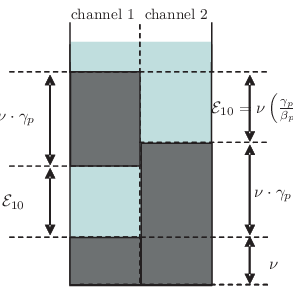
The described solution is similar, yet not identical with the water–filling solution and it can be interpreted as an intercepted water–filling, see Figure 4. Note that in the absence of the upper “stone” block in channel 1, this figure would have represented a conventional water–filling. The region pinched between stone blocks of channel 1 and 2 can be thought of a leakage canal of zero volume, such that while the lower basin of channel 1 is being filled only.
From the described interpretation of intercepted water–filling in case of channels, we can devise the general solution for power allocation when and the values of and are arbitrary. The intercepted water–filling produces the optimal solution. We omit the rigorous proof here and provide only the main arguments. First, note that is always a concave function of . When the function is non–differentiable at one point, but is still concave, as it can be represented as a minimum of two concave functions [6]. In that case the intercepted water–filling implements the steepest ascent algorithm, which leads to a globally optimal solution.
| Per–channel blocks for Intercepted Water–Filling |
| • If , then the channel contains only one block of height • If , then the channel contains two blocks. The lower block starts from the bottom and has a height . The upper block starts at a height of . The height of the upper block is . |
In order to implement the intercepted water–filing, we use the following rather visual explanation. Based on we have to determine the height of the “stone” blocks for each channel, as well as the position of the upper stone block. This is summarized in Table I. Note that the upper block appears only in the channels in which the primary signal is decodable. Having decided the block levels/positions in the channels, the energy allocation can be done by water–filling and considering that the water is leaking through the side walls of the upper blocks in the channels.
Rather than giving the precise algorithmic steps for intercepted water–filling, we illustrate it by the example on Fig. 5. The chosen parameters for the channels are ; ; . If the total energy is:
- •
: all the energy is allocated to channel 1.
- •
: then is allocated to channel 1 and is allocated to channel 3.
- •
: energy is allocated to channel 1 and is allocated to channel 3
- •
: energy is allocated to channel 1, energy is allocated to channel 3 and energy is allocated to channel 2.
- •
: channel 1 gets , channel 2 gets , channel 3 gets .
Note that the total height of the blocks in a channel is equal to . This implies that, when the amount of energy is sufficiently high, such that the water–filling goes above the uppermost block (in this example ), then the power allocation of the intercepted water–filling is identical with the allocation of the conventional water–filling.
V Numerical Results
In this section we will provide a numerical illustration of the OIC in order to show the introduced gain as compared to the case when the primary interference is treated only as a noise.
Let us first consider a scenario with with the following setup. The primary system has a range of meters and it adjusts its power so as to have a predefined SNR of for a receiver at a distance which has a Line–of–sight (LOS) link to the BS. Let us now consider a secondary receiver at a distance and let which also has a LOS to the BS. Then the primary SNR at the distance is equal to:
| (34) |
where is the propagation coefficient. Let us assume that the secondary TX adjusts the power within the allowed range, such that the secondary SNR at the secondary RX is . Fig. 6 depicts the normalized achievable rate as a function of the normalized distance . Two values of are used, and dB, respectively and is a measure of the power applied in the secondary system. For each , two rate curves are plotted, without Interference Cancellation (No IC) and with opportunistic Interference Cancellation (OIC). Clearly, OIC leads to higher rate when , but is identical to the case without interference cancellation for , as the primary signal cannot be decoded when the secondary RX is at distances . For the OIC curves, the rate points in the region are achieved by the described strategy of superposition coding. It is very interesting to notice that the two OIC curves are close to each other for around . This means that the increase of the power for 10 dB in the secondary system has produced a small rate increase. On the other hand, for the region , the rate gain out of the 10 dB improvement in the SNR is more pronounced. Recall from (18) and (III-A) that the rate of the secondary signal that is decoded after decoding of the primary signal is equal to and does not depend on . Thus, we can conclude that for around , this signal carries the dominant portion of the data in the secondary system. On the other hand, the first layer of the superposition coding (the one decoded before the primary signal) brings rate improvement for values of closer to the edges of the observed region.
Another perspective for the same scenario is given by Fig. 7. We assume that the secondary system aims to achieve a data rate equal to [bps]. Let and denote the required secondary SNR to achieve without and with OIC, respectively. The figure plots [dB] for and demonstrates the immense difference in the required powers. This illustrates the fact that, for the same required secondary rate, the interference towards the surrounding systems (both primary and secondary) is markedly decreased when OIC is used.
Figures 8 and 9 show the evaluation results for a system with channels. When OIC is used, the intercepted water–filling is applied. For the case without interference cancellation, the conventional water–filling is used. The abscissa depicts the scalar value of the total applied energy by the secondary system. For a given value of , the normalized achievable rate is the sum of the rates for all 10 channels (achieved with intercepted water–filling) and the value is obtained by averaging over iterations. In each iteration, the value for a given channel is generated as , where is exponentially distributed variable with average value 1. This helps us to interpret the energy in terms of SNR: The average secondary SNR per channel is . Also, in each iteration, the value is generated randomly from an exponential variable with mean value . The value is generated randomly from an exponential variable with mean value 20 dB and 23 dB, respectively, for each of the two OIC curves. We can see that the opportunistic rate adaptation with intercepted water–filling can lead to significant rate improvements. As expected, when the secondary has less opportunity to decode the primary signal, such that the improvement over the case without interference cancellation is decreased.
Fig. 9 reveals what is the difference in the energy allocation between the conventional water–filling and the intercepted water–filling. Let denote the energy allocation vector with intercepted water–filling, while E denotes the energy allocation vector for conventional water–filling in the case no IC is applied. Clearly, for given , the sum of the components of each vector is equal to . The relative difference is calculated as . When the average required minimal SNR , the energy allocation vectors obtained with the OIC are closer to the ones obtained without IC. This is because, for higher , there is less chance that a given channel will apply an intercepted water–filling. The relative difference decreases as the energy increases. As stated in the previous section, when the total energy is sufficiently high, then the intercepted water–filling and the conventional water–filling yield to identical energy allocation vectors, but still different rates.
VI Conclusion
We have investigated the problem of spectrally efficient operation in a cognitive radio system under interference from a primary system. A secondary (cognitive) receiver (RX) observes a multiple access channel of two users, one user being the desired secondary transmitter (TX) and the other the undesired primary TX. However, the primary system selects the transmission rate independently of the secondary system. If the link from the primary TX to the secondary RX is weak, then the secondary RX is not able to decode the primary signal. In order to make the best use of the power over the secondary link, the secondary system should apply Opportunistic Interference Cancellation (OIC). With OIC, the secondary system cancels the interference from the primary system whenever such opportunity is created by (a) selection of the data rate in the primary system and (b) the link quality between the primary TX and the secondary RX. We derive the achievable data rate in the secondary system, which is a function of the power applied by the secondary system. The parameters of this function are the power received from the primary and the rate applied in the primary system. We have also devised a method that does not use time–sharing in order to achieve all the achievable rate pairs in the multiple–access channel. This method has a practical significance for a cognitive radio system, since it enables rate adaptation without requiring the primary system to perform a particular action. The derived rate adaptation function is then applied in the scenario when the secondary system uses multiple channels interfered by the primary. In this case, based on the observed state in each of the available channels, the secondary system should allocate the transmission power in a way that maximizes the achieved sum–rate. Due to the features of the derived rate adaptation function, the conventional water–filling cannot be used. Therefore, we have introduced the method of intercepted water–filling. We have presented numerical results that illustrate the benefit of the devised methods of OIC and the intercepted water–filling.
As a future work, we will consider the strategies for power/rate adaptation when there are multiple concurrent cognitive radio systems. Regarding the devised method of rate adaptation, we are planning to quantify the improvement that it brings when we consider finite packet length and practical (suboptimal) modulation and coding methods.
References
- [1] S. Haykin, “Cognitive radio: Brain-empowered wireless communications,” IEEE Trans. Inf. Theory, vol. 23, no. 2, Feb. 2005.
- [2] N. Devroye, P.Mitran, and V. Tarokh, “Limits on communications in a Cognitive Radio Channel,” IEEE Commun. Mag., radio communications supplement.
- [3] ——, “Achievable rates in cognitive radio channels,” IEEE Trans. Inf. Theory, vol. IT-52, May 2006.
- [4] T. M. Cover and J. A. Thomas, Elements of Information Theory. John Wiley & Sons Inc., 1991.
- [5] K. Nishimori, E. Bottega, H. Yomo, P. Popovski, Y. Takatori, R. Prasad, and S. Kubota, “Spatial availability for cognitive radio system under directional interference,” in Proc. 9th International Symposium on Wireless Personal Multimedia Communications (WPMC’06), Sep. 2006.
- [6] R. T. Rockafellar, Convex Analysis. Princeton University Press, 1970.