Chromohydrodynamical instabilities induced by relativistic jets

We shall consider the fluctuations of density, energy density, pressure and plasma velocity, around their stationary and colorless state described by $\bar{n}$, $\bar{\epsilon}$, $\bar{p}$ and $\bar{u}^{\mu}$ respectively. In order to study such fluctuations we linearize the chromohydrodynamic equations (1, 2), assuming the fluctuations to be small. Notice that in the stationary state the color current defined in Eq.(6) vanishes, indeed

and we will assume that in the stationary state no field $F^{\mu\nu}$ is present in the system. We define the space dependent fluctuations of the various quantities around their colorless values as

All the fluctuations can contain both colorless and colored components, therefore they can be decomposed as

where $\delta n_{0}$ is the colorless fluctuation, and $\delta n_{a}$ the corresponding colored components.

The state described by $\bar{n}$, $\bar{\epsilon}$, $\bar{p}$ and $\bar{u}^{\mu}$ is assumed to be stationary, colorless, and homogeneous on the scale of variation of the fluctuations and therefore we have that

Moreover, since we will consider only small deviations from the stationary state, we will assume that the following conditions are obeyed

Actually, $\delta n$, $\delta\epsilon$, $\delta p$ and $\delta u^{\mu}$ should be diagonalized to be comparable to the $\bar{n}$, $\bar{\epsilon}$, $\bar{p}$ and $\bar{u}^{\mu}$.

We now aim to determining the set of equations that the fluctuations $\delta n$, $\delta\epsilon$, $\delta p$ and $\delta u^{\mu}$ obey. Employing the equations (9) and (10) we can derive the expression of the fluctuation of $n^{\mu}$ and of $T^{\mu\nu}$ around their colorless and homogeneous values:

Upon using these expressions in Eqs. (1, 2), we obtain that $\delta u^{\mu}$, $\delta p$, $\delta\epsilon$ and $\delta n$ must obey the following equations:

These equations do not form a closed set and one more relation has to be provided. In hydrodynamical treatments, one usually imposes an Equation of State (EoS) of the form

and in this way one obtains a closed set of equations. For the applications we have in mind, we will consider that the conformal limit is reached, and further the effects of the particle density can be ignored. Thus we will use an Equation of State given by

where $c_{s}$ is the speed of sound, and in the conformal limit $c_{s}=1/\sqrt{3}$. We will however leave $c_{s}$ as a parameter, and use its value only in the numerical analysis of the equations.

We will study separately colorless and colored fluctuations. In order to obtain the equation governing the colorless fluctuation we take the trace of the Eqs. (II.1) obtaining

Whereas multiplying the Eqs. (II.1) by $\tau^{a}$ and taking the trace we gather the equations for colored hydrodynamical fluctuations:

where we have used the notation $(D_{\mu}X)_{a}\equiv\partial_{\mu}X^{a}+gf^{abc}A_{\mu}^{b}X^{c}$.

The colorless fluctuations of plasma velocity, energy density, pressure and density obey the Eqs. (II.1) that in momentum space read

where $k^{\mu}\equiv(\omega,{\bf k})$. Since pressure and energy density are related by the EoS (18), their variations are not independent and upon differentiating Eq. (18) we obtain that

Substituting this expression in Eqs. (III.1) we find the following equation for the fluctuations of the pressure:

while the fluctuations of the other quantities can be expressed as

In the plasma rest frame, $\bar{u}^{\mu}=(1,0,0,0)$, Eq. (23) simplifies to

which gives the standard expression of the sound waves in a plasma, reflecting the fact that all colorless hydrodynamical fluctuations propagate at the speed of sound.

Regarding the colored components of the fluctuations, Eqs. (II.1), we linearize in the $A$ fields as well. The reason is that we will be interested in the computation of the polarization tensor and expanding at the first order in $A$ is sufficient. One then finds

and the fluctuation of the pressure and the fluctuations of the energy density can be related using the EoS (18), that leads to $\delta p_{a}=c_{s}^{2}\delta\epsilon_{a}$ Manuel:2006hg,foot1.

Equations (27) and (29) relate the fluctuations of the density and energy density with the fluctuations of the velocity

and combining these expression with Eq. (22) we find that Eq. (29) can be rewritten as

The inverse of the operator on the left hand side of this equation can be determined observing that

where

Then one can solve Eq. (32) and the fluctuation of the hydrodynamic velocity takes the form

The fluctuation of the current induced by the fluctuation of the density and of the hydrodynamic velocity can be derived from Eq.(6) and is given by

Such fluctuations are related in linear response theory to fluctuations of the gauge fields via

where $\Pi^{\mu\nu}_{ab}$ is the polarization tensor. Considering that the linearized strength tensor equals $F^{\mu\nu}_{a}(k)=-ik^{\mu}A^{\nu}_{a}(k)+ik^{\nu}A^{\mu}_{a}(k)$, and upon substituting the values of the fluctuations of density and energy density in Eq.(36) we obtain that

One can easily check that the polarization tensor (38) is symmetric and transverse ($k_{\mu}\Pi^{\mu\nu}(k)=0$).

In the plasma rest frame, $\bar{u}^{\mu}=(1,0,0,0)$, the polarization tensor simplifies considerably and its components are given by

where

is the plasma frequency.

At the linear order, the Fourier transformed chromodynamic field $A^{\mu}(k)$ satisfies the equation of motion

where we have dropped the color indices $a,b$.

In order to determine the dispersion law for the gauge fields we define the dielectric tensor $\varepsilon^{ij}(k)$ according to

that in the plasma rest frame is given by

The dispersion equation can now be determined by computing the determinant of the matrix

and solving the equation

where we assumed the Coulomb gauge, ${\bf k}\cdot{\bf A}(k)=0$, and $A^{0}=0$, meaning that ${\bf E}=i\omega{\bf A}$.

Taking the wave vector in a given direction, say ${\bf k}=(k,0,0)$, one finds the following solutions to the dispersion relation

which correspond to longitudinal and transverse modes, respectively. Notice also that both modes are not damped. The reason is that we have neglected the dissipative terms in the hydrodynamical equations, assuming that the colored plasma on the time scale of interest to the present analysis can be approximated as an ideal fluid. In order to consider the damping of color fluctuations in the hydrodynamical limit one should include transport coefficients, such as color conductivity or color diffusion.

Let us compare the dispersion laws of the longitudinal and transverse modes obtained above with the corresponding results in kinetic theory. Using the hard thermal loop (HTL) effective theory one can determine the polarization tensor for the gauge fields. The dispersion laws in the limit $k\ll\omega$ for the longitudinal and transverse modes are given by Lebellac

respectively. The chromohydrodynamical approach reproduces the short time physics of kinetic theory in the domain $k\ll\omega$. There is a numerical discrepancy in the $k^{2}$ terms when comparing the two set of dispersion laws. The origin of such a discrepancy is that in order to go from transport theory to a fluid approach, one has to impose a relation between the energy and the pressure of the system that allows to discard all the higher momenta moments that are contained in the particle distribution function. Such an approximation, typical of an hydrodynamical approach, does not affect in any profound manner the physics described in the domain of applicability of the formalism.

Here we consider the case corresponding to ${\bf k}\parallel{\bf v}$, and choose ${\bf k}=(0,0,k)$ and ${\bf v}=(0,0,v)$. This case can be easily analyzed because for this orientation of $\bf k$ and $\bf v$ the dielectric tensor (54) and the matrix $M^{ij}_{t}$ defined in Eq.(56) are diagonal and the corresponding dispersion equation factorizes. Moreover, since $\bf k$ is parallel to $\bf v$ it is possible to define transverse and longitudinal modes with respect to the orientation of these vectors. We find two stable transverse modes with dispersion law

Notice that this dispersion law is analogous to the dispersion law that we obtained in Eq.(47) that describes the propagation of the transverse mode in a a plasma without a jet. The only difference is that the plasma frequency $\omega_{\rm p}$ has been replaced with $\omega_{\rm t}$. Therefore the only effect on the transverse modes due to the presence of the jet is to change the plasma frequency of the mode.

Regarding the longitudinal modes, they are given by the solution of the following equation:

In terms of the dimensionless variables defined in Eq. (57), the equation for the longitudinal modes (59) can be written as

This equation has two trivial solutions $x=0$, and four solutions corresponding to the roots of a quartic equation. As already mentioned we find that at most one mode is unstable. In the present case one of the longitudinal modes is unstable for $c_{s}<v<1$. Since the cases where $v=c_{s}$ and $v\to 1$ will play a special role for these modes, let us first consider the solutions of Eq. (59) for these two values of the velocity.

In the limit $v\to 1$, Eq. (59) simplifies to

with solution, $\omega^{2}=0$ and

This solution is the same that we have obtained for a plasma without a jet in Eq.(46). Therefore in the limit $v\to 1$, the longitudinal mode is stable and we see that a jet of particles moving at the speed of light can only affect the transverse modes , but they do not affect at all the longitudinal modes. This is related to the dimensional contraction which occurs in the eikonal limit Jackiw:1991ck, when it can be shown that the strength field tensor caused by a massless particle that moves at the speed of light is on the plane transverse to its motion.

In the case $v=c_{s}$ it is possible to find one simple analytical solution (apart from the trivial solution $\omega^{2}=0$ and Eq. (58)) which is given by

whereas three more solutions correspond to the roots of

The discriminant of this equation is negative for $b<1$ meaning that the three solutions of this equation are always real and the corresponding modes stable.

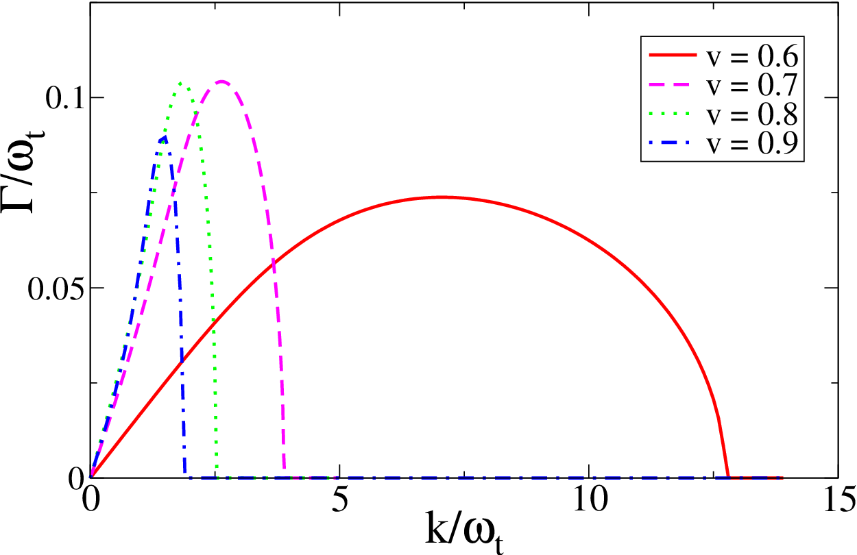
We now turn to a numerical study of the non-trivial solutions of Eq. (60) as a function of the parameters $b$ and $v$. We find a solution with a positive imaginary part for any non-vanishing value of $b$ and for $v$ larger than $c_{s}$. Such a solution corresponds to the unstable longitudinal collective mode of the system. In Fig. 1 we have reported the plot of the imaginary part of the frequency, $\Gamma$, of the this longitudinal mode as a function of $k/\omega_{t}$, for $b=0.02$ and for four different values of the velocity of the jet: $v=0.6$ full (red online) line; $v=0.7$, dashed (magenta online) line; $v=0.8$, full (green online) line; $v=0.9$, dot-dashed (blue online) line. For any value of the velocity smaller or equal the speed of sound we numerically find $\Gamma=0$. For values of $v$ larger than the speed of sound and less than $1$ this collective mode becomes unstable in a range of values of the momentum $k<k_{\rm max}$. For small values of $k$, $\Gamma$ increases with increasing momentum and reaches a peak. Then it decreases and at $k_{\rm max}$ becomes zero. As can be seen in Fig. 1 for $v>c_{s}$, the value of $k_{\rm max}$ decreases with increasing velocity.

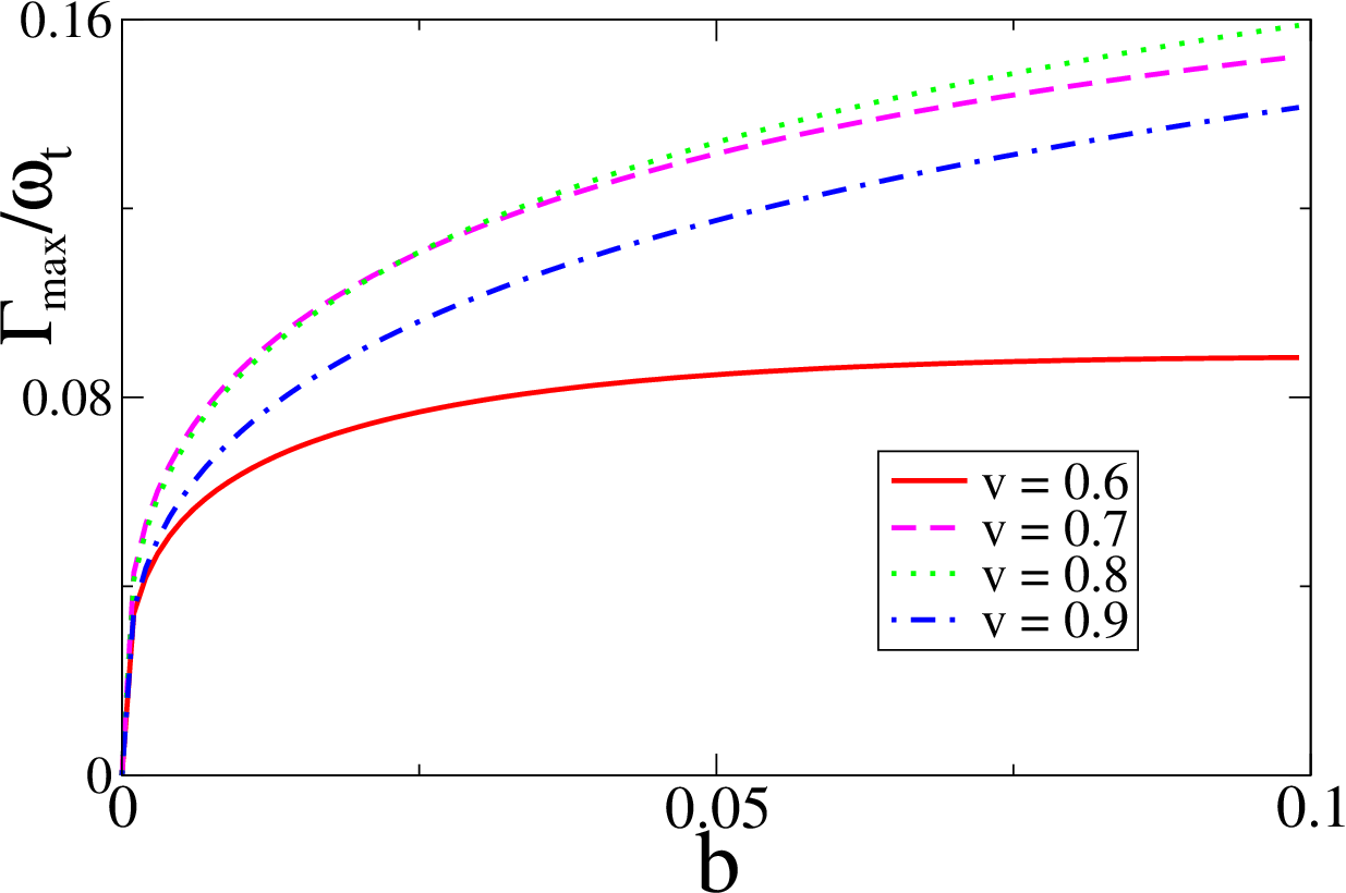
The value of $\Gamma$ at the peak, that we will indicate with $\Gamma_{\rm max}$, depends on $v$ and $b$. In Fig. 2 we present the plot of $\Gamma_{\rm max}$ as a function of $b$ for four values of the jet velocity: $v=0.6$ full (red online) line; $v=0.7$, dashed (magenta online) line; $v=0.8$, full (green online) line; $v=0.9$, dot-dashed (blue online) line. Note that independent of the value of $v$, for $b=0$, we obtain that $\Gamma=0$. In this case the plasma frequency of the jet is zero and corresponds to the case where the system consists of the plasma only. Indeed, for $b=0$, the dielectric tensor (54) does not have any contribution from the jet and therefore all the collective modes are stable, as shown in the previous Section. With increasing values of $b$, i.e. of the plasma frequency of the jet, $\Gamma_{\rm max}$ increases, meaning that to larger values of the density of the jet (for fixed values of $g$ and $\bar{\epsilon}_{\rm jet}+\bar{p}_{\rm jet}$) correspond larger instabilities. Moreover, for values of $b\lesssim 0.01$ the value of $\Gamma_{\rm max}$ increases quickly with increasing $b$ whereas for larger values of $b$, $\Gamma_{\rm max}$ becomes less sensitive to the actual value of $b$. In particular for $v=0.6$, $\Gamma_{\rm max}$ saturates at $\sim 0.09\,\omega_{\rm t}$. As a function of the velocity we find that for a given value of $b$ the value of $\Gamma_{\rm max}$ increases with increasing velocity for $c_{s}<v\lesssim 0.7$. For $v\sim 0.7-0.8$ the value of $\Gamma_{\rm max}$ reaches its maximum value and then for larger values of the velocity decreases and eventually in the ultrarelativistic case $v\to 1$ we find that the frequency of the longitudinal mode becomes real for all the values of $k$.

We now consider the case corresponding to ${\bf k}$ orthogonal to ${\bf v}$, choosing ${\bf k}=(k,0,0)$ and ${\bf v}=(0,0,v)$. In this case the matrix $M^{ij}_{t}$ defined in Eq.(56) is block diagonal. One block is one-dimensional and corresponds to the component $M^{yy}_{t}$. The other block is two-dimensional and corresponds to the components of $M^{ij}_{t}$ with indices $i,j=x,z$. Therefore the dispersion equation (56) factorizes into two equations. Regarding the one-dimensional block it describes a mode orthogonal to both $\bf k$ and $\bf v$. This mode is stable and has dispersion law

This dispersion law is analogous to the dispersion law for the transverse mode for a plasma without a jet, given in Eq.(47), with the plasma frequency $\omega_{\rm p}$ replaced with $\omega_{\rm t}$. The remaining collective modes are solutions of the equation

Using the variables defined in Eq. (57), one can rewrite this equation as

where we have already factored out the trivial solution $x^{2}=0$.

Also in this case we find that for $v\lesssim c_{s}$ no mode is unstable and for $v>c_{s}$ only one mode is unstable in a certain range of values of the momentum. We have numerically studied the solutions of Eq (67) and we have reported the results in Fig. 3 and Fig. 4. In Fig. 3 it is shown the plot of the imaginary part of $\omega$ for $b=0.02$, as a function of $k$ for five different values of the jet velocity: $v=0.6$, full (red online) line; $v=0.7$, dashed (magenta online) line; $v=0.8$, full (green online) line; $v=0.9$, dot-dashed (blue online) line; $v=1$ dot-dot-dashed (black) line.

The largest value of $k$ where the orthogonal mode is unstable is a monotonic increasing function of $v$ and it diverges for $v\to 1$. Also the value of the imaginary part of $\Gamma$ at the peak, $\Gamma_{\rm max}$, increase with increasing $v$, but for $v\to 1$ reaches a maximum finite value. The behavior of the largest value of the imaginary part of the frequency, $\Gamma_{\rm max}$, as a function of $b$, for various values of the velocity, is reported in Fig. 4. With increasing values of $b$, i.e. with increasing value of the plasma frequency of the jet, the value of $\Gamma_{\rm max}$ increases. Moreover, for a given value of $b$, the larger the velocity of the jet, the larger is the value of $\Gamma_{\rm max}$.

In the previous two Subsections we have analyzed the behavior of the unstable mode of the plasma for two values of the angle $\theta$ between $\bf k$ and $\bf v$. In particular in Section IV.1 we have considered $\theta=0$, corresponding to modes with $\bf k\parallel v$ and in Section IV.2 we have taken $\theta=\pi/2$, corresponding to modes with $\bf k\perp v$. A common feature of the two cases is that the value of $\Gamma_{\rm max}$ (corresponding to the largest value of the imaginary part of the frequency as a function of $|\bf k|$), increases with increasing values of the plasma frequency of the jet. Regarding the dependence of $\Gamma_{\rm max}$ on the value of the velocity of the jet $v$ one can see, comparing the plots in Fig.  4 with those in Fig.  2, that for ultrarelativistic jet the modes with $\bf k\perp v$ dominate the modes with $\bf k\parallel v$. On the other hand, for velocity larger than the speed of sound, but $v\lesssim 0.9$ the longitudinal modes are dominant.

In this Subsection we analyze the general case, of an arbitrary angle $\theta$ and we will determine at which angle corresponds the most unstable mode as a function of $v$ and $b$. For definitiveness we choose ${\bf v}=(0,0,v)$ and ${\bf k}=(0,k\sin\theta,k\cos\theta)$.

The analysis of the dispersion laws for the modes with $\bf k\parallel v$ and $\bf k\perp v$ was simplified by the fact that in both cases the matrix $M^{ij}_{t}$ defined in Eq. (56) becomes block-diagonal and the corresponding equation for the dispersion laws factorizes. However, for arbitrary angle $\theta$ the matrix $M^{ij}_{t}$ is not block-diagonal. Then we will rely on a numerical solution of Eq. (56). Employing the definitions in Eq.(57) we obtain (apart from the two trivial solutions corresponding to $\omega=0$), that the six dispersion laws can be obtained from the roots of the equation