arXiv:0705.0983
CALT-68-2644
ITFA-2007-15
Nonsupersymmetric Brane/Antibrane Configurations
in Type IIA and Theory
Joseph Marsano1, Kyriakos Papadodimas2 and Masaki Shigemori1
1 California Institute of Technology 452-48, Pasadena, CA 91125, USA
2 Institute for Theoretical Physics, University of Amsterdam
Valckenierstraat 65, 1018 XE Amsterdam, The Netherlands
marsano@theory.caltech.edu, kpapado@science.uva.nl,
shige@theory.caltech.edu
We study metastable nonsupersymmetric configurations in type IIA string theory, obtained by suspending D4-branes and -branes between holomorphically curved NS5’s, which are related to those of hep-th/0610249 by -duality. When the numbers of branes and antibranes are the same, we are able to obtain an exact theory lift which can be used to reliably describe the vacuum configuration as a curved NS5 with dissolved RR flux for and as a curved M5 for . When our weakly coupled description is reliable, it is related by -duality to the deformed IIB geometry with flux of hep-th/0610249 with moduli exactly minimizing the potential derived therein using special geometry. Moreover, we can use a direct analysis of the action to argue that this agreement must also hold for the more general brane/antibrane configurations of hep-th/0610249. On the other hand, when our strongly coupled description is reliable, the M5 wraps a nonholomorphic minimal area curve that can exhibit quite different properties, suggesting that the residual structure remaining after spontaneous breaking of supersymmetry at tree level can be further broken by the effects of string interactions. Finally, we discuss the boundary condition issues raised in hep-th/0608157 for nonsupersymmetric IIA configurations, their implications for our setup, and their realization on the type IIB side.
1 Introduction and Summary
Following the publication of [1], the past year has seen a great deal of interest in the study of metastable supersymmetry-breaking vacua in supersymmetric gauge theories [2, 3, 4, 5, 6, 7], and string theory [8, 9, 10, 11, 12, 13, 14, 15, 16, 17, 18, 19, 20, 21, 22, 23, 24, 25, 26, 27, 28, 29, 30, 31, 32]. Because such configurations do not correspond to true vacua, many of the difficulties associated with the construction of realistic models of supersymmetry-breaking can be avoided. As such, the ideas of [1] have already found wide phenomenological application [33, 34, 35, 36, 37, 38, 39, 40, 41].
One particularly interesting system, proposed in [16], realizes metastability by wrapping branes and antibranes on vanishing 2-cycles of a Calabi-Yau threefold. The geometry can be engineered so that these 2-cycles are homologous but, nevertheless, attain a finite size away from the singular points, providing a barrier to brane/antibrane annihilation. Unlike previous examples, this setup is inherently stringy in that the decay process cannot be described by a quantum field theory with a finite number of degrees of freedom11 1 If one attempts to decouple stringy modes to get a gauge theory description, one needs to take , which in turn means that one has to simultaneously scale the distance between branes and antibranes to infinity in order to render the open string tachyon massive. Conversely, keeping the branes and antibranes a finite distance apart, as was considered in [16], implies that must also be finite and, indeed, is sufficiently large that a field theory description is available only for the deep IR physics near either the brane or the antibrane stack..
A particularly nice feature of this system is that it appears to be under fairly good calculational control. When the numbers of branes and antibranes are large, the authors of [16] suggest that one can apply the large duality story of [42, 43, 44, 45, 46] even in this nonsupersymmetric setting. In other words, we can effectively replace the branes by a deformed geometry with fluxes. Moreover, it is argued that the supersymmetry on the deformed Calabi-Yau is actually spontaneously broken by the opposite-sign fluxes, implying that both the superpotential and Kähler potential continue to be determined by special geometry. This makes it possible to perform controlled computations and study, for instance, the stabilization of the compact complex structure moduli.
1.1 Brane/antibrane configurations in type IIA
It has been well known for many years that geometrically engineered systems of this sort are -dual to Hanany-Witten type NS5/D4 configurations in type IIA theory [47, 48, 49]. In this description, one studies the vacuum configuration by noting that the NS5/D4 system can also be described by a single M5-brane extended along a potentially complicated 6-dimensional hypersurface. If one tunes the parameters appropriately, the M5 worldvolume theory is reliably approximated by the Nambu-Goto action and hence the vacuum configuration corresponds to an M5 extended along a minimal area surface.
What can one hope to gain from such a description? In supersymmetric examples, BPS arguments indicate that the (holomorphic) physics should not depend on so one expects that the vacuum configuration at all values of the coupling is simply that obtained by applying -duality to the IIB picture. We can verify this directly from the theory point of view by noting that the minimal area M5 reduces, at small , to a curved NS5-brane with flux which is -dual to the IIB deformed geometry in the supersymmetric vacuum [50, 51]. This provides a nice alternative way of understanding the large duality story of type IIB but does not teach us anything fundamentally new about the physics.
In the nonsupersymmetric case at hand, though, we do not know a priori whether the vacuum configuration is protected as one moves to different parameter regimes or not. This has two important consequences. First, it means that we must take care to understand the specific choices of parameters for which a description based on minimal area M5’s is valid. Second, it indicates that the physics in one regime, say strong coupling, need not resemble that in another, say weak coupling, and hence there may be something new to be learned from a IIA/M description depending on precisely when we can perform reliable computations there.


In this paper, we thus endeavor to use techniques of -theory to study the nonsupersymmetric brane/antibrane configurations that are obtained by applying -duality to the system of [16], namely that with D5’s and ’s placed at conifold singularities in a local Calabi-Yau in type IIB22 2 Some comments on the IIA description have been made previously in [17].,33 3 Nonsupersymmetric brane configurations in IIA have been studied before, for example by the authors of [52, 53]. Unlike ours, the setups studied there are stable.. Specifically, the setup on which we focus most of our attention is that illustrated in figure 1(a) and consists of a pair of quadratically curved NS5-branes with stacks of D4’s and ’s suspended between them. From the point of view of theory, this system is described by a single M5-brane which, for parameter regimes in which the Nambu-Goto piece of the worldvolume theory is reliable, simply wraps a minimal area surface. There are two distinct parameter regimes for which this is the case and an analysis based on minimal area surfaces is justified. One lies at strong coupling, where the radius is large and the M5 curvature small in 11-dimensional Planck units. The other, which does not seem to receive as much attention in the literature44 4 The reason perhaps is that one typically is interested in the gauge theory limit where the scales of the system become substringy and the Nambu-Goto action ceases to be meaningful., lies at weak coupling. There, the M5 is more appropriately viewed as an NS5 with dissolved RR flux. The worldvolume action of the NS5 is simply the dimensional reduction of that of the M5 and the reduced Nambu-Goto term is reliable provided the NS5 is weakly curved and a few other conditions, about which we will have more to say in section 3.2.2 and Appendix A, are met. To summarize, once we find a minimal area M5 curve with the right properties, we can use it to reliably describe our system as a curved M5 at strong coupling or a curved NS5 with flux at weak coupling provided we make appropriate choices of parameters.
When the numbers of branes and antibranes are equal, we are able to find an exact solution to the minimal area equations which has a number of interesting properties. First and foremost, if we consider the regime in which the solution reliably describes our system at weak coupling as a curved NS5 with flux, it simplifies significantly to a configuration that is indeed -dual to a deformed Calabi-Yau geometry with flux in type IIB. Moreover, the moduli of the Calabi-Yau as determined by the minimal area condition in IIA exactly solve the equations of motion which follow from the IIB potential derived in [16] using large duality and special geometry. Consequently, we are able to understand large duality, even in this nonsupersymmetric context, from the IIA point of view as the replacement of the configuration of figure 1(a) by a curved NS5-brane with flux.
Furthermore, we can extend this agreement to more general situations by studying the NS5 worldvolume action directly. In the regime at weak coupling where our analysis is reliable, we are able to explicitly demonstrate for arbitrary numbers of branes and antibranes that solving the equations of motion of this system is mathematically equivalent to starting with the deformed Calabi-Yau of type IIB and minimizing the potential obtained from special geometry.
That we find such agreement between the IIB and IIA pictures is slightly nontrivial and, for reasons that we now explain, further supports the idea that these brane/antibrane setups exhibit a degree of protection, at least at small string coupling. In particular, our IIA analysis implicitly assumes that the circle on which we perform -duality is large in string units while reliability of the computations of [16] requires instead that the dual circle on the IIB side be large. Consequently, the two descriptions we are comparing correspond to quite different parameter regimes. For supersymmetric situations, one does not worry about this so much because the usual BPS arguments suggest that the system is protected as one varies this radius. When supersymmetry is broken, though, this is not expected to be the case unless there is some additional structure present. As alluded to before, the authors of [16] have argued that the brane/antibrane systems under consideration still maintain some residual structure from supersymmetry because, at least at string tree level, it is broken spontaneously via FI terms. It is this fact that must be responsible for our ability to successfully relate the IIB and IIA stories at weak coupling.
Given this success, it is natural to ask whether or not our system remains protected, in any sense, as we move to the strong coupling regime. From our exact solution for the lift of figure 1(a) with equal numbers of D4’s and ’s, though, it is easy to see that this does not seem to be the case in general. The reason for this is that our solution exhibits new nonholomorphic features which are small when the weak coupling interpretation is reliable but which can become large when the strong coupling interpretation is reliable. The most obvious of these can be understood by noting that it is favorable for the D4 and stacks to tilt slightly as depicted in figure 1(b). This is because the energy cost associated with increasing their length is balanced by the decrease in energy achieved when the branes and antibranes move closer together. Such tilting significantly impacts the entire geometry of the resulting M5 curve because the D4’s and ’s pull on and “dimple” the NS5’s in a nonholomorphic way [54]. In supersymmetric setups, the direction of this “dimpling” is transverse to the NS5’s and gets combined with the RR gauge potential, or coordinate in the -theory language, to form a holomorphic quantity. In the case at hand, though, the ‘‘dimpling’’ is no longer transverse to the NS5’s and consequently nonholomorphicity is introduced throughout the curve, even at infinity55 5 This is not the only nonholomorphic deformation of the geometry that arises but it is the simplest to see without discussing any details of the solution.,66 6 As we shall explicitly demonstrate, the tilting described here becomes parametrically small when the minimal area surface reliably describes the system as an NS5 in IIA. When the minimal area surface reliably describes the system as an M5 in -theory, this need not be the case as we can choose it to be small or large..
Having an exact solution to the minimal area equations in hand permits us to not only see this nonholomorphic features explicitly but also to demonstrate that they are controlled, at least when our description can be trusted, by two parameters involving and various characteristic length scales of the geometry. It is important to note that, unlike at weak coupling, we can take these parameters to be large at strong coupling while maintaining reliability of our description. Hence, these features are truly present in at least some part of the parameter space and are not simply an artifact of our formalism breaking down. However, the nice structure of our solution77 7 In particular, the solution factorizes into a holomorphic piece, roughly coming from the D4’s, and an antiholomorphic piece, roughly coming from the ’s, when both parameters are small. Because each piece is separately holomorphic with respect to a different complex structure, each is individually supersymmetric but with respect to different sets of supercharges. In the absence of further backreaction which breaks this factorization, the system thus seems to exhibit spontaneous breaking of supersymmetry. Of course, our solution is not reliable everywhere so strictly speaking we only know for sure that this nice structure is exhibited in the parameter regimes discussed in Appendix A. seems to suggest that one can go further and conjecture that the parameters we find are the only ones relevant for determining the “severity” of supersymmetry breaking, meaning that the system remains “protected” whenever both are small.
To summarize, we find that using the intuition of -theory to view the configuration of figure 1(a) as a single object, namely an NS5 with flux at weak coupling or an M5 at strong coupling, allows us to not only obtain an alternative understanding of the large duality of [16] but also to probe the brane/antibrane system at strong coupling. From this we learn that various features of this system seem to be protected as the radius of the -dual circle is varied but that this protection does not persist throughout the full parameter space. In particular, there exists a regime at strong coupling where our description is reliable and new nonholomorphic features become important. In retrospect, perhaps it is not surprising that stringy interactions can remove the residual structure of the supersymmetry that is spontaneously broken at tree level. It is gratifying to see this explicitly, though, and to learn something about the physics of metastable nonsupersymmetric configurations in string theory at strong coupling.
1.2 Metastability of our configurations
Finally, because this system admits IIA and IIB descriptions that we understand well, it provides a nice example in which to study the subtleties pointed out in [12] and how they arise in the geometric engineering context. A main point of emphasis in [12] is that nonsupersymmetric configurations engineered in type IIA from NS5’s and D4’s of the type we consider here have different boundary conditions, once quantum effects are taken into account, from the supersymmetric configurations into which they can decay. We can see this quite easily by studying the configuration of figure 1(a), taking the numbers of branes and antibranes to be equal for simplicity. In the nonsupersymmetric configuration, D4’s and ’s pull on the NS5’s and dimple them as mentioned above in a manner that extends out toward infinity. The supersymmetric configuration that remains after the branes annihilate, though, has no such bending because there are no longer any D4’s or ’s to cause it. From this, it is clear that the configurations have dramatically different boundary conditions at infinity and hence should be viewed as states in different quantum theories.
Does this mean that the nonsupersymmetric configurations we consider are quantum mechanically stable? It appears to us that the answer is no. By annihilating the fluxes on the curved NS5-brane, the system can indeed lower its energy and consequently it is favorable to do so via a tunneling process. Once the fluxes are gone, though, one can no longer support the nontrivial curvature of the NS5-brane and it begins to straighten. This is much like following the “quasikink” solution of [12] as the kink moves toward infinity88 8 More precisely, the “quasikink” of [12] was actually the opposite of what we discuss here with a supersymmetry-breaking configuration in the interior glued to supersymmetric boundary conditions. The idea is the same, however.. Because the kink never actually reaches infinity in finite time, the system exhibits a runaway behavior. The decay wants to end, but the final state at which it can end has moved off to infinity and hence left the theory entirely. This sort of picture has also been recently advocated in [23].
As a result, our configurations are not in the spirit of [1] in that they are not metastable supersymmetry breaking configurations in a supersymmetric theory. They are indeed metastable but, because of the boundary conditions, the theory in which they live is not supersymmetric. Instead, supersymmetry is broken by a runaway potential in a manner that seems to be qualitatively similar to [55].
What does all of this mean from the type IIB point of view? There, the bending of NS5’s corresponds to turning on nontrivial NS 2-form while energy stored in the NS5 tension is identified with the energy of NS 3-form flux . When the RR-fluxes and “anti”-RR-fluxes annihilate one another, the nontrivial can no longer be supported and relaxes just as the NS5’s did on the IIA side. The picture of the decay process we had before thus carries over entirely, complete with runaway behavior.
There is a distinct difference, however, between the philosophy behind typical NS5/D4 constructions in the literature and studies of the local Calabi-Yau configurations to which they are related by -duality which affects how one interprets these results. When one engineers gauge theories and other perhaps nonsupersymmetric setups using extended NS5’s and D4’s in type IIA, it is usually assumed from the outset that the full theory under consideration is truly 10-dimensional type IIA with fully noncompact branes. This means, for instance, that gauge theories realized in this manner are provided with a specific UV completion from the outset, namely MQCD99 9 In particular, this is precisely the situation studied by the authors of [12].. That is not to say that a local interpretation of these configurations is not possible but rather that it does not seem as natural in the IIA context.
On the other hand, the philosophy behind local type IIB constructions is quite different. One imagines that the local Calabi-Yau is capturing the physics in a particular region of a larger, compact Calabi-Yau. The situation is quite similar to effective field theory in that one imposes a cutoff scale in order to perform computations and specifies the values of noncompact moduli, which play the role of ‘‘coupling constants’’, at that scale. Of course, one can take the full noncompact Calabi-Yau seriously by taking the cutoff scale to infinity1010 10 One also tries to keep IR quantities fixed in this limit. Quantities for which this is possible are well-described by effective field theory.. This would correspond to UV-completing the effective local description into the -dual of MQCD. Typically, though, this is not our interest as compact situations are more realistic for practical applications.
Nevertheless, we learn something very important about these local IIB constructions from the subtleties that arose in type IIA. While we can study the tunneling process by which the fluxes and “anti”-fluxes annihilate in a local context, the eventual endpoint of the decay is highly dependent on how we UV-complete the local configuration into a compact Calabi-Yau. This is already evident from the computations in [16], where the energy difference between the supersymmetric and nonsupersymmetric configurations computed in a regularization scheme with finite cutoff exhibits an explicit dependence on that cutoff which cannot be removed. The lesson here seems to be that, while local constructions are useful for studying some aspects of metastable systems in string theory, one must be careful of the inherent limitations of such descriptions and take care to ask questions which they are well-suited to answer.
1.3 Outline of the paper
The organization of this paper is as follows. In section 2, we introduce the type IIB and IIA constructions that shall be the focal point of our work and review their relation to one another via -duality. In section 3, we review the relation between these approaches in two supersymmetric examples. In the first, we consider branes at a single conifold singularity in type IIB and their -dual description in terms of a pair of NS5’s with a single stack of D4’s suspended between them. This will allow us to review the basic philosophy behind the construction of parametric M5 curves. In the second example, we consider branes at a pair of conifold singularities and their -dual description in terms of quadratically bent NS5’s with two stacks of D4’s suspended between them. This will allow us to introduce a formalism for constructing genus-1 M5 curves parametrically which will be required when considering nonsupersymmetric configurations. In section 4, we turn to the brane/antibrane system of [16], its -dual description in type IIA, and the exact -theory lift. In section 5, we discuss various things we might learn from our solution regarding the “severity” of supersymmetry breaking, address issues related to boundary conditions and decays in greater detail, and finally mention a few possible future directions. The appendices include various technical details.
2 Preliminaries
In this section, we discuss the local Calabi-Yau geometries which play an essential role in the IIB constructions of interest [43, 44, 45] as well as the type IIA brane setups [54, 56] to which they are related by -duality [47, 48, 49]. Both of these are well-known, but we review them here for completeness and in order to make precise the specific -duality dictionary we shall be using.
2.1 IIB geometric constructions
We begin by considering the ALE space, which can be realized by the complex equation
| (2.1) |
One can view this as a fibration over the plane as in figure 2. The singularity at corresponds to a singular double-degeneration of the nontrivial in and can be removed by introducing a complex deformation as follows
| (2.2) |
The singular degeneration of at has now been replaced by smooth degenerations at . Fibering the over this interval yields an which has grown in place of the singularity as depicted in figure 2.


We can now construct a local Calabi-Yau threefold by fibering this deformed surface over a plane parametrized by a fourth complex parameter, , as in figure 3. This is easily accomplished in (2.2) by replacing the constant with a holomorphic function
| (2.3) |
For generic values of , the at the tip of the cone has finite volume but it degenerates at the zeros of . Moreover, because the roots of necessarily have multiplicity at least two, this degeneration is singular. To deal with this, one can proceed by analogy to what we did for itself, namely introduce a complex deformation that breaks the double-degeneracy
| (2.4) |


For generic nontrivial , each singular degeneration point of the will split into two points where the degeneration is smooth. Fibering the over an interval connecting these points then reveals that a compact has grown in place of the singularity. We will refer to these 3-cycles as the cycles of the geometry. The dual -cycles of the geometry are noncompact and can be obtained by fibering the over an interval beginning at one point of a given pair and extending to infinity along . An illustration of this can be found in figure 3.
Let us now consider “compactifying” type IIB on the undeformed local Calabi-Yau (2.3) and wrapping D5 branes on the degenerating . In order to prevent the effective 4d gauge coupling constant on the brane world-volume from diverging we must turn on a nontrivial NS-NS two-form field, , along the shrinking . A nontrivial -angle can be introduced by turning on the two-form as well. For a trivial fibration , the world-volume theory is simply SYM. A simple expansion of the DBI action reveals that the and fields determine the effective 4d complexified coupling via
| (2.5) |
where
| (2.6) |
Note that, as we shall continue to do throughout all that follows, we have set
| (2.7) |
The fields of this theory include an adjoint scalar which parametrizes the location of the branes along . Nontrivially fibering the deformed over the -plane restricts the branes to sit at the critical points of , where the ’s they wrap degenerate. From the gauge theory point of view, this nontrivial fibration corresponds to introducing a superpotential for the adjoint superfield1111 11 As the notation suggests, the function that appears in the local Calabi-Yau (2.3) is nothing more than the derivative of this superpotential [44]. [43, 44]. In what follows, we shall consider superpotentials that are polynomials of degree and restrict to deformations that are polynomials of degree 1212 12 In other words, we restrict to normalizable and log-normalizable complex structure deformations [43].. In these theories, the gauge group is Higgs’ed according to with denoting the number of branes sitting at the th critical point of .
While this geometric construction provides a nice visualization for the various Higgs branches that are present in the gauge theory, a direct analysis of the quantum dynamics is not immediately obvious because it requires going beyond the classical probe approximation for the D5-branes. It is by now well known that, in order to deal with this, one can use large duality [43] to replace D5’s at the singular points of the geometry (2.3) with RR 3-form flux wrapping ’s in the deformed geometry (2.4). In addition, we must also introduce some 3-form flux on the noncompact -cycles of (2.4) in accordance with the and that threaded the vanishing ’s of (2.3). The degrees of freedom of this system include chiral superfields associated to the sizes of the ’s and Abelian vector superfields obtained by reducing the 4-form potential. The former are identified with glueball superfields associated to the confined factors while the latter correspond to the “spectator” ’s.
Once we have replaced our brane configuration by deformed geometry with fluxes, the quantum dynamics becomes easy to study because it is captured by the well-known Gukov-Vafa-Witten (GVW) superpotential [57]
| (2.8) |
where is the holomorphic 3-form and is a combination of the NS-NS and RR 3-forms
| (2.9) |
Right away, however, we notice that noncompactness of the -cycles leads to problems because they have infinite holomorphic volume. In other words, the -periods of , which appear directly in (2.8), are divergent. In order to make (2.8) meaningful in practice, then, we must impose an arbitrary cutoff on integrals over the base. Concurrently, it is also necessary to specify the boundary conditions of the system at this cutoff scale. We can accomplish this by fixing the integrals of the 2-form potential over the fiber at
| (2.10) |
which is equivalent to specifying the regulated -flux along the noncompact -cycles. It is possible to incorporate -dependence in the boundary conditions in such a manner that explicit cutoff-dependence is removed from the superpotential (2.8). From the gauge theory point of view, this entire procedure is well-known. We have simply introduced a UV cutoff scale and specified the values of our “coupling constants” at that scale. Changes in cutoff scale must be accompanied by shifts in the couplings consistent with RG flow if we wish to preserve the IR physics.

Finally, we note that it is often useful in practice to integrate and over the fiber in order to reduce the problem to one involving 1-forms defined on a Riemann surface. We can do this explicitly for 1313 13 We insert the factor of for convenience in order to absorb the factor of 2 difference between the and cycles of the local Calabi-Yau, which pass along each cut once, and the and cycles of the reduced hyperelliptic curve, which encircle each cut, effectively passing along it twice (in equations, , ).
| (2.11) |
This 1-form is well-defined on the hyperelliptic curve
| (2.12) |
which can be visualized as a double-cover of the -plane with cuts connecting the various degeneration points. The and cycles of the local Calabi-Yau (3.1) now descend to and cycles on this curve1414 14 This is true up to the usual factors of 2, which we have absorbed into the definitions of and .. A convenient basis for these cycles is depicted in figure 4.
On the other hand, we do not have an explicit expression for or its corresponding reduced 1-form1515 15 The minus sign is inserted for convenience only.
| (2.13) |
but knowledge of the fluxes determines its periods along nontrivial cycles of (2.12) as follows1616 16 The factor of here is simply the fundamental unit of 3-form flux, , sourced by a single D5 brane.,1717 17 Note that we use upper indices for the fluxes as opposed to the lower indices denoting the number of branes. For branes, these are the same but for antibranes the sign is opposite.
| (2.14) | ||||
| (2.15) |
where we have defined
| (2.16) |
2.2 IIA brane constructions
Gauge theories that can be engineered using the type IIB constructions reviewed in the previous section can also be obtained from brane configurations in type IIA involving NS5’s and D4’s [54, 56, 58], as we now briefly review. In the following, we shall consider configurations with two NS5-branes and D4-branes extended along the 0123 directions. The NS5’s also extend along holomorphic curves of the form where
| (2.17) |
and are separated along by a distance . The D4’s are then suspended between the NS5’s along .

Let us begin by considering the case of parallel NS5-branes wrapping the curves in space. This is the situation depicted in figure 5. If we scale the length of the D4-branes along to zero, the theory on their worldvolume becomes effectively four-dimensional with gauge coupling constant given by
| (2.18) |
The brane configuration preserves 8 supercharges so this theory has supersymmetry in four dimensions. The vector superfield consists of an vector superfield as well as an adjoint chiral superfield which parametrizes the location of the D4’s along .
We can now introduce a superpotential for the adjoint superfield by extending the NS5-branes instead along the nontrivial curves [56, 59, 60, 58]
| (2.19) |
The various ways of distributing D4-branes at the critical points of correspond to the different Higgs branches of the theory.
While the classical brane picture is useful for visualizing the Higgs structure it is easy to see that, like the wrapped D5 brane configuration of the previous section, it obscures the quantum dynamics. The reason for this is that the setup does not describe a key element of the quantum system, namely backreaction of the D4’s on the NS5’s. In particular, it is well known that the NS5 throat is a region of large string coupling so it is difficult to analyze the NS5/D4 intersection, which plays a dominant role particularly when , in a IIA context.
To deal with this, Witten noted that NS5’s and D4’s are two different manifestations of the same object, namely the brane, and hence their intersection could be smoothed out by looking at this system from the point of view of -theory [54]. There, our NS5/D4 configuration is thought of instead as a single brane extended along a possibly complicated 6-dimensional hypersurface. At large and small 11-dimensional Planck length, , the worldvolume theory of the is effectively described by the Nambu-Goto action so its embedding into target space is one of minimal area. At small , on the other hand, this is better thought of as a curved NS5-brane with dissolved RR flux whose worldvolume theory is obtained by dimensional reduction. When the descendant of the Nambu-Goto term gives a reliable description of physics in the IR, this NS5 configuration can be obtained directly from the one at large by reducing along the -circle1818 18 For supersymmetric configurations, one typically performs this IIA reduction without a second thought as the M5 is protected in such cases from corrections that arise as is decreased. Because we are eventually interested in nonsupersymmetric configurations, we shall always be careful to specify when using the Nambu-Goto term at small is reliable.. In practice, this simply means that we reinterpret the coordinate in our M5 solutions as the appropriate RR gauge potential.
In the situation at hand, the brane extends along the 0123 directions and, due to supersymmetry, wraps a holomorphic curve in the remaining directions. Because each D4 stack in the IIA configuration fattens into a tube upon lifting to theory, the genus of is related to the number of such stacks by . It is convenient to use one of the complex coordinates, say , to parametrize this curve, permitting us to think of it as a double cover of the -plane with cuts1919 19 Of course, this relies on the fact that is actually hyperelliptic [54, 56]..
To determine the correct lift, we must impose the boundary conditions (2.19) along the and directions as well as require that the wrapping along be consistent with the D4 distribution in IIA. Turning first to , a hyperelliptic curve satisfying as can be written in the form
| (2.20) |
Note that this is precisely the curve on which the 1-form (2.11) was defined in the previous section. As such, we will continue to the basis of and cycles indicated in figure 4.
To deal with the constraint, we first combine with into a holomorphic variable [54]
| (2.21) |
where is the radius of the -circle. This is crucial because in the end we are looking for a holomorphic curve. With this definition, the condition that wrappings be consistent with the distribution of D4’s in the IIA reduction can be expressed as a constraint on the -periods of the 1-form
| (2.22) |
The -periods of , on the other hand, are related to the separation between the NS5’s along (and potentially along as well). Generically, will vary logarithmically with due to the fact that the D4’s pull on and “dimple” the NS5 [54]. As a result, integrals of along the noncompact -cycle will in general diverge, forcing us to introduce a cutoff on the -integration at an arbitrary point . This corresponds to introducing a UV cutoff in the gauge theory on the D4 worldvolume. We identify this separation with the (complexified) 4d gauge coupling at this scale
| (2.23) |
and hence the dependence on simply corresponds to RG flow. Once we have determined the holomorphic curve , we can reduce to IIA by simply reinterpreting , thus obtaining the curved NS5-brane with flux that results from backreaction of the D4’s.
The -theory description, as we have reviewed it so far, is purely on-shell so that, unlike the case of IIB with fluxes, we have no analog of the GVW superpotential that allows one to have an off-shell understanding of the system. Later, we will see one sense in which this description can be extended to capture some off-shell information. Another way this can be accomplished was suggested by Witten, who conjectured a form for the superpotential which captures off-shell physics of an wrapping [56]. In particular, if we let denote a reference surface homologous to and a 3-chain interpolating between the two, this superpotential he wrote is
| (2.24) |
Later, de Boer and de Haro [61] noted that this can be rewritten in the form
| (2.25) |
which is quite suggestive given the similarities between the 1-forms and here and the 1-forms (2.11) and (2.13) of the previous section. Of course, as we now review, this similarity is not an accident.
2.3 T-duality between IIA and IIB constructions
The above realizations of gauge theories in type IIA and IIB string theories are related by -duality [47, 48, 49, 50, 51]. Here we briefly review this relation and establish the mapping between quantities on both sides.
As we have seen, the type IIB construction is based on fibration of deformed ALE space (2.2) over the complex -plane. Consequently, if we understand the -duality between the ALE fiber over a point and the type IIA brane configuration at , the -duality relation between the whole systems will follow by applying it fiberwise. Therefore, we focus here on the -duality between ALE space and NS5-branes.
The deformed ALE space whose complex structure is displayed in (2.2) can be realized as a two-center Taub-NUT space (see e.g. [54], section 3).2020 20 Strictly speaking, a Taub-NUT space is ALF and we must take to make it ALE. The metric of the Euclidean -center Taub-NUT space is
| (2.26) |
Here , , is the position of the -th center in the base parametrized by , is a 1-form in , and is the metric for the remaining six directions 012345. If we -dualize the Taub-NUT metric (2.26) along using the standard Buscher rule [62], we obtain the IIA metric
| (2.27) |
Here is the -dual of whose periodicity is
| (2.28) |
and corresponds to in the last subsection. The metric (2.27) is nothing but the geometry produced by NS5-branes located at in flat space. In particular, if we set and (i.e., ), this shows that the deformed ALE space (2.2) is -dual to two NS5-branes at . Fibering this -duality over the -plane, we see that the local CY space (2.3) is -dual to two NS5-branes placed along the curve (2.19) in a flat space.
In the metric (2.27), though, the NS5-branes are delocalized (smeared) in the direction. However, in string theory, the NS5-branes are expected to become localized; indeed, it is known that the position of the IIA NS5-brane is dual to -field through certain 2-cycles in the IIB Taub-NUT geometry [63, 64]. Although one could study this localization of NS5-branes using worldsheet CFT techniques [65, 66], in Appendix B we have presented an alternative approach to determining the position of NS5-branes, which, to our knowledge, is new.
From (B.12), the 2-form fields in IIB are related to the distance between two NS5-branes in IIA in the following manner:
| (2.29) |
where was defined in (2.16) and in (2.21). The gauge theory couplings derived in IIB and IIA (Eqs. (2.5) and (2.18)) can be shown to be identical using this relation, as they should be. From (2.29) immediately follows also the correspondence between the following 1-forms in IIB and IIA:
| (2.30) |
From this relation, it is clear that the periods of in IIB, (2.14) and (2.15), are mapped into the periods of in IIA, (2.22) and (2.23). If we further note the equivalence between the following 1-forms in IIB and IIA (Eq. (2.11) and (2.20)):
| (2.31) |
we can see that the IIB superpotential (2.8) is equivalent to the IIA superpotential (2.25):
| (2.32) |
Summarizing the discussion so far, local CY geometries in type IIB are -dual to NS5-brane configurations in IIA, and the realization of gauge theories based on them are equivalent. There is one important issue that we have glossed over, though. The and circles are compact with radii and , respectively, and are related to each other by (2.28). In the IIB and IIA/M constructions in the previous sections, we treated these circles as if they were noncompact, by putting D5’s in a noncompact (local) CY in IIB and putting NS5’s and D4’s in noncompact in IIA (or an M5 in ). However, the validity of such “noncompact” description is not obvious, because if is large then is small, and vice versa. In the supersymmetric case, if we take the gauge theory limit (decoupling limit) where the scales of the system becomes substringy,2121 21 In the gauge theory limit in type IIA (IIB), we take the length of D4 (the size of the on which D5 is wrapping) and the distance between different D4 stacks (D5 stacks) to be substringy, such that and , where is the energy scale we are looking at. such a noncompact description can indeed be justified because the circle direction becomes much larger than the system size if we take . What if we do not take the gauge theory limit? Even then, as long as we focus on holomorphic quantities such as the curve (2.12), (2.20), we can still use the noncompact description. This is because these holomorphic quantities are protected by supersymmetry and do not depend on the scales of the system such as . Namely, we are free to take them to be infinite. In this sense, the noncompact IIB and IIA/M constructions in previous sections are -dual to each other if supersymmetry is preserved.
In the nonsupersymmetric case that we shall study later, things can be more subtle. In order for the fundamental string stretching between D-branes and anti-D-branes to be free of tachyonic modes, we must keep the distance between them to be at least of the order of the string length: . However, because of the relation (2.28), it is impossible to make both and much larger than at the same time. So, the full physics of the noncompact IIB and IIA/M constructions is not going to be the same. So, in a strict sense, by studying noncompact IIA/M system we will be exploring the nonsupersymmetric physics of a new system which is different from the IIB system studied in [16, 21].
However, even in the nonsupersymmetric case, it is possible that certain quantities are still protected, if the supersymmetry breaking is soft [67]. For such quantities, scale parameters are again irrelevant. Therefore, as far as such data are concerned, we can still say that the noncompact IIB and IIA/M constructions are in fact -dual to each other and describing the same physics. Indeed, we will see that certain quantities computed in IIA/M are the same as ones computed in IIB [16, 21], although supersymmetry is broken.
3 Two Supersymmetric Examples
We now proceed to elaborate upon the connection between the type IIB and IIA constructions reviewed in the previous section by looking at a pair of simple examples. Among other things, this will permit us to review the parametric representation of genus zero curves [56] and introduce the formalism for extending this sort of description to genus one situations in a more friendly, supersymmetric setting.
3.1 theory with quadratic superpotential — IIB
We begin with perhaps the simplest possible example, namely that of D5 branes at a conifold singularity [42, 43]. The relevant geometry is (2.3) with a quadratic superpotential of the form . After implementing large duality, we obtain the deformed geometry
| (3.1) |
with 3-form fluxes on the compact and noncompact cycles
| (3.2) |
This geometry has one modulus, , whose value is fixed dynamically. To study this further, we introduce and periods of the holomorphic form as usual
| (3.3) |
where is the prepotential. The field serves as an alternate means of parametrizing the (one-dimensional) moduli space of complex structures and, in fact, its relation to the modulus is easy to work out in this simple example
| (3.4) |
The expectation value of , and hence of , can now be obtained by minimizing the GVW superpotential (2.8). Using the Riemann bilinear relations, one can rewrite as
| (3.5) |
and immediately obtain the supersymmetric vacuum condition
| (3.6) |
where is the period ‘‘matrix’’ of the Calabi-Yau2222 22 We use a rather unconventional notation here, with denoting the period matrix as opposed to . The reason for this is to avoid confusion later when is used as the complex structure modulus of an auxiliary torus.:
| (3.7) |
Though the solution to (3.6) provides a perfectly good description of the complex structure of (3.1) at the supersymmetric vacuum, it is often desirable to translate this into a statement about the expectation value for . This requires us to compute , a task that is easily achieved in this simple example. Imposing a cutoff on -periods as discussed in the previous section, we find
| (3.8) |
where terms that vanish as have been dropped. Inverting this and applying (3.6) the expectation value immediately follows
| (3.9) |
In this expression, we have exhibited the explicit -dependence of the “coupling constant” that is needed to render cutoff-independent as well as introduced an “RG-invariant” scale 2323 23 The subscript refers to the fact that, in the theory we are studying, has degree . This is to distinguish from the analogous quantity introduced later for theories having of degree 2.
| (3.10) |
This completes our brief review of the system obtained by wrapping D5 branes at a conifold singularity. We have seen that the supersymmetric vacuum is described by the deformed geometry (3.1) with fluxes (3.2) and complex modulus (3.9).
3.2 theory with quadratic superpotential — IIA/M

We now proceed to study this system from the IIA/M perspective [56, 50, 51] . Applying -duality, we obtain a brane configuration with two NS5’s extended along the curves and separated along with D4’s suspended between. This configuration is depicted in figure 6. As discussed in section 2.2, in order to describe this system away from we should view it instead as an M5 extended along a genus zero holomorphic curve with boundary conditions
| (3.11) |
and embedding coordinate , defined in (2.21) to describe the wrapping along , satisfying
| (3.12) | ||||
| (3.13) |
Though an explicit representation of this curve is well-known [56], we shall review the parametric one here because it will more easily generalize to the nonsupersymmetric curves of interest later.
The curve we seek to study has genus zero so it can be parametrized by a single copy of the complex plane with a pair of marked points, corresponding to the preimages of on each of the two NS5-branes. For definiteness, we refer to the complex parameter as and place the marked points at and . At these points, the holomorphic functions and must diverge and, moreover, because the embedding is 1-1 near these divergences must come in the form of first order poles. Combined with the boundary conditions (3.11), this is sufficient to fix their form up to an overall rescaling
| (3.14) |
From this, it is easy to verify that and are related as in (2.20)
| (3.15) |
and hence that (3.14) provides a parametric description of the hyperelliptic curve depicted in figure 7(a). The and cycles shown there appear on the plane as illustrated in figure 7(b).

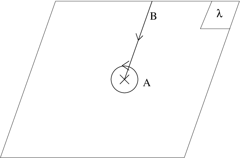
We now turn to the embedding coordinate , which characterizes wrapping along . A holomorphic with -period (3.12) is easily seen to be
| (3.16) |
The logarithmic behavior seen here, which we alluded to in the previous section, necessitates the introduction of a cutoff in order to study the -period constraint (3.13)
| (3.17) |
From this, we see that a holomorphic 1-form with the properties (3.12) and (3.13) exists on the hyperelliptic curve (3.14) provided the complex parameter satisfies
| (3.18) |
where is as in (3.10). This completely fixes the complex structure of the hyperelliptic curve (3.14)2424 24 Modulo choices parametrized by th roots of unity..
3.2.1 Comparison with IIB
If we interpret (3.14) and (3.16) as describing a curved NS5-brane with flux, the configuration at hand is -dual to a deformed geometry of the type (3.1) with flux (3.2). In fact, we can even verify that the modulus of our IIA configuration is identical to that determined in IIB by dynamics of the GVW superpotential (2.8). One way to do this, for instance, is to check the vacuum equation (3.6) directly. This can be done because the period “matrix” of the curve (3.14) is easy to compute in terms of
| (3.19) |
Using (3.18), it immediately follows that (3.6) is satisfied. Alternatively, we can make the comparison by computing directly. The -duality dictionary provides us with an expression for that is easy to evaluate on the IIA side
| (3.20) |
Using (3.18), we see that the expectation value (3.9) is reproduced. Consequently, we see that going from the NS5/D4 configuration of figure 6 to the curved NS5 with flux described by (3.14) and (3.16) is exactly -dual to the large duality in type IIB [50, 51]!
3.2.2 Reliability of the M5 and NS5 descriptions
Now that we have completed our description of the M5 configuration which reduces to that of figure 6 at , we must address the question of when this analysis is reliable. What we have found is a minimal area surface or, in other words, a solution to the equations of motion which follow from the Nambu-Goto contribution to the worldvolume action. Viewing our setup as a curved M5-brane, this is justified provided a number of conditions are met. First, we require that the curvature of the M5 be everywhere small in 11-dimensional Planck units and the radius of the circle large. Furthermore, we must avoid letting become too large in order to prevent the density of windings along from growing to the point that the M5 comes within a Planck length of intersecting itself. As discussed in Appendix A, one can demonstrate that all of these conditions are satisfied provided and the conditions (A.20) involving are satisfied.
On the other hand, we can attempt to provide a direct IIA interpretation of our setup as a curved NS5-brane with flux. Because the NS5 worldvolume action is simply the dimensional reduction of the M5 one [68], our analysis is valid in the IIA regime, where is identified with the appropriate RR gauge potential, provided we can restrict attention only to the descendant of the Nambu-Goto term. This, in turn, requires that the curvature of the NS5 be small in string units and that the flux not be too large2525 25 The reason for this is to prevent excited string states from becoming light. In particular, M2 branes ending on the M5 and wrapping in the -theory picture descend in IIA to strings with tension that can be made arbitrarily small unless is sufficiently small. See Appendix A.. We show in Appendix A that this leads to the constraints
| (3.21) |
where is as in (3.10) and is given by (3.20). Physically, these come about because when , for example, sets the scale of the “tubes” into which the D4’s blow up in the lift while determines the flux density. The symmetry under simply reflects our ability to interchange .
Outside of the regimes (A.20) and (3.21), our analysis based on the Nambu-Goto term of the worldvolume action is no longer reliable. One still expects the system to be described by an M5 along the curve described by (3.14) and (3.16) but this is dependent on a BPS argument that relies on supersymmetry.
3.3 theory with cubic superpotential — IIB
We now move on to the second example, namely that of D5 branes at the conifold singularities of the fibration (2.3) with
| (3.22) |
In particular, we have two singularities at at which we place and D5’s, respectively. After the geometric transition, we are left with the deformed geometry [43]
| (3.23) |
and 3-form fluxes
| (3.24) |
where .2626 26 We could actually choose and to differ by an integer. This corresponds to shifting the angle associated with one stack of branes by relative to the other stack. For simplicity, we take the angles identical so . This system has two complex moduli corresponding to the holomorphic volumes of the compact ’s
| (3.25) |
which can in turn be related to the complex deformation parameters and , though we do not do it explicitly here. Introducing the -period and period matrix as usual
| (3.26) |
we can write the GVW superpotential as
| (3.27) |
and obtain the supersymmetric vacuum condition
| (3.28) |
This specifies in terms of the fluxes and hence completely fixes the complex moduli. To translate this into a statement about the , it is necessary to determine the dependence of on the . This can be done using the results of [43], who compute the prepotential as an expansion in the variables
| (3.29) |
Applying their result, we find that is given by the following to leading order in the
| (3.30) |
This subsequently leads to the expectation values
| (3.31) |
where is the RG-invariant combination of and the cutoff
| (3.32) |
We see a posteriori that this result is valid in the regime and further corrections amount to an expansion in this parameter.
3.4 theory with cubic superpotential — IIA/M

We now turn to the description of this system in the IIA/M picture. The relevant brane configuration here consists of two NS5’s extended along the quadratic curves
| (3.33) |
and separated along with () D4-branes suspended in between at . This configuration is depicted in figure 8. The corresponding -theory lift is described by a genus one holomorphic curve with boundary conditions
| (3.34) |
and embedding coordinate satisfying2727 27 As in IIB (see footnote 26), we could choose to be different by an integer for and cycles. This would correspond to nontrivial wrapping of M5 along when one goes around the compact cycle .
| (3.35) | ||||
| (3.36) |
As in the genus zero case, an explicit representation is well-known but we shall seek a parametric description here. Such an approach may be unfamiliar, so we shall discuss it at length.
Because the desired curve has genus one, we shall parametrize it by a single complex variable subject to the identifications and where is the modulus of the torus. In all that follows, we will focus only on the fundamental parallelogram, which is depicted in figure 9(b). As in the genus zero case, we must specify two marked points and on the parallelogram as the preimages of the points at infinity on the NS5-branes. Unlike the previous example, though, the embedding is no longer one-to-one at infinity. This is due to the quadratic curving of the NS5’s and leads to the constraint that, while has single poles at and , necessarily has double poles at these points. The embedding coordinate , on the other hand, is multivalued on the -plane with a cut connecting and and monodromies consistent with (3.35) and (3.36).
With the analytic structure of , , and at hand we can in principle proceed to write them down. To do this in practice, though, we need the analog of the functions and which allowed us to introduce poles and cuts in the previous example. A convenient choice of building blocks for constructing genus one curves is based on the function2828 28 This collection of building blocks was recently used by [69] for essentially the same purpose as ours.
| (3.37) |
where
| (3.38) |
Because has a simple zero at , we see that near . This means that we can use to introduce branch points and derivatives of to introduce poles. In what follows, we shall adopt the notation
| (3.39) |
Detailed properties of these functions and their relation to Weierstrass elliptic functions can be found in Appendix C. The most important feature to keep in mind is that introduces an th order pole at the point . It is also worth noting here that the are elliptic for and have the following monodromies for
| (3.40) |
With our building blocks handy, we are now ready to begin writing general expressions for the embedding functions. We start with and , whose analytic structure was described above. If we add the requirement that near and , the most general possibility, up to constant shifts, is given by2929 29 The relative sign of and in is fixed by requiring to be elliptic while the relative sign of and in is obtained by requiring at and .
| (3.41) |
where we have inserted the constant shift so that behaves like (3.34) and is the separation between marked points
| (3.42) |
As described in Appendix C, it is possible to work out the polynomial relation between and explicitly. It takes the form of a hyperelliptic curve
| (3.43) |
with a particular quadratic polynomial in from which we can read off relations between the curve parameters and of (3.41) and the “physical” parameters and of (3.34)
| (3.44) |
The function appearing here is the Weierstrass -function.
We have thus seen that a holomorphic curve with the desired analytic properties along and corresponds to a hyperelliptic curve of the form (3.43) and admits the parametric representation (3.41). We have also found a convenient way to parametrize the moduli space of such curves, as they depend on two complex parameters, and . These are analogous to the quantities on the IIB side as they encode essentially the same information.
Let us finally turn our attention to the embedding coordinate , which is a multivalued function of satisfying (3.35) and (3.36). To determine its form, we must identify those cycles on the -plane that correspond to our and cycles. Illustrations of both representations of the hyperelliptic curve (3.43) which identify all the relevant cycles can be found in figure 9. Imposing the -periods (3.35) uniquely fixes the form of up to an integration constant, for which we make a convenient choice3030 30 Our choice of integration constant simplifies the limit used to obtain the local geometry near one of the D4 stacks. It also renders our curve invariant under a particular symmetry of the parametrization , , , .,3131 31 The relative coefficient of and is fixed by requiring to be elliptic.
| (3.45) |
where we defined
| (3.46) |


We can now fix the moduli and by imposing the -period constraints (3.36). First note that equivalence of the two noncompact -periods implies that
| (3.47) |
or in other words
| (3.48) |
This leads immediately to a relation between and
| (3.49) |
Evaluating the noncompact -periods then leads to the further condition
| (3.50) |
where
| (3.51) |
The conditions (3.49) and (3.50) are our final result for the constraints on moduli of the M5 curve.
3.4.1 Comparison with IIB
As in our genus zero example, there are several ways to compare with IIB. The most direct is to compute the period matrix of the elliptic curve (3.41) explicitly in terms of the parameters and . For this, we find
| (3.52) |
It is now easy to verify that the condition (3.28) on the moduli for supersymmetric vacua in IIB is solved exactly when (3.49) and (3.50) are satisfied.
If we are interested in computing the , though, these can also be determined by direct integration as discussed in Appendix C. In principle, they can be computed exactly as functions of and , though the expressions are somewhat complicated and hence not very enlightening. A natural limit to study is that of which, based on the identification of cycles in figure 9(b), we naively expect to be identified with a limit of large separation . Indeed, we can justify this expectation by noting that, in this regime, the ratio becomes
| (3.53) |
where we have suppressed terms that are further exponentially suppressed at large . Expanding the in this limit as well, we find
| (3.54) |
where the are as in (3.29). This agrees with the IIB result (3.31) that was obtained in the same regime. Because the moduli of the curve exactly solve the vacuum equation (3.28), this agreement will persist to all orders in the parameter . Though it was not our main objective, it is nice that the elliptic function formalism leads to exact results for the moduli as obtaining them from the IIB side requires a full solution of the Dijkgraaf-Vafa matrix model [70, 71, 72] (see also [69]).
3.4.2 Reliability of the M5 and NS5 descriptions
Finally, let us address the question of when our M5 and NS5 interpretations of the curve of (3.41) and (3.45) are reliable without the use of BPS arguments. For this, we can borrow many of the results of section 3.2.2 and Appendix A provided is sufficiently large. In this case, we note that the effective size of each tube is captured by the corresponding while the effective mass, obtained by expanding the superpotential (3.22) near one of its critical points, is given by . As usual, the conditions for a reliable M5 interpretation at strong coupling are straightforward but a bit complicated. These can be easily worked out from equation (A.20) in Appendix A.
The conditions for a reliable NS5 interpretation at weak coupling, on the other hand, take a fairly simple form
| (3.55) |
It is not difficult to see that these conditions can indeed be satisfied. Consider, for instance, the behavior of (3.55) at leading order in
| (3.56) |
These are easily seen to hold for a wide range of parameters. This condition will be of interest to us later when studying configurations with D4’s and ’s.
4 The Brane/Antibrane System
We now proceed with our study of IIA/M configurations obtained by applying -duality to the brane/antibrane system of [16]. After first reviewing the IIB construction of [16], we will discuss the NS5/D4 configuration and its theory lift.
4.1 Branes and antibranes on local CY in IIB
In the recent paper [16], it was suggested that interesting SUSY-breaking configurations could be constructed by wrapping D5’s and ’s at singular points of local Calabi-Yau. In particular, if the singular ’s wrapped by branes and antibranes are homologous, the absence of a conservation law preventing their eventual annihilation suggests that this system is metastable and will eventually decay.
Because supersymmetry is broken, it might seem that obtaining any quantitative information about the system is out of the question. However, it was suggested in [16] that the breaking is sufficiently soft that one retains a significant amount of computational control. In particular, they conjectured that large duality continues to hold, permitting one to replace the branes and antibranes with fluxes on a deformed geometry. Then, it was further argued that the SUSY of IIB strings on this deformed geometry is broken spontaneously by the fluxes, leading one to expect that essential aspects of the physics continue to be captured by the prepotential which, in turn, is determined by special geometry.
The simplest example of such a system has been considered at length in [16, 21] and consists of wrapping D5’s and ’s at the singular points of the fibration (2.3) with cubic superpotential (3.22). After the geometric transition, we are left with the deformed geometry (3.23), repeated here for convenience
| (4.1) |
and 3-form fluxes
| (4.2) |
We will use to refer to flux numbers, which can be negative, and to the number of branes or antibranes so that
| (4.3) |
We also take for simplicity as in the supersymmetric example of the previous section.
The presence of the fluxes (4.2) leads to generation of the superpotential
| (4.4) |
where as usual we define
| (4.5) |
The absence of solutions to the supersymmetric vacuum equation (3.28) 3232 32 That no solutions exist follows from the fact that is positive definite.
| (4.6) |
explicitly demonstrates that SUSY is broken and necessitates a computation of the scalar potential for the lowest components of to determine the actual vacuum. Because the breaking is spontaneous, it is natural to conjecture, as the authors of [16] did, that the Kähler potential of the system continues to be determined by special geometry
| (4.7) |
and hence that the scalar potential is given by
| (4.8) |
The moduli are now determined by minimizing this quantity. This was studied by the authors of [16] who found that, to leading order in the , the minimization equations can be written in the relatively simple form
| (4.9) |
and lead to the expectation values
| (4.10) |
where the are as in (3.29). In the above, we have implicitly defined the “RG-invariant” scale
| (4.11) |
As in the supersymmetric example of the previous section, we see that this approximation is valid for small . Subsequent corrections can in principle be determined using the Dijkgraaf-Vafa matrix model technology [70, 71, 72]. This was recently done in [21] and an interesting phase structure uncovered. We will see later how this structure arises in the IIA/M analysis.
4.2 Brane/antibrane configurations in type IIA and theory
We now consider the brane/antibrane configuration of [16] from the IIA/M point of view. Applying -duality, we find a pair of quadratically curved NS5-branes extended along the curves
| (4.12) |
and separated along . There are also D4’s suspended between the NS5’s at and ’s at . This configuration is depicted in figure 10.
This classical brane configuration fails to capture any quantum effects of the system and, strictly speaking, is valid only for . We expect that, just as in the supersymmetric examples discussed previously, quantum corrections will smooth out the NS5/D4 and NS5/ intersection points and also lead to a “dimpling” of the NS5’s. To study this process, we propose to follow the procedure adopted before and lift this configuration to theory. At large , this system is described by an brane wrapping a smooth minimal area surface in space. At small , this is more appropriately viewed as a curved NS5-brane with flux.
As usual, we shall work in a regime where the (NS5) worldvolume theory is reliably approximated by the Nambu-Goto action (or its descendant)
| (4.13) |
which, when reduced along the flat 0123 directions, looks similar to the “worldsheet” action of the bosonic string [56]. Standard analysis of this action indicates that a given surface is an extremum provided the embedding functions are harmonic on the “worldsheet”
| (4.14) |
and satisfy a ‘‘Virasoro’’-type constraint3333 33 We have assumed here a “target-space” metric of the form (4.15) where has been set to 1 as usual and the manifest -dependence has been introduced in accordance with the factor of in (2.21).
| (4.16) |
Notice that holomorphic embeddings automatically satisfy both conditions. In our situation, though, we do not expect to find a holomorphic curve because the presence of antibranes signals a breaking of supersymmetry.
Before proceeding let us note a few technical points. First, in order to prevent the open string tachyon from destabilizing our system, we need the separation between D4 and stacks to satisfy . Second, in what follows we will also take to be small when necessary, where is as in (4.11). Note that such a condition is not very stringent because, as we shall see later in section 4.5, if we make the physical assumption that then all solutions corresponding to true minima have this property.
4.2.1 First attempts at an -theory lift
For illustrative purposes, let us begin by attempting to construct a holomorphic lift of the configuration in figure 10 to see what goes wrong. The first step along this direction is to address the boundary conditions along and
| (4.17) |
We have already seen how to deal with these in the previous section. In particular, we saw that the resulting geometry must be a hyperelliptic curve which admits a parametric description of the form (3.41)
| (4.18) |
with and determined as in (3.44)
| (4.19) |
Our only task, then, is to write a holomorphic 1-form with the appropriate periods
| (4.20) |
The condition on the -periods uniquely fixes3434 34 As in the supersymmetric example of section 3.4, is fixed only up to an integration constant for which we make a particularly convenient choice.
| (4.21) |
If we now try to impose the -period constraints, though, we find a problem. In particular, because we must have
| (4.22) |
which in turn implies that
| (4.23) |
This is impossible because both and lie within the fundamental parallelogram by assumption. This result is not surprising. It simply illustrates that the obstruction to finding a holomorphic lift of the configuration in figure 10 is the lack of a well-defined embedding coordinate that yields the appropriate wrappings along .
This situation is easily improved, though, if we take away the constraint of holomorphy and instead simply require that be harmonic, continuing to satisfy one of the minimal area conditions (4.14). In this case, we can write it as the sum of a holomorphic and an antiholomorphic function and it is easy to find a two-parameter family of such with the right -periods3535 35 We have again made a convenient choice for the integration constant in .
| (4.24) |
We now have enough freedom to fix the -periods to whatever we like without saying anything about and . It is thus generically possible to write down a harmonic embedding with all the desired properties for arbitrary values of the moduli3636 36 More generally, a holomorphic 1-form on a genus curve of this type will have free parameters, which is enough freedom to fix the -periods but further imposing constraints on -periods fixes the moduli. On the other hand, a harmonic 1-form on a genus curve of this type will have free parameters, which is enough freedom to fix all periods for arbitrary values of the moduli..
It may seem that, with the moduli unfixed, we have too much freedom and indeed this is the case. With the introduction of nonholomorphic contributions to , we are now faced with the daunting task of addressing the nonlinear constraint (4.16), which is no longer satisfied. As we shall see, this will select a particular from the two-parameter family (4.24) and, in so doing, combine with the -period constraints to fix the moduli. For now, however, let us be very naive and try to use physical reasoning to pick a particular , postponing a further discussion of (4.16) to the next subsection.
At large separation , which we argued in the previous section corresponds to large , we expect the curve to roughly “factorize” into a holomorphic piece, describing the local geometry near the D4’s, and an antiholomorphic piece, describing the local geometry near the ’s. A realistic expectation, then, is that if we write as the sum of holomorphic and antiholomorphic parts
| (4.25) |
then the periods of will reflect only the contribution from the D4’s and the periods of only the contribution from the ’s when is large. Imposing this condition picks out the choice , in (4.24)
| (4.26) |
Further imposing the -period constraints for this particular then leads to the following conditions on and
| (4.27) |
Note the rough similarity of these equations to the vacuum equations (4.9) obtained on the IIB side at leading order in . We can make the comparison more explicit by using the expression (3.52) for the period matrix of the hyperelliptic curve (4.18) to write (4.9) as
| (4.28) |
It is now easy to see that (4.27) and (4.28) are equivalent and hence that the curve (4.18) with embedding coordinate (4.26) satisfying (3.35) and (3.36) has the same moduli as the nonsupersymmetric IIB vacuum at leading order in .
4.2.2 A few problems
Though our “physically”-motivated curve (4.18), (4.26) enjoys some success when comparing to IIB, two important problems remain. First, the connection with IIB is valid only at leading order in and fails to account for any further corrections. The second problem, which is not unrelated to the first, is that our curve fails to satisfy the additional constraint (4.16) and hence is not a true minimal area surface.
In fact, from (4.16) we see that the introduction of any nonholomorphic dependence to necessitates further nonholomorphic contributions to and . This further alters the geometry and, in particular, makes it impossible to write down an -theory lift of the configuration in figure 10 with a holomorphic relation between and . As a result, we cannot hope to obtain a geometry that is -dual to the local CY (4.1) with fluxes except in an approximate sense.
How then can we explain the nice agreement with IIB produced by our “physically”-motivated curve (4.18), (4.26)? Because it cannot be an exact solution, the best we can hope for is that, as alluded to above, it is an approximate one. To make this more precise, note that, at leading order in , the characteristic size of contributions to (4.16) from the embedding coordinate is while those from and are and , respectively3737 37 The easiest way to see this is by mapping the parameters , , and to the effective quantities and which determine the geometry near either brane stack. In particular, and . We now use the fact that the genus 0 curve has characteristic scales and to obtain the desired result. One can also obtain the scaling by studying the elliptic functions in (3.41) directly, but this is less transparent.. This means that the nonholomorphic contributions to typically scale like
| (4.29) |
and hence are suppressed relative to the holomorphic ones precisely when
| (4.30) |
Quite nicely, this is less stringent than the second of the conditions (3.56) required for our analysis based on the Nambu-Goto action to yield a reliable weakly-coupled IIA description of the configuration as a curved NS5-brane with flux3838 38 The second equation in (3.56) gives different conditions depending on the values of , but it is least stringent for , for which it is the same as (4.30).. In other words, when a IIA interpretation is reliable the nonholomorphic corrections to and are always suppressed!
This does not help at all with the problem of identifying the right from the 2-parameter family of possibilities (4.24), though. As we shall see, there are a couple of ways to deal with this. The most direct is to actually find an exact solution to (4.16) and study it in the limit of equation (4.30). This will be done in the next subsection. We could alternatively try to discern the behavior of the curve in this regime directly from the action without actually finding an exact solution. This will be addressed in section 4.4.
4.3 An exact -theory lift
Following the discussion above, we are led to conjecture that the configuration depicted in figure 10 can be lifted to an curve that, in the limit (4.30), is approximated by a holomorphic geometry of the form (4.18) with a suitable harmonic embedding coordinate . To test this conjecture, let us first search for an exact solution. This is most easily accomplished if the number of D4-branes, , is equal to the number of -branes,
| (4.31) |
because the additional symmetry leads to significant simplifications.
As described in Appendix D, the resulting curve satisfies
| (4.32) |
which causes a number of elliptic quantities to vanish and permits us to write a relatively-simple exact solution
| (4.33) |
where
| (4.34) |
and is one of the Weierstrass elliptic invariants as defined in Appendix C. This solution as written admits three free parameters, , , and . The first two are analogous to the quantities and in the supersymmetric curve (3.41) (3.45) and encode the boundary conditions of the curve along and . The third, , is determined in terms of the boundary data by the noncompact -period of .
There are a number of interesting features to this solution but let us focus for now on one in particular, namely that the functions , which exhibit logarithmic behavior and have described the bending of NS5’s along in our supersymmetric examples, make their appearance in 3939 39 Note that , , and their conjugates enter in a combination that is single-valued in a manner analogous to the function .. The reason for this is quite simple to understand. The branes and antibranes can lower their energy by moving closer together. Because of the NS5’s, though, this requires a rotation into the direction and carries an energy cost associated to the corresponding increase in length. In the equilibrium configuration, the D4’s and ’s are thus rotated a bit, changing the direction along which they pull on and “dimple” the NS5’s as illustrated in figure 11. This is directly reflected in the exact solution (4.33), where indicates the rotation angle.
4.3.1 The IIA regime
Let us now turn to the regime in which the configuration (4.33) can be reliably interpreted as a curved NS5-brane with flux. From the discussion of section 3.4.2, we see that this corresponds to the regime (3.56)
| (4.35) |
We now look for solutions with approximately holomorphic boundary conditions along and of the form
| (4.36) |
where ellipses are used to indicate the possibility of nonholomorphic terms which we have previously argued must be suppressed when the second condition of (4.35) is satisfied. To do this, let us rewrite (4.33) in the form of (4.18) with nonholomorphic corrections. Using (3.44) to relate curve parameters to the physical ones and , we obtain
| (4.37) |
From this, it is quite easy to see that the nonholomorphic contribution to is negligible provided4040 40 Note that we use the fact that , which is true when is small as we are assuming.
| (4.38) |
To determine precisely when the nonholomorphic contribution to is negligible, though, one must look a bit more closely at the properties of the elliptic functions . The largest contributions to the ratio come from the regions near near the D4 and “tubes” and hence near the midpoints between and . There, it is not difficult to show that the all scale like . This means that the first term of the expression for in (4.37) scales like 4141 41 Note in particular that the contribution from the is suppressed relative to that of the constant term . while the second term scales like . This means that the nonholomorphic contribution to is suppressed when
| (4.39) |
and hence that our solution reduces to a hyperelliptic curve along and with harmonic embedding coordinate when
| (4.40) |
Note that this condition is less stringent than what we expected from general reasoning (4.30). The reason for this is that while as a whole scales like , the division into holomorphic and antiholomorphic pieces is not symmetric. In particular, the holomorphic part of scales like but the antiholomorphic piece actually goes instead like . This means that can actually be a bit larger than our previous reasoning would have suggested. We expect this behavior to persist even for more general numbers of branes and antibranes so that nonholomorphic contributions to and can be neglected for a parameter range that is wider than what we need for the IIA interpretation to be reliable.
4.3.2 The Reduced Curve
Let us now focus on the regime (4.40) in which the nonholomorphic corrections to and in (4.37) can be dropped and we are left with the approximate solution
| (4.41) |
This geometry looks precisely like its supersymmetric counterpart (3.41) with the holomorphic embedding along (3.45) simply replaced by a harmonic one. Note that a very specific expression for has emerged with an extra factor of that we were unable to produce without the exact solution (4.33). As expected, this reduces to our guess (4.26) when is large because in this regime becomes
| (4.42) |
Without the solution (4.41) in hand, though, we were unable to say anything about possible subleading corrections away from the limit of infinite . Requiring the existence of an exact solution has now completely fixed the ambiguity of (4.24) for all values of .
This geometry is connected by -duality to a local CY of the form (4.1) with fluxes just as the large duality conjecture of [16] would suggest. But what about the moduli? We saw in the previous section that they agree in the limit but, armed with the correction terms in , can we go further?
Quite nicely, the answer to this question is a resounding yes. The complex structure of the curve (4.41) is completely fixed by the relations
| (4.43) |
| (4.44) |
where is as in (3.51) and the condition (4.44) arises from the -period constraint in (4.20).
As discussed in Appendix D, it is now easy to verify, using the expression (3.52) for the period matrix of the geometry (4.41), that and satisfying (4.43) exactly solve the equations of motion which follow from the IIB potential (4.8). In the regime where our exact solution (4.33) provides a reliable IIA description of the system in terms of a curved NS5-brane with flux, it is thus exactly -dual to the IIB system after the large transition to all orders in !
4.4 Direct analysis of the NS5 action
In order to better understand this agreement, we now turn to a direct study of the M5/NS5 action in the IIA regime (4.35) where the M5-brane can be described as an NS5-brane with flux.4242 42 The worldvolume action has previously been used to obtain Kähler potentials in [73]. We shall find that, in this limit, the IIB potential (4.8) makes a natural appearance and is responsible for fixing the moduli from the IIA/M point of view as well.
In M theory the M5-brane was curved in the directions. Upon reduction to IIA we expect a single NS5-brane curved in . The winding of the original M5-brane around the M-theory circle is encoded in the nontrivial configuration of the one-form field strength of the worldvolume theory of the NS5-brane in IIA. The relevant part of the NS5-brane Lagrangian is [68, 12]:
| (4.45) |
The NS5-brane configuration is specified by imposing the boundary conditions
| (4.46) |
at infinity, requiring the fluxes of to be consistent with the numbers of D4’s and ’s that we started with and fixing the logarithmic bending of at infinity.
Because the boundary conditions (4.46) along and are independent of and , the corresponding embedding functions can remain macroscopically large even regardless of the value of . This means that, provided we take to be sufficiently small, it is possible to obtain a parametric separation of scales relevant for the and parts of the geometry, respectively. Indeed, the second condition defining the IIA regime (4.35) is essentially just this because it is equivalent to imposing 4343 43 Recall that, on general grounds, we expect , , .. As a result, it is natural to separate the contribution to the induced metric coming from and write the NS5 worldvolume action as:
| (4.47) |
where the induced metric is that associated to the embedding coordinates and , treating as a constant. As explained above, the last two terms scale like . So defining:
| (4.48) |
and expanding to the first nontrivial order in we find
| (4.49) |
where is with respect to the metric .
Because we do not have to worry about the complications associated with finding exact solutions to the equations of motion, let us now be completely general here and try to minimize (4.49), starting with a configuration of NS5’s wrapping holomorphic curves
| (4.50) |
for a polynomial of degree and suspending arbitrary numbers of D4’s and ’s between the them at the critical points of . These configurations are related by -duality to the general ones of [16] with many conifold singularities. As we argued above we can replace the NS5’s and D4/ branes with a single NS5-brane with fluxes turned on. As usual, we shall denote the RR fluxes associated to these branes by with negative fluxes corresponding to antibranes. The embedding of the NS5-brane has to satisfy the boundary conditions:
| (4.51) |
at infinity and the periods of must be consistent with the fluxes as in (2.22) and (2.23)
| (4.52) |
If we consider only the first term of (4.49), ignoring the second for a moment, we find that the embedding described by and alone must be of minimal area. Since we impose holomorphic boundary conditions (4.51) at infinity, the entire surface must be holomorphic and we are again led to the family of hyperelliptic curves (2.12)
| (4.53) |
Note that the complex structure moduli of these curves are true flat directions of the first term in (4.49).
If we now consider only the second term in the action and minimize it with respect to for given and fixed embedding , the equations of motion imply that is a harmonic 1-form with respect to the induced metric . As we shall see explicitly in a moment, there is a unique harmonic 1-form with specified and periods for each value of the complex structure moduli of the curve (4.53).
This gives us our embedding but what about the moduli? Despite the fact that they correspond to flat directions of the first term in (4.49), this is not true of the second -dependent term. The moduli must therefore be chosen to minimize this quantity which, as we shall see, is nothing more than the IIB potential (4.8)4444 44 Consequently, we see that the two terms in (4.49) are, in a sense, not quite decoupled..
4.4.1 Construction of and the effective potential
To construct the harmonic form with the desired periods we proceed in the following way: we can parametrize the complex structure of the surface (4.53) by the periods of on the cycles:
| (4.54) |
The periods of on the cycles are determined by the holomorphic prepotential of the curve:
| (4.55) |
For each value of we want to construct a harmonic form on the surface with the desired periods. A harmonic form can be written as the sum of holomorphic and antiholomorphic forms. It is convenient to pick the following basis of holomorphic forms:
| (4.56) |
as they have nice periods on the A cycles:
| (4.57) |
and on the cycles:
| (4.58) |
where is the period matrix of the surface. The harmonic form is the sum of holomorphic and antiholomorphic forms:
| (4.59) |
The constraints (4.52) arising from imposing the specific and periods now determine the coefficients and completely in terms of and the period matrix in a manner that is straightforward to determine. Collecting into vectors and recalling that the are all identical, we can write the result in a compact form
| (4.60) |
To fix the moduli, we must now minimize (4.49). We focus on the second term because this is the only one that depends on the moduli. Using (4.60), we can write it directly in terms of and
| (4.61) |
This is precisely the effective potential on the IIB side obtained from special geometry [16] including the “zero-point shift” introduced therein. Consequently, we see that when we can reliably use the Nambu-Goto action to provide a reliable description of the system at weak coupling, the IIA picture quite generally reproduces the IIB story complete with some aspects of the off-shell physics. Note that from this point of view, the supersymmetric vacua also fall out nicely because any holomorphic that satisfies the constraints (4.52) automatically minimizes (4.49).
4.4.2 More on the connection with IIB
We can make the above agreement of the effective potentials computed in the IIB and IIA systems more transparent as follows. In IIB after the geometric transition we have a noncompact Calabi-Yau with fluxes. Without flux, the system would have flat directions parametrized by the complex structure moduli of the Calabi-Yau. The fluxes then create a potential for these moduli which stabilizes them. This potential (4.8) can be written suggestively as
| (4.62) |
where is the GVW superpotential (2.8) and the Kähler metric (4.7). Using standard results from rigid special geometry, it is not difficult to show that the scalar potential (4.62) is simply the “electromagnetic” energy of the flux of the system
| (4.63) |
Now the analogy with IIA should be clear. There, we started with two NS5-branes on the curves which get replaced by a single curved NS5 on a hyperelliptic curve of the form (2.12)
| (4.64) |
with 1-form flux on its worldvolume turned on and logarithmic bending along , both of which are combined into our complex coordinate . Without the flux and accompanying bending, the system has flat directions parametrized by the complex structure moduli of the hyperelliptic curve. The presence of nontrivial induces an effective potential for the moduli and lifts the degeneracy. The form of this potential is simply
| (4.65) |
which, given the identification (2.30)
| (4.66) |
is nicely consistent with -duality. Indeed, the tension of our bent NS5 with flux in IIA is directly identified with the energy stored in the nontrivial -flux in IIB.
4.5 When are our solutions true minima?
Before closing this section, let us come back to a subtle point that needs to be addressed. While we have demonstrated that our curves solve the equations of motion that follow from the IIB potential (4.8), we have not yet said anything about the nature of such solutions or even demonstrated that they exist in the first place. In particular, the moduli are fixed by (4.43) but inverting this equation to actually determine is nontrivial.
Precisely this issue was addressed on the IIB side in the recent paper [21], which used the Dijkgraaf-Vafa matrix model technology to compute subleading corrections to the potential (4.8) at large and study the structure of its critical points. They found a fairly intricate phase structure that should make an appearance in our formalism as well. In this section, we briefly comment further on this. While far from our original goal, one nice benefit of our work is that we have exact expressions in hand for both the solutions as well as the IIB potential for a cubic superpotential and equal numbers of branes and antibranes. This allows us to obtain exact results for many of the quantities which characterize the phase structure of [21]. It is important to point out, though, that the primary simplification arises not from a particular property of the IIA/M description itself but rather from the formalism we develop ed to study it4545 45 In particular, it is the parametrization of the complex moduli space by and that makes things simple. This does not come without a price, though, because the dictionary relating these quantities to the (C.39) is quite complicated., which does not easily generalize to curves with higher genus.
Before proceeding, let us first revisit the manner in which moduli are fixed from the IIA/M point of view. As described in detail in Appendix D, the conditions (4.43) follow directly from requiring that be periodic along the compact -cycle and imposing a symmetry on the full solution. The former is a necessary condition for existence of a well-defined curve4646 46 Of course, we could have taken to be periodic along the compact -cycle up to an integer multiple of , but we have chosen this integer to be zero for simplicity. while the latter is required because we imposed boundary conditions that preserve the obvious of the brane/antibrane system. Consequently, from the IIA/M point of view, simply having a smooth curve with the right boundary conditions already fixes all of the moduli except for the imaginary part of , which we hereafter refer to as
| (4.67) |
This quantity is finally fixed in terms of the boundary data by imposing the noncompact -period constraint in (4.20). The result is (4.44)
| (4.68) |
where we have implicitly used the fact that is real. As we saw in the previous section, imposing this condition is equivalent to further extremizing the approximate action (4.49) with respect to . The form of this action is equivalent to the IIB potential (4.8) and takes the form
| (4.69) |
In the IIA/M, approach, we are thus naturally led to study the potential (4.69) as a function of a single real parameter , which is easily seen to correspond essentially to the parameter in [21]. Critical points of this potential correspond to solutions of the full equations of motion. Because the expression (4.69) is exact for all , we should in principle be able to study the nature of its critical points in quantitative detail even away from the regime .
As a first use of (4.69), we can evaluate the potential at the degeneration point . In [21], it was argued that this quantity is independent of and indeed this can be verified explicitly
| (4.70) |
In fact, this is precisely the form of equation (103) of [21] with .
It is also fairly straightforward to study the qualitative structure of the critical points of (4.69), which correspond to solutions of (4.68). To do so, we note that
| (4.71) |
is a monotonically increasing function of satisfying4747 47 Because of these properties, we must have that in order prevent from diverging and becoming negative at small . The need for such a condition is clear as we do not expect to be able to take the cutoff smaller than the physical scale . The factor of can be understood by noting that the curve (3.41) becomes (4.72) at . The cuts extend from to 0 and are centered at . The above condition simply corresponds to the sensible requirement that the physical cutoff to be larger than this scale.
| (4.73) |
while is a monotonically decreasing function of satisfying
| (4.74) |
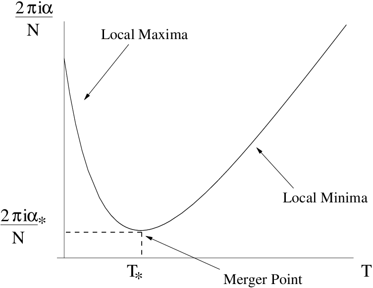
Consequently, if we fix and view (4.68) as defining a function as a function of , the situation is as depicted in figure 12 with attaining a minimum value at the point . What we see from this is that for there are two branches of solutions. At , these two branches merge so that for there are no solutions at all. From this structure, we can already conclude that one of the branches describes local minima and the other local maxima of (4.69). Physically, we expect that the branch yields the minima and indeed it is easy to see that this is the case by looking at the derivative of (4.69),
| (4.75) |
which of course vanishes when (4.68) is satisfied. Because is positive at both and it follows that, whenever has two critical points, the one at larger (smaller) is a local minimum (maximum), in agreement our expectations and the results of [21]. Also note that, depending on the size of , solutions along the branch may have higher or lower energy than the point (4.70) and hence do not always correspond to global minima of the potential. Sample plots of that exhibit all of these features are presented in figure 13.


What we have described above is precisely the phase structure of [21], to which we refer the reader for a more thorough discussion. The critical point corresponding to a particular choice of is determined by the equations
| (4.76) | ||||
| (4.77) |
Unfortunately, these expressions are quite complicated so, even though we can in principle solve for and in full generality, it is difficult to do so in practice without resorting to numerics. As noted in [21], though, one should be able to move all of the interesting physics to the regime of large , where (4.76) and (4.77) become more manageable, by tuning appropriately. To see this from (4.76) and (4.77), note that the LHS’s of both equations are monotonically increasing functions of and hence that and both grow as is increased. This means that we can always ensure that by choosing to be sufficiently large. Expanding (4.76) in this regime, we find
| (4.78) |
which, using (C.40), is equivalent at large to the condition for minimizing equation (87) of [21]. From this, we conclude that for
| (4.79) |
Turning now to equation (4.77), we can expand at large
| (4.80) |
and subsequently apply (4.79) to obtain equation (90) of [21]
| (4.81) |
Another regime in which (4.76) and (4.77) simplify is that of small but physically this is not very interesting because the description that we have in hand breaks down there. As discussed in [21], additional degrees of freedom that have not been accounted for enter the story. On the IIB side, D3 and D5 branes wrapping the shrinking compact cycle become important. On the IIA side, these correspond to D4 and D6 branes with boundaries on the curved NS5 which wrap the compact -cycle.
Of course, there is much more to say about the phase structure of this system than what we have described here. For this, we refer the reader to the discussion of [21], which can easily be translated to the IIA/M picture via -duality.
5 Discussion
In this section, we comment on various lessons that can be drawn from our IIA/M analysis. First, in section 5.1 we shall address the possible conclusions one can reach about the nature of supersymmetry breaking in these setups with particular attention paid to when some residual supersymmetric structure remains. Following this, we turn in section 5.2 to the implications that observations made in [12] have on our configurations, how they arise in the -dual type IIB setup, and the general lessons one can draw from them for studies of metastable nonsupersymmetric configurations in local contexts. Finally, in section 5.3 we address some open questions that would be interesting to study further.
5.1 Brane/antibrane configurations and spontaneous supersymmetry breaking
Though we have described our type IIA brane/antibrane configurations as being -dual to the IIB setups studied in [16], there is an important point that must be emphasized. All of our analysis has relied on the fact that the circle on which we perform -duality is large in the IIA picture. On the other hand, the analysis of [16] implicitly assumes that this circle is large on the IIB side so, in reality, the two approaches are focusing on quite different regions of parameter space. In supersymmetric situations, this typically is not important because BPS arguments guarantee that quantities such as the compact complex structure moduli in IIB are protected as the radius is varied. In our case, though, supersymmetry is broken so our ability to connect the IIB and IIA pictures at weak coupling indicates that some additional structure must be present there.
Indeed, the analysis of [16] relies quite heavily on the argument presented therein that, after the geometric transition, supersymmetry is spontaneously broken in these setups, at least at string tree level. This additional structure is what ensures that the Kähler potential determined from special geometry is reliable and can be used to compute the potential (4.8) that fixes the moduli. It must also be responsible for our successful comparison of the IIB and IIA pictures.
In a sense, then, our ability to reproduce the results of [16] in weakly coupled IIA despite the fact that we have essentially tuned the IIB radius to zero provides further evidence in support of the assertion made there that the breaking of supersymmetry is spontaneous, at least for some range of parameters. Moreover, we may be gaining a hint as to what parameters actually control the “severity” of supersymmetry breaking because the novel features of our solutions are controlled by the objects and . Whenever both of these quantities are small, the minimal area curve takes the form (4.41) and can be successfully compared to type IIB. On the other hand, when either is large, new phenomena such as the introduction of nonholomorphic bending along are introduced4848 48 Note that we can reliably turn on and/or while continuing to use our minimal area curve for a range of parameters at strong coupling so they are indeed real and can be studied reliably in the -theory regime.
Indeed, the very structure of our curve suggests that supersymmetry is spontaneously broken when and are small because there it factorizes into two pieces which are separately holomorphic but with respect to different complex structures. In other words, the solution factorizes in this regime into two pieces which are individually supersymmetric but preserve different sets of supercharges. It is only the simultaneous presence of both which leads to breaking of supersymmetry. This nice structure strongly suggests to us that supersymmetry thus remains spontaneously broken, and hence our solution remains reliable, even outside of the regimes discussed in Appendix A provided and are both small.
A natural question to ask now is whether or not the relevance of and can be understood more directly. At strong coupling, their importance is rather obvious because, as we have seen, they control the “backreaction” of the nonsupersymmetric fluxes, reflected by the nonholomorphicity of , on the geometry. When they become important, nonholomorphicity enters into and and destroys the nice factorized form alluded to above. Of course, we could have said essentially the same thing about our curved NS5 brane with flux at weak coupling.
A more difficult question, though, is how these parameters appear in the open string picture with the D4 and branes. There, it is well-known that the presence of the ’s leads, at string tree level, to the introduction of an FI -term which spontaneously breaks supersymmetry4949 49 for a review of this, see for instance [74].. Because there is no structure to prevent it, we expect that the breaking becomes more severe when string interactions are taken into account. One might therefore expect that the breaking remains spontaneous provided . From our exact solution, though, we see that it is also necessary for to be bounded in some sense. What, though, is the physical relevance of ?
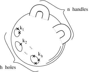
For this, consider an open string amplitude, given by inserting open string vertex operators, corresponding to fields living on D-branes, on a worldsheet . Let the worldsheet be a sphere with holes and handles added. There are boundaries on the worldsheet. Insert open string vertex operators on the -th boundary, where . Let the total number of vertex operators be . The amplitude then goes like
| (5.1) |
Here is the normalization constant for open string vertex operators and is the amplitude without insertions5050 50 Recall that , and adding a hole to a worldsheet gives a factor of while adding a handle gives a factor of ; this is how we got the above power of . . This leads to the term in the five-dimensional action on the D4/-branes:
| (5.2) |
where we denoted the fields collectively by . can be the adjoint or bifundamentals.
To get the conventional normalization where the kinetic terms have in front of them, let us rescale fields as . Then we have
| (5.3) |
If we integrate over , this becomes
| (5.4) |
where we defined a four-dimensional ’t Hooft coupling constant by
| (5.5) |
From (5.4), it is clear that counts the number of handles and counts the number of boundaries. Thus, we see that even if is small we can still get sizeable stringy corrections from provided is large enough.5151 51 It was noted in [75] that, in the limit with fixed , the gauge theories geometrically engineered by D-branes on CY singularities receive contributions only from disks and thus have only single-trace operators. Here we are refining and generalizing his argument by introducing parameters , , and . Determining precisely how large must be, though, is a more difficult question which requires a knowledge of how and appear in the various interaction terms (5.4). It would be very interesting to pursue this further and understand the relevance of the specific quantities and from this open string point of view.
5.2 Metastability and boundary conditions
We have constructed nonsupersymmetric configurations in type IIA/M theory by suspending D4’s and ’s between curved NS5’s. Because of their tension, D4’s and ’s pull and bend the NS5’s logarithmically in a manner that extends to infinity (Fig. 15(a)).
D4’s and ’s being separated by a potential barrier, this configuration is classically stable, but in quantum theory they can pair annihilate by quantum tunneling, as we have already discussed in the introduction.5252 52 For simplicity of the argument, we are assuming that the numbers of D4’s and ’s are the same, .,5353 53 A similar analysis of different configurations appeared in [23]. The time it takes for this tunneling process to occur can be estimated by a standard analysis, considering an instanton interpolating the initial and final configurations [16]. Note that, for the physics of this tunneling, the fact that the NS5’s are bent logarithmically does not matter; the D4 and know only about their vicinity and what is happening far away is irrelevant for this instantaneous process. This is very much as the -decay of a nucleus in an electric field; the decay rate, governed by quantum tunneling, is not affected by the electric field outside the nucleus. Once all the D4’s and ’s have pair annihilated (Fig. 15(b)), the tension that was holding NS5’s is no more and the NS5’s start to straighten (Fig. 15(c)). This part of the decay process proceeds according to the classical equation of motion, much as the fact that, once the -decay has taken place, the motion of the emitted positron in the electric field can be treated classically. The straightening of the NS5’s propagates outward (Fig. 15(c),(d)), but the time it takes for the straightening to reach the cutoff goes to infinity as one takes . Namely, in the limit, the system has a runaway instability. Note that, the energy released in this process becomes infinite as , because not only the mass of the D4/ but also the tension of the infinitely long bent NS5 gets converted into energy. Although here we explained the decay process in the IIA language for the sake of argument, but the decay process in M-theory is exactly the same.

This is in contrast with what happens if there is no logarithmic bending of NS5’s, which is the case if is strictly zero: . In that case, there is no “straightening” part of the above decay process, since the NS5’s are straight from the beginning (in the direction; in the directions they are holomorphically curved). So, the decay process ends in a finite time when the D4’s and ’s have gone through quantum tunneling and pair annihilated. The final configuration is a supersymmetric configuration of two NS5’s along the holomorphic curves,
| (5.6) |
However, for , which is the case we have been focusing on, there is logarithmic bending. Therefore, for , our nonsupersymmetric D4/ system and the supersymmetric system (5.6) have different boundary conditions for NS5’s at infinity. In general, to properly define the quantum theory of non-compact systems, one must specify the boundary conditions at infinity. This means that, the metastable configuration of Fig. 15(a) and the supersymmetric configuration (5.6) are not different states in the same theory but rather different states in different theories. Therefore, the former can never decay into the latter, which was the emphasis of [12].
Note that this does not mean that the configuration of Fig. 15(a) is stable. As we have seen, it does decay and shows a runaway instability. This is not at all in contradiction with [12] but actually [12] gives a nice interpretation of this runaway instability as follows: although our nonsupersymmetric system wants to decay into the supersymmetric configuration (5.6), it can only keep decaying forever toward the latter, because the latter does not lie in the same theory. The fact that the energy released in the process is infinite also implies that this process cannot end in a finite time.
In the above, we used the fact that the D4/ pull and bend the NS5’s to explain that the boundary conditions are different for nonsupersymmetric and supersymmetric configurations. An alternative way to understand this is the following. A D4-brane ending on an NS5 is a vortex charge for the 1-form field strength on the NS5 worldvolume theory. Because D4 and have opposite vortex charges, the total charge on each NS5 is . This is the same as for the supersymmetric configuration (5.6), which has no D4/ and hence no vortex charge. However, D4-branes ending on an NS5-brane act also as charges for the scalar field, with respect to which D4 and have the same charge. Therefore, the total charge is and is different from that of the supersymmetric configuration, which is zero. So, the two configurations have different charges and one cannot decay into the other.
The boundary condition being different for nonsupersymmetric and supersymmetric configurations can be understood in IIB also. If we wrap D5’s on 2-cycles in CY and turn on -field through them, D3 charges are also induced. A careful study of the system of field strengths shows that in the presence of these sources, the field has to grow logarithmically with , once we include the leading-order backreaction of the D5’s on the geometry5454 54 The easiest way to see the logarithmic running of is from the picture after the geometric transition. The running of is supposed to capture the RG flow running of the gauge coupling.. So, while at tree level we can specify the flux through the 2-cycles to be equal to a constant (which is the -dual statement of specifying the position of the NS5-brane to be constant), once we add D5’s and consider their backreaction, we see that grows logarithmically at infinity, necessarily modifying the boundary conditions of the system. Now the difference of boundary conditions is easy to see: if we start with D5’s and ’s, the logarithmic divergence of at infinity will be proportional to . On the other hand in the supersymmetric configuration, is constant and there is no logarithmic running. So the boundary conditions at infinity are different. Also the energy difference between the two configurations diverges logarithmically if we integrate the energy of the field over the entire space.
Finally, as we saw in section 4, the boundary condition difference in M theory is more serious. Besides the different logarithmic bending of the coordinate, we also have to change the asymptotic behavior on the plane to solve the minimal area equations.
5.3 Future directions
In the present paper, we studied nonsupersymmetric metastable configurations and found that they can be analyzed in a reliable way using the NS5/M5 worldvolume actions in various regimes of type IIA/M-theory.
We focused on the case of two D4/ stacks between two quadratically bent NS5-branes in type IIA, or, in the -dual IIB description, local CY geometry obtained by fibration. However, the method of nonholomorphic M5/NS5 curves is applicable to more complicated configurations. For example, flavors can be incorporated by including semi-infinite D4/-branes attached to NS5’s or by including D6-branes [54]. In particular, such systems should give us an -theory viewpoint to look at the nonsupersymmetric metastable states in gauge theory which were found in [1] and whose possible string theory embeddings were pursued in [10, 12]. It is also straightforward to generalize our method to -- quiver gauge theories obtained by stretching D4/-branes between multiple NS5’s, which is -dual [50, 51] to the local CY geometries obtained by -- fibrations [44, 45]. What is particularly interesting about such more general systems is that, nonsupersymmetric brane/antibrane configurations can be stable rather than metastable [53]. In such cases it may be possible to take the gauge theory limit and one may be able to study the “protection” of holomorphic quantities in gauge theory techniques.
Obtaining exact M5/NS5 curves in such more complicated systems will be increasingly difficult in practice, if not possible. However, the fact that for small the curve decomposes into the holomorphic part () and the harmonic part () must still hold, and we furthermore expect that the curve is protected in the same parameter regime because we conjecture that supersymmetry softly broken there. This may provide a tractable window in which one can study the vast nonsupersymmetric landscape of string/M-theory in a controlled way. Needless to say, for such a program, it is highly desirable to better understand the relation between the parameter and the softness of the supersymmetry breaking, for which we could give only an indirect argument in subsection 5.1.
Nonsupersymmetric configurations such as the ones studied in the current paper may potentially serve as useful modules or building blocks for constructing realistic phenomenological and/or cosmological models [29]. Of course, for that, it is crucial to study if one can realize such configurations in compact CY’s as metastable configurations. For example, in the IIA brane configurations or its dual IIB local CY geometries, the superpotential is given “by hand” through the boundary condition at the cutoff . If we were to embed these models in compact CY’s, those boundary conditions must arise dynamically from some mechanism in the rest of the CY beyond the cutoff .
Acknowledgments
We would like to thank D. Berenstein, J. de Boer, J. Heckman, N. Iizuka, T. Okuda, H. Ooguri, Y. Ookouchi, D. Robbins, J. Seo, E. Sokatchev, C. Vafa, M. Van Raamsdonk and especially A. Sen for discussions. J.M. is grateful to the theory groups at the University of Texas, UCSB, and KITP for their hospitality during the course of this work. J.M. and M.S. would also like to thank the theory group at Harvard University for hospitality while this work was being completed. The work of J.M. and M.S. was supported in part by Department of Energy grant DE-FG03-92ER40701. J.M. is also supported by a John A McCone postdoctoral fellowship and M.S. by a Sherman Fairchild Foundation postdoctoral fellowship. The work of K.P. is supported by Foundation of Fundamental Research on Matter (FOM).
Appendix A Validity of M5/NS5 descriptions5555 55 We are grateful to Ashoke Sen for a helpful discussion on this subject.
A.1 Validity of M5/NS5 worldvolume actions
In theory in 11D spacetime, which is not compactified or is compactified on a circle of radius much larger than the 11D Planck length , the worldvolume dynamics of M5-brane is described by a Nambu-Goto action at energy scales much lower than . This description becomes inappropriate if the M5 worldvolume starts to have structures smaller than . For example, worldvolume with extrinsic curvature is bad, and two M5’s within distance is bad.
If we compactify theory on a small circle of radius , we know that there is a weakly coupled dual description: type IIA string theory where F1 string is the lightest object and perturbation theory in is valid [76]. The relations between M-theory and IIA quantities are
| (A.1) |
In type IIA, we have NS5-brane, whose worldvolume action we know to be of Nambu-Goto type as given in (4.45) [68]. This description becomes inappropriate if the NS5 worldvolume starts to have structures smaller than the string length (note that the 10D Planck length is smaller than ). Worldvolume fluxes with sufficiently large density is bad too, which we will discuss later. If we start from theory with and go to IIA with , there is transition of these pictures at which is highly nontrivial. Although we do know that the worldvolume action for M5 is Nambu-Goto for , we do not know a priori how these actions get corrected when we go through this “transition” at . Indeed, when we compactify theory on a circle of radius and lower , the distance between images of M5-branes, which is , will be of the same order as when , and we have no control over dynamics there. What saves the day is supersymmetry, which fixes the action up to two-derivative order. Thanks to this, we can safely say that the action must be Nambu-Goto all the way through the transition at the lowest order. It was logically possible that light objects, which make the M5 action unreliable at at scales , become much lighter than the string mass after the transition and invalidate the use of NS5 Nambu-Goto action for . But we know a posteriori that this actually does not happen, since in IIA the lightest objects are strings, and as long as we are below the energy scale the Nambu-Goto action for NS5 does not get corrected. Because of strong coupling, it is in general impossible to follow how the mass of those light objects changes as one changes in order to check that the potentially dangerous light objects in theory indeed become heavy and safe in IIA after transition. However, for BPS objects this is possible because their mass does not get renormalized. For consistency, the mass of such BPS objects must continue to be large even after the transition. One possible object is the M2-brane stretching between image M5-branes (Fig. 16(a)). To determine the BPS mass, we can safely use the M5/M2 picture at , since then the distance between M5’s is larger than . From a 10D point of view, this looks like a string and its tension is . If we decrease , we cannot use the M5/M2 picture any more, but this object continues to exist and its tension is still given by . When we get to IIA, where , the tension is . So, this object has tension of order IIA string tension, and is not dangerous as far as low energy () physics is concerned.


Now consider the validity of the NS5 worldvolume action (4.45) in the presence of flux. Let there be fluxes per length so that the flux density is . The theory lift is as shown in Fig. 16(b). Although tilted, the situation is the same as in Fig. 16(a) in the covering space, except that the distance between two M5’s is now
| (A.2) |
The tension of the BPS object coming from M2 stretching between M5’s is
| (A.3) |
where is the string tension. Because now this is the lightest object in IIA, its tension must be at least of order of string tension. This is the case if . Therefore, the Nambu-Goto action (4.45) for NS5 is valid if
| (A.4) |
Note that is implied since we are in IIA.
A.2 Validity of M5/NS5 curves
Let us consider when the curves obtained by using the Nambu-Goto action to study M5/NS5 setups are reliable. Consider the simplest case of with quadratic superpotential studied in 3.2. Even in more general cases, near each throat the curve can be approximated by this. The M5/NS5 curve is, from Eq. (3.14),
| (A.5) |
Here we redefined in (3.14) and also shifted by a constant. is related to in (3.14) by . Note that we are setting . For the simplicity of the argument, let us set henceforth
| (A.6) |
Validity as NS5 curve
First, consider the validity of (A.5) as an NS5 curve. The thinnest part of the throat, where we expect that the flux is densest and the curvature is largest, is for . If we set ,
| (A.7) |
Therefore, as changes from to , we go once around the circle of radius on the - plane and times along the M-theory circle (Fig. 17). So, the flux density is .

From (A.4), we obtain the condition for the NS5 worldvolume action to be valid:
| (A.8) |
Another condition comes from requiring that the extrinsic curvature of the NS5 curve be small in string units. One can readily compute the extrinsic curvature of the curve (A.5), which is equal to the curvature of the induced metric on the -plane:5656 56 This is the extrinsic curvature for , , and . Strictly speaking, one must compute the curvature for , and , but this does not make any qualitative difference.
| (A.9) |
It is easy to see that the maximum of this function is as follows:
| (A.10) |
In the present case (A.8), the maximum curvature is
| (A.11) |
By requiring this to be much smaller than , we obtain another condition:
| (A.12) |
In summary, for the curve (A.5) to be trustable as an NS5-brane curve in IIA, the following conditions must be met:
| (A.13) |
The first condition is necessary for the IIA string theory is valid in the first place. We can write this also as
| (A.14) |
If we restore , one can show that (A.13) is replaced by
| (A.15) |
Validity as M5 curve
Next, consider the validity of the curve (A.5) as an M5 curve. First of all, we need
| (A.16) |
for the M-theory description is valid.
We need that distance between two different “strands” of the M5 curve must be smaller than the Plank length . The distance in the throat part of the curve is given by (see Fig. 17)
| (A.17) |
Therefore, we need
| (A.18) |
We also need that the curvature (A.9) be much smaller than everywhere. From (A.10), we obtain
| (A.19) |
In summary, for the curve (A.5) to be trustable as an M5-brane curve, the following conditions must be met:
| (A.20) |
Here we dropped factors such as which are inessential as far as the order estimates are concerned. Since , , some conditions in the above are automatically satisfied. Therefore, a more economical way to state the condition is
| (A.21) |

Summary
Combining the result (A.14) for IIA and the one (A.20) for M-theory, we obtain the parameter regimes of type IIA/M-theory in which the curve (A.5) is trustable as an NS5/M5 curve, as shown in Fig. 18.
As discussed in the main text, nonsupersymmetric curves simplify in the limit and agree with the geometry obtained in type IIB in [16, 21]. Not only IIA but also M-theory has a parameter regime in which this condition, , is satisfied, although one must take to be large too. Note also that is also allowed in M-theory.
Appendix B T-duality between IIB 2-forms and IIA NS5 position
In subsection 2.3, we discussed the -duality between Taub-NUT space in IIB and the NS5-brane configuration in IIA. At the level of the Buscher rule, the NS5-branes are delocalized (smeared) in the direction. However, in string theory, the NS5-branes are expected to become localized. Indeed, it is known that the position of the NS5-brane is dual to -field through certain 2-cycles (which is sometimes called the “dyonic coordinate” in the literature) in the Taub-NUT geometry [63, 64]. Although one could study this localization of NS5-branes using worldsheet CFT techniques [65, 66], here we present an alternative approach to determine the position of NS5-branes, which, to our knowledge, is new. Specifically, we consider wrapping an imaginary D5-brane around the 2-cycle and follow the -duality. The D5-brane gets mapped into a D4-brane stretching between two NS5-branes. From how much the D4-brane is “tilted” in the direction, one can read off the position of NS5-branes on which the D4-brane ends.
In the Taub-NUT geometry (2.26) in IIB, there are nontrivial 2-cycles obtained by fibering the circle over a segment connecting and in . The harmonic self-dual 2-form dual to can be locally written as (see e.g. [77, 64]):
| (B.1) |
is localized near the 2-cycle , and is normalized as
| (B.2) |
Let us consider turning on the following NSNS -field:
| (B.3) |
which is a “Wilson line” for through . From (B.2), one sees that has the following periodicity:
| (B.4) |
If we -dualize the IIB metric (2.26) in the presence of the -field (B.3) using the Buscher rule, one still obtains exactly the same IIA metric as in (2.27) if we replace the coordinate with defined by
| (B.5) |
where the subscript denotes the component.
Now, consider wrapping an imaginary D5-brane around the 2-cycle (the remaining worldvolume dimensions extend in the Minkowski space ). On the D5 worldvolume, the -field (B.3) is equivalent to the worldvolume gauge field flux
| (B.6) |
The corresponding gauge potential 1-form is
| (B.7) |
Here is a closed 1-form which is determined as follows. Since the circle shrinks smoothly to zero at , the Wilson line along the -circle, , must vanish at these points; otherwise there would be a delta-function like -flux at these points on the D5, which is unphysical. On the other hand, from the explicit form of in (B.1), one sees that is nonvanishing even at . The 1-form must be chosen to cancel this Wilson line:5757 57 A similar term cannot be added to (B.5) because that would correspond to a gauge transformation nonvanishing at infinity, which is a global symmetry transformation rather than an immaterial coordinate change.
| (B.8) |
If we -dualize along , we obtain a D4 stretching between two NS5-branes at , which lies along the curve
| (B.9) |
In the coordinate (B.5), this curve is
| (B.10) |
Therefore, the relative position of NS5’s, which are the endpoints of the D4, is given by . The periodicity (B.4) is consistent with the radius of the -dual circle, (2.28).
To summarize, the -center Taub-NUT geometry (2.26) with -field (B.3) through the 2-cycles in IIB is -dual to the IIA configuration with NS5-branes, where the -th and -th NS5-branes are separated in the direction by . Similarly, RR 2-form through the 2-cycle ,
| (B.11) |
corresponds to the distance between the NS5-branes in the direction, when lifted to M-theory.5858 58 This can be seen by noting that taking -dual in IIB corresponds to switching the two ’s of M-theory on . In the present case, is spanned by and . In the type IIA picture, the coordinate appears as a periodic scalar field living on the NS5 worldvolume. In an equation, the relation between the 2-forms in IIB and the relative position of NS5-branes in IIA is
| (B.12) |
where and is the radius of the theory circle.
Appendix C Properties and Applications of some Elliptic Functions
In this appendix, we summarize some of the properties of elliptic functions used throughout the text.
C.1 Building blocks
We begin by recalling some basic definitions. Our primary building blocks for constructing genus one curves are based on the function (3.37)
| (C.1) |
where denotes the Jacobi elliptic function denoted elsewhere by or :
| (C.2) |
It is easy to see that has a simple zero at and hence that near . By taking derivatives, we can introduce functions with poles at the points
| (C.3) |
We also typically denote simply by .
When building our genus 1 curves, it is important to know the periodicity properties of the . These are easy to work out from the periodicities of
| (C.4) |
This leads to the nontrivial periods (3.40)
| (C.5) |
as well as
| (C.6) |
The also have nice properties under
| (C.7) |
It is now a relatively simple matter to expand any elliptic function, say , in terms of the . To do so, we need only identify a linear combination of the with the same pole structure as . By holomorphy, these two quantities are equivalent up to a constant that is trivially computed.
This permits us to relate our collection of functions, , to the more commonly used Weierstrass elliptic functions, whose properties we now review.
C.2 Weierstrass elliptic functions
The three primary Weierstrass elliptic functions are defined by5959 59 To compare with the usual literature on Weierstrass functions, note that we have set and . We also explicitly indicate -dependence instead of the usual .
| (C.8) |
and are related to one another by
| (C.9) |
An important fact is that is odd. This implies that , as well as its even derivatives, are even while odd derivatives of are odd.
The analytic structure of the Weierstrass functions on the fundamental parallelogram is as follows. The function has a simple zero at
| (C.10) |
from which we see that
| (C.11) |
The Weierstrass -function is elliptic, having completely trivial periods. The functions and , on the other hand, are quasiperiodic
| (C.12) |
where and are the -function half-period values
| (C.13) |
and which satisfy the nontrivial identity
| (C.14) |
By comparing analytic structures and periodicities, it is easy to relate the Weierstrass functions (C.8) to our building blocks (C.3)
| (C.15) |
From this we also see that the function defined in (3.51) is related to by
| (C.16) |
The relations (C.15) and (C.16) prove useful because there are a number of nice identities involving Weierstrass functions that are well-known. We will list some of these at the end of this appendix.
C.3 Some simple manipulations
While we can use analytic structure to relate Weierstrass functions to our , it is also useful to work out polynomial relations among more complicated elliptic functions. Consider, for instance, the elliptic function
| (C.17) |
The function is also elliptic and admits an expansion as a linear combination of the . To determine which one, we use the expansion
| (C.18) |
to study near
| (C.19) |
where, as in the main text
| (C.20) |
From the antisymmetry of , we also know that the even order poles at will have the same coefficients as (C.19) while the odd order poles will have opposite signs. This permits us to write
| (C.21) |
C.4 Properties of the curve (3.41)
Manipulations such as this are easy to perform even in more complicated situations. One example of interest is the polynomial relation between and of (3.41)
| (C.22) |
Because of the antisymmetry of both and under it is impossible to write as a quadratic polynomial in . The simplest possibility then is that may be written as a quartic polynomial in . Comparing pole structures, one can quite easily deduce the correct relation
| (C.23) |
where
| (C.24) |
This gives an explicit relation between the deformation parameters and the quantities and . It also permits us to relate the variables of our parametric description to the “physical” parameters (3.44) associated with boundary conditions. In particular, at large the relation (C.23) becomes
| (C.25) |
where we have used
| (C.26) |
From this, we can read off the parameters and (3.44)
| (C.27) |
Finally, we note that this formalism also makes it quite easy to compute period integrals. For instance, the expectation values of the in type IIB (3.3) are mapped to period integrals of the 1-form
| (C.28) |
For genus one curves, we have two which can be computed via
| (C.29) |
where the cycles are as in figure 9. We can compute these fairly easily by starting from
| (C.30) |
and writing the integrand as a linear combination of the
| (C.31) |
In particular, once the coefficients and are known we can immediately write
| (C.32) |
Actually obtaining the coefficients in practice is not difficult and we find
| (C.33) |
In the text, we studied the curve (C.22) in the limit of large . We can expand and in this regime6060 60 Note that for , the expansion of is a bit tricky. One must first demonstrate that all terms of the form cancel so that is truly the leading contribution. using the first moduli-fixing relation (3.49)
| (C.34) |
To write this in terms of , we must apply the second moduli-fixing relation (3.50). At large , it takes the form
| (C.35) |
Noting also that
| (C.36) |
at large we obtain (3.53)
| (C.37) |
which explicitly demonstrates that large corresponds to small . Finally, using all of these results we can express and completely in terms of , , and
| (C.38) |
reproducing (3.54).
C.5 -series and other useful formulae
We now list useful formulae, including -series, for some of the quantities that arise throughout our computations. In what follows, we define
| (C.41) |
as usual.
We start with the differential equation satisfied by
| (C.42) |
which also implicitly defines the Weierstrass elliptic invariants and .
We now list some -series
| (C.43) |
| (C.44) |
We also note that at large , has the nice expansion
| (C.45) |
It is also useful to know the -derivatives of various quantities
| (C.46) |
| (C.47) |
Finally, we list the asymptotic behavior of a few quantities for
| (C.48) |
Appendix D An Exact Solution for
In this appendix, we describe the derivation of the solution (4.33) as well as some of its properties.
D.1 Deriving (4.33)
Our goal is to find an exact solution to the minimal area conditions (4.14) and (4.16)
| (D.1) | ||||
| (D.2) |
for having the appropriate periods
| (D.3) |
Recall that denotes the number of D4’s or ’s while denotes the charges. Here, we focus on the case of D4’s and ’s so . Recall also that . Solutions to (D.1) are given by that are sums of holomorphic and antiholomorphic functions. We will use this observation to write them as
| (D.4) |
In this notation, the second constraint (D.2) can be written as
| (D.5) |
making manifest that the introduction of an antiholomorphic piece to necessitates the presence of nonholomorphic terms in and .
As discussed in the main text, the most general harmonic with -periods as specified in (D.3) is given by (4.24) with . We write this here as
| (D.6) |
Imposing the compact -period constraint
| (D.7) |
then leads to
| (D.8) |
This can be further simplified by noting that switching the sign of has the same effect as reversing the fluxes. In equation form, this means that the curve should be invariant under the operation
| (D.9) |
and implies that the quantities and are real. Combining this with (D.8) we see that
| (D.10) |
Note that there is no condition on here. This is a peculiarity of the case . The final -period constraint will determine the dependence of the moduli on . We will postpone the discussion of this until after the exact solution (4.33) is derived.
For and , we would like to impose holomorphic boundary conditions of the form (4.17) but this is impossible because (D.2) implies that at least one of these must have nontrivial nonholomorphic contributions 6161 61 These contributions cannot vanish at both infinities without having unwanted poles elsewhere.. As discussed in the main text, the best we can do is write a curve whose boundary conditions approach (D.5) in the limit . To search for a curve of this type, we start with the expressions for and in (3.41) as a “seed”
| (D.11) |
and look for holomorphic functions and , as well as additions to and , that lead to a solution of (D.2). Before proceeding, we should get a better understanding of the contribution to (D.2) from (D.6). We can write it explicitly as
| (D.12) |
and use (C.21) to express it as a linear combination of the (C.3). The important point to note here is that the analytic structure is such that even (odd) poles are even (odd) under the parity operation . As a result, we should only include additional terms in and that introduce contributions of this sort into (D.2). This requirement, combined with the fact that and be periodic on the torus, leads to the following ansatz
| (D.13) |
Note that we had to connect the coefficients of various terms in and in order to make sure that the full harmonic function is periodic. We also relied on the fact that (D.10). In addition to and , our ansatz has five parameters .
To solve the constraint (D.2), we note that the LHS is an elliptic function and hence is completely characterized by its analytic structure. Indeed, to verify (D.2) we need only check that the LHS vanishes at or . Cancellation of poles will imply that it is a constant function6262 62 Because the poles at and are equivalent up to possible minus signs, we need only check that they cancel at one of the two points. while actual vanishing at or will guarantee that the value of this constant is zero.
The expressions (D.13) contribute terms with poles of degree four and less to (D.2) so there are five terms, namely the coefficients of the four poles and the constant term in an expansion near , that must be set to zero. This sounds promising because we have introduced five new coefficients. The system, however, is quite nonlinear and expressions can become quite complicated.
To simplify things a bit further, let us appeal to symmetry yet again. The original IIA configuration of figure 10 that we seek to “lift” is symmetric under the transformation
| (D.14) |
It is clear how such a transformation should be realized in the -plane as it corresponds to an exchange of and in (D.13). Requiring that our full curve also possess this symmetry6363 63 Note that we must flip the sign of one of as well in accordance with (D.10). The choice appropriate for realizing the parity flip (D.14) is . implies that we must have
| (D.15) |
Our final simplification comes from studying the highest order poles of (D.2). In particular, the only remaining contributions to third and fourth order poles are
| (D.16) |
The fourth order pole can be canceled by choosing
| (D.17) |
but this leaves no freedom left for dealing with the third order pole. This only vanishes if
| (D.18) |
which we can rewrite using (C.14) as
| (D.19) |
This admits the obvious solution
| (D.20) |
Using (D.10), we see that this fixes as well as requires that the curve parameters and satisfy
| (D.21) |
The condition (D.20) is not all that surprising given the symmetry of the problem. It also leads to tremendous simplifications in the subsequent analysis because
| (D.22) |
This is easy to see by combining the periodicities (C.5) and parity properties (C.7).
It is now straightforward to check the remaining terms in the expansion of (D.2) near . There are three such that we need to vanish, corresponding to the two remaining poles and the constant term. Miraculously, we can achieve a solution by fixing only the two parameters and , leaving and arbitrary as before. This leads to the result
| (D.23) |
where
| (D.24) |
This is nothing other than (4.33). Note that we have replaced by the parameter to make the effective rotation of D4/ stacks illustrated in figure 11 manifest. The final -period constraint from (D.3) now fixes in terms of
| (D.25) |
As discussed in the text, we can consider this curve in the limit and arrive at an approximate solution with boundary conditions (4.17)
| (D.26) |
D.2 Connection with IIB
Now that we have an approximate curve (D.26) for which lifts to an exact solution of (D.1) and (D.2), we can compare its moduli to those which extremize the type IIB potential (4.8). The easiest way to do this is to write directly as a function of and and simply check whether or not and satisfying (D.10), (D.20), and (D.25) correspond to an extremum. This is straightforward to do using the expression (3.52) for the period matrix of our hyperelliptic curve. The general expressions for derivatives of are somewhat complicated but if we set and they simplify greatly. For , we find in this case that
| (D.27) |
Noting that
| (D.28) |
we must have . It is easy to see that (D.25) automatically has this property so indeed . One might be worried that we just derived a condition on boundary data, which is supposed to be an initial condition for the curve, rather than the moduli. We only have a small set of solutions in hand, though, corresponding to specific sorts of boundary conditions. Indeed, we only obtained solutions that are invariant under (D.9). Implicit in this assumption is that we choose boundary conditions consistent with this symmetry. This, in turn, requires .
References
- [1] K. Intriligator, N. Seiberg and D. Shih, “Dynamical SUSY breaking in meta-stable vacua,” JHEP 0604, 021 (2006) [arXiv:hep-th/0602239].
- [2] H. Ooguri and Y. Ookouchi, “Landscape of supersymmetry breaking vacua in geometrically realized gauge theories,” Nucl. Phys. B 755, 239 (2006) [arXiv:hep-th/0606061].
- [3] S. Forste, “Gauging flavour in meta-stable SUSY breaking models,” Phys. Lett. B 642, 142 (2006) [arXiv:hep-th/0608036].
- [4] A. Amariti, L. Girardello and A. Mariotti, “Non-supersymmetric meta-stable vacua in SU(N) SQCD with adjoint matter,” JHEP 0612, 058 (2006) [arXiv:hep-th/0608063].
- [5] D. Shih, “Spontaneous R-symmetry breaking in O’Raifeartaigh models,” arXiv:hep-th/0703196.
- [6] K. Intriligator, N. Seiberg and D. Shih, “Supersymmetry Breaking, R-Symmetry Breaking and Metastable Vacua,” arXiv:hep-th/0703281.
- [7] H. Ooguri, Y. Ookouchi and C. S. Park, “Metastable Vacua in Perturbed Seiberg-Witten Theories,” arXiv:0704.3613 [hep-th].
- [8] S. Franco and A. M. .. Uranga, “Dynamical SUSY breaking at meta-stable minima from D-branes at obstructed geometries,” JHEP 0606, 031 (2006) [arXiv:hep-th/0604136].
- [9] I. Garcia-Etxebarria, F. Saad and A. M. Uranga, “Local models of gauge mediated supersymmetry breaking in string theory,” JHEP 0608, 069 (2006) [arXiv:hep-th/0605166].
- [10] H. Ooguri and Y. Ookouchi, “Meta-stable supersymmetry breaking vacua on intersecting branes,” Phys. Lett. B 641, 323 (2006) [arXiv:hep-th/0607183].
- [11] S. Franco, I. Garcia-Etxebarria and A. M. Uranga, “Non-supersymmetric meta-stable vacua from brane configurations,” JHEP 0701, 085 (2007) [arXiv:hep-th/0607218].
- [12] I. Bena, E. Gorbatov, S. Hellerman, N. Seiberg and D. Shih, “A note on (meta)stable brane configurations in MQCD,” JHEP 0611, 088 (2006) [arXiv:hep-th/0608157].
- [13] C. Ahn, “Brane configurations for nonsupersymmetric meta-stable vacua in SQCD with adjoint matter,” Class. Quant. Grav. 24, 1359 (2007) [arXiv:hep-th/0608160].
- [14] C. Ahn, “M-theory lift of meta-stable brane configuration in symplectic and orthogonal gauge groups,” Phys. Lett. B 647, 493 (2007) [arXiv:hep-th/0610025].
- [15] R. Argurio, M. Bertolini, S. Franco and S. Kachru, “Gauge / gravity duality and meta-stable dynamical supersymmetry breaking,” JHEP 0701, 083 (2007) [arXiv:hep-th/0610212].
- [16] M. Aganagic, C. Beem, J. Seo and C. Vafa, “Geometrically induced metastability and holography,” arXiv:hep-th/0610249.
- [17] R. Tatar and B. Wetenhall, “Metastable vacua, geometrical engineering and MQCD transitions,” JHEP 0702, 020 (2007) [arXiv:hep-th/0611303].
- [18] O. Lebedev, V. Lowen, Y. Mambrini, H. P. Nilles and M. Ratz, “Metastable vacua in flux compactifications and their phenomenology,” JHEP 0702, 063 (2007) [arXiv:hep-ph/0612035].
- [19] C. Ahn, “Meta-stable brane configuration with orientifold 6 plane,” arXiv:hep-th/0701145.
- [20] C. Ahn, “More on meta-stable brane configuration,” arXiv:hep-th/0702038.
- [21] J. J. Heckman, J. Seo and C. Vafa, “Phase structure of a brane/anti-brane system at large N,” arXiv:hep-th/0702077.
- [22] C. Ahn, “Meta-stable brane configuration and gauged flavor symmetry,” arXiv:hep-th/0703015.
- [23] A. Giveon and D. Kutasov, “Gauge symmetry and supersymmetry breaking from intersecting branes,” arXiv:hep-th/0703135.
- [24] R. Argurio, M. Bertolini, S. Franco and S. Kachru, “Metastable vacua and D-branes at the conifold,” arXiv:hep-th/0703236.
- [25] S. Murthy, “On supersymmetry breaking in string theory from gauge theory in a throat,” arXiv:hep-th/0703237.
- [26] S. Hirano, “Models with Quartic Potential of Dynamical SUSY Breaking in Meta-Stable Vacua,” arXiv:hep-th/0703272.
- [27] C. Ahn, “Meta-Stable Brane Configuration of Product Gauge Groups,” arXiv:0704.0121 [hep-th].
- [28] I. Garcia-Etxebarria, F. Saad and A. M. Uranga, “Supersymmetry breaking metastable vacua in runaway quiver gauge theories,” arXiv:0704.0166 [hep-th].
- [29] T. Kawano, H. Ooguri and Y. Ookouchi, “Gauge Mediation in String Theory,” arXiv:0704.1085 [hep-th].
- [30] C. Angelantonj and E. Dudas, “Metastable String Vacua,” arXiv:0704.2553 [hep-th].
- [31] M. R. Douglas, J. Shelton and G. Torroba, “Warping and Supersymmetry Breaking,” arXiv:0704.4001 [hep-th].
- [32] C. Ahn, “Meta-Stable Brane Configurations with Five NS5-Branes,” arXiv:0705.0056 [hep-th].
- [33] S. A. Abel, C. S. Chu, J. Jaeckel and V. V. Khoze, “SUSY breaking by a metastable ground state: Why the early universe preferred the non-supersymmetric vacuum,” JHEP 0701, 089 (2007) [arXiv:hep-th/0610334].
- [34] W. Fischler, V. Kaplunovsky, C. Krishnan, L. Mannelli and M. A. C. Torres, “Meta-stable supersymmetry breaking in a cooling universe,” JHEP 0703, 107 (2007) [arXiv:hep-th/0611018].
- [35] H. Abe, T. Higaki, T. Kobayashi and Y. Omura, “Moduli stabilization, F-term uplifting and soft supersymmetry breaking terms,” Phys. Rev. D 75, 025019 (2007) [arXiv:hep-th/0611024].
- [36] S. A. Abel, J. Jaeckel and V. V. Khoze, “Why the early universe preferred the non-supersymmetric vacuum. II,” JHEP 0701, 015 (2007) [arXiv:hep-th/0611130].
- [37] M. Dine and J. Mason, “Gauge mediation in metastable vacua,” arXiv:hep-ph/0611312.
- [38] R. Kitano, H. Ooguri and Y. Ookouchi, “Direct mediation of meta-stable supersymmetry breaking,” Phys. Rev. D 75, 045022 (2007) [arXiv:hep-ph/0612139].
- [39] C. Csaki, Y. Shirman and J. Terning, “A simple model of low-scale direct gauge mediation,” arXiv:hep-ph/0612241.
- [40] S. A. Abel and V. V. Khoze, “Metastable SUSY breaking within the standard model,” arXiv:hep-ph/0701069.
- [41] L. Anguelova, R. Ricci and S. Thomas, “Metastable SUSY breaking and supergravity at finite temperature,” arXiv:hep-th/0702168.
- [42] C. Vafa, “Superstrings and topological strings at large N,” J. Math. Phys. 42, 2798 (2001) [arXiv:hep-th/0008142].
- [43] F. Cachazo, K. A. Intriligator and C. Vafa, “A large N duality via a geometric transition,” Nucl. Phys. B 603, 3 (2001) [arXiv:hep-th/0103067].
- [44] F. Cachazo, S. Katz and C. Vafa, “Geometric transitions and N = 1 quiver theories,” arXiv:hep-th/0108120.
- [45] F. Cachazo, B. Fiol, K. A. Intriligator, S. Katz and C. Vafa, “A geometric unification of dualities,” Nucl. Phys. B 628, 3 (2002) [arXiv:hep-th/0110028].
- [46] F. Cachazo and C. Vafa, “N = 1 and N = 2 geometry from fluxes,” arXiv:hep-th/0206017.
- [47] H. Ooguri and C. Vafa, “Two-Dimensional Black Hole and Singularities of CY Manifolds,” Nucl. Phys. B 463, 55 (1996) [arXiv:hep-th/9511164].
- [48] D. Kutasov, “Orbifolds and Solitons,” Phys. Lett. B 383, 48 (1996) [arXiv:hep-th/9512145].
- [49] A. Karch, D. Lust and D. J. Smith, “Equivalence of geometric engineering and Hanany-Witten via fractional branes,” Nucl. Phys. B 533, 348 (1998) [arXiv:hep-th/9803232].
- [50] K. Dasgupta, K. Oh and R. Tatar, “Geometric transition, large N dualities and MQCD dynamics,” Nucl. Phys. B 610, 331 (2001) [arXiv:hep-th/0105066].
- [51] K. h. Oh and R. Tatar, “Duality and confinement in N = 1 supersymmetric theories from geometric transitions,” Adv. Theor. Math. Phys. 6, 141 (2003) [arXiv:hep-th/0112040].
- [52] S. Mukhi, N. V. Suryanarayana and D. Tong, “Brane-antibrane constructions,” JHEP 0003, 015 (2000) [arXiv:hep-th/0001066].
- [53] S. Mukhi and N. V. Suryanarayana, “A stable non-BPS configuration from intersecting branes and antibranes,” JHEP 0006, 001 (2000) [arXiv:hep-th/0003219].
- [54] E. Witten, “Solutions of four-dimensional field theories via M-theory,” Nucl. Phys. B 500, 3 (1997) [arXiv:hep-th/9703166].
- [55] I. Affleck, M. Dine and N. Seiberg, “Dynamical Supersymmetry Breaking In Supersymmetric QCD,” Nucl. Phys. B 241, 493 (1984).
- [56] E. Witten, “Branes and the dynamics of QCD,” Nucl. Phys. Proc. Suppl. 68, 216 (1998).
- [57] S. Gukov, C. Vafa and E. Witten, “CFT’s from Calabi-Yau four-folds,” Nucl. Phys. B 584, 69 (2000) [Erratum-ibid. B 608, 477 (2001)] [arXiv:hep-th/9906070].
- [58] A. Giveon and D. Kutasov, “Brane dynamics and gauge theory,” Rev. Mod. Phys. 71, 983 (1999) [arXiv:hep-th/9802067].
- [59] K. Hori, H. Ooguri and Y. Oz, “Strong coupling dynamics of four-dimensional N = 1 gauge theories from M theory fivebrane,” Adv. Theor. Math. Phys. 1, 1 (1998) [arXiv:hep-th/9706082].
- [60] J. de Boer and Y. Oz, “Monopole condensation and confining phase of N = 1 gauge theories via M-theory fivebrane,” Nucl. Phys. B 511, 155 (1998) [arXiv:hep-th/9708044].
- [61] J. de Boer and S. de Haro, “The off-shell M5-brane and non-perturbative gauge theory,” Nucl. Phys. B 696, 174 (2004) [arXiv:hep-th/0403035].
- [62] T. H. Buscher, “Path integral derivation of quantum duality in nonlinear sigma models,” Phys. Lett. B 201, 466 (1988).
- [63] A. Sen, “Kaluza-Klein dyons in string theory,” Phys. Rev. Lett. 79, 1619 (1997) [arXiv:hep-th/9705212].
- [64] A. Sen, “Dynamics of multiple Kaluza-Klein monopoles in M and string theory,” Adv. Theor. Math. Phys. 1, 115 (1998) [arXiv:hep-th/9707042].
- [65] D. Tong, “NS5-branes, T-duality and worldsheet instantons,” JHEP 0207, 013 (2002) [arXiv:hep-th/0204186].
- [66] J. A. Harvey and S. Jensen, “Worldsheet instanton corrections to the Kaluza-Klein monopole,” JHEP 0510, 028 (2005) [arXiv:hep-th/0507204].
- [67] A. Lawrence and J. McGreevy, “Local string models of soft supersymmetry breaking,” JHEP 0406, 007 (2004) [arXiv:hep-th/0401034].
- [68] I. A. Bandos, A. Nurmagambetov and D. P. Sorokin, “The type IIA NS5-brane,” Nucl. Phys. B 586, 315 (2000) [arXiv:hep-th/0003169].
- [69] R. A. Janik, “Exact factorization of Seiberg-Witten curves and N = 1 vacua,” Phys. Rev. D 69, 085010 (2004) [arXiv:hep-th/0311093].
- [70] R. Dijkgraaf and C. Vafa, “Matrix models, topological strings, and supersymmetric gauge theories,” Nucl. Phys. B 644, 3 (2002) [arXiv:hep-th/0206255].
- [71] R. Dijkgraaf and C. Vafa, “On geometry and matrix models,” Nucl. Phys. B 644, 21 (2002) [arXiv:hep-th/0207106].
- [72] R. Dijkgraaf and C. Vafa, “A perturbative window into non-perturbative physics,” arXiv:hep-th/0208048.
- [73] J. de Boer, K. Hori, H. Ooguri and Y. Oz, “Kaehler potential and higher derivative terms from M theory five-brane,” Nucl. Phys. B 518, 173 (1998) [arXiv:hep-th/9711143].
- [74] J. H. Brodie, “On mediating supersymmetry breaking in D-brane models,” arXiv:hep-th/0101115.
- [75] D. Berenstein, “Reverse geometric engineering of singularities,” JHEP 0204, 052 (2002) [arXiv:hep-th/0201093].
- [76] E. Witten, “String theory dynamics in various dimensions,” Nucl. Phys. B 443, 85 (1995) [arXiv:hep-th/9503124].
- [77] J. F. G. Cascales and A. M. Uranga, “M5-brane geometries, T-duality and fluxes,” JHEP 0401, 021 (2004) [arXiv:hep-th/0307156].