,
Structure of the stationary state of the asymmetric target processURA 2306 of CNRS
Abstract
We introduce a novel migration process, the target process. This process is dual to the zero-range process (ZRP) in the sense that, while for the ZRP the rate of transfer of a particle only depends on the occupation of the departure site, it only depends on the occupation of the arrival site for the target process. More precisely, duality associates to a given ZRP a unique target process, and vice-versa. If the dynamics is symmetric, i.e., in the absence of a bias, both processes have the same stationary-state product measure. In this work we focus our interest on the situation where the latter measure exhibits a continuous condensation transition at some finite critical density , irrespective of the dimensionality. The novelty comes from the case of asymmetric dynamics, where the target process has a nontrivial fluctuating stationary state, whose characteristics depend on the dimensionality. In one dimension, the system remains homogeneous at any finite density. An alternating scenario however prevails in the high-density regime: typical configurations consist of long alternating sequences of highly occupied and less occupied sites. The local density of the latter is equal to and their occupation distribution is critical. In dimension two and above, the asymmetric target process exhibits a phase transition at a threshold density much larger than . The system is homogeneous at any density below , whereas for higher densities it exhibits an extended condensate elongated along the direction of the mean current, on top of a critical background with density .
pacs
05.40.-a, 02.50.Ey, 05.70.Ln1 Introduction
In recent years many studies have been devoted to nonequilibrium statistical-mechanical models yielding condensation, such as zero-range processes (ZRP) [1, 2, 3, 4, 5, 6, 7], dynamical urn models [8, 9, 10, 11, 12], and mass transport models [13]. In all these models the condensate manifests itself by the macroscopic occupation of a single site by a finite fraction of the whole available mass.
The ZRP is the simplest of these models. It is a driven diffusive system with multiple occupations, such that particles hop from site to site on a lattice, with a rate which only depends on the occupation of the departure site. The distribution of the particles among the sites in the stationary state is given by a product measure, which is explicitly known in terms of the rate defining the model, irrespective of the geometry of the system and of the asymmetry of the dynamics [6, 14, 15]. This property of the stationary-state measure of the ZRP favors the condensation phenomenon. The product structure indeed prevents the condensate from being shared by more than one site [5, 7, 13].
Dynamical urn models, also called migration processes in the probabilistic literature [16], can be viewed as generalizations of the ZRP, where the rate at which a particle is transferred from a departure site to an arrival site now depends on the occupations of both sites. Migration processes do not have a stationary-state product measure in general.
In the present work we introduce a special migration process, the target process. This process is novel to our knowledge. It has no stationary-state product measure, except in the case of a symmetric dynamics, i.e., in the absence of a bias, leading to an equilibrium stationary state. The class of target processes is dual to the class of ZRP, in the sense that the roles of the departure and arrival sites are interchanged: the rate basically depends on the occupation of the departure (source) site for a ZRP, and on the occupation of the arrival (target) site for a target process. More precisely, to a given ZRP is associated by duality a unique target process, and vice-versa. In the case of a symmetric dynamics, these two dual processes have the same stationary-state product measure.
Our aim is to study the structure of the nonequilibrium stationary state of the asymmetric target process, and especially the fate of the condensation phenomenon. In Section 2 we give a detailed definition of the class of target processes. We then focus our attention onto the particular target process which is dual to the ‘canonical ZRP’ studied e.g. in [2, 3, 4, 5]. In the case of symmetric dynamics, the target process thus constructed has the same stationary-state product measure as the ZRP, and therefore the same continuous condensation transition. In the asymmetric case, however, the stationary-state measure of the target process is not a product measure, and exhibits non-trivial correlations in general. This basic difference between the ZRP and the target process manifests itself more drastically at high density and in low dimensionality. Sections 3 and 4 are devoted to a thorough theoretical and numerical study of the one-dimensional situation. The system remains homogeneous at any finite density, and presents an alternating structure which is more and more pronounced as the density is increased. The two-dimensional asymmetric target process on the square lattice is the subject of Section 5. It exhibits an unconventional type of condensation phenomenon, with a transition at a threshold density much larger than , and an extended condensate elongated along the direction of the bias. An analogous scenario presumably generically holds on other lattices and in higher dimension as well. Section 6 contains a Discussion.
2 The target process
2.1 Migration processes and urn models: a reminder
The definition of a migration process appeared first in the probabilistic literature (see e.g. [16]). For the time being, we restrict the discussion to the one-dimensional case. Consider a system of particles distributed among sites, with periodic boundary conditions. Let be the number of particles at site . A migration process (or dynamical urn model) is defined by the following Markovian dynamics: (i) a departure (source) site is chosen at random, uniformly among the sites of the system; (ii) an arrival (target) site is chosen among the neighbors of . To be specific, the right neighbor () is chosen with probability , whereas the left neighbor () is chosen with the complementary probability ; (iii) a particle is transferred from site to site at a rate which only depends on the occupations and of the two sites involved. Of course, one has
| (2.1) |
since no particle can be removed from an empty site.
A one-dimensional migration process is therefore entirely defined by the bias and the rate . A natural question is the following: What are the conditions on the bias and the rate for a one-dimensional migration process to have a stationary-state product measure? This question was first addressed in [17] (for a review, see [12]).
In this context, a stationary-state product measure means that the probability of any configuration of the system in its stationary state has the form
| (2.2) |
where the factors are arbitrary, and the partition function reads
| (2.3) |
The answer to the above question is as follows:
- •
For symmetric dynamics, i.e., when , the stationary state has a product measure characterized by the factor , if the rate obeys the condition
(2.4) The resulting stationary state is an equilibrium state. The relation (2.4) expresses detailed balance with respect to this equilibrium state.
- •
For asymmetric dynamics, i.e., when , the stationary-state has a product measure if the rate obeys both (2.4) and the following condition:
(2.5) The stationary state is a genuine nonequilibrium steady state. The condition (2.4) does not express detailed balance any longer, albeit a weaker property [12], referred to as pairwise balance [18].
The partition function associated with the product measure (2.2) can be rewritten, using an integral representation of the Kronecker delta function, as
| (2.6) |
where the generating series of the factors reads
| (2.7) |
The product measure (2.2) is therefore characterized by , , and the factor or, equivalently, by the generating function . For a homogeneous system in the thermodynamic limit, where and are simultaneously large, with a fixed density of particles per site, the contour integral in (2.6) can be evaluated by the saddle-point method. The saddle-point value , which is to be identified with the fugacity in the grand canonical ensemble, is related to the density through the equation
| (2.8) |
The distribution of the occupations of any given site of the system can be derived by summing the probability (2.2) over . We thus obtain
| (2.9) |
In the thermodynamic limit, this expression simplifies to
| (2.10) |
2.2 The example of the zero-range process
In the present context, the ZRP appears as the special case of a migration process where the rate only depends on the occupation of the departure site:
| (2.11) |
with , by virtue of (2.1). The condition (2.5) is then automatically satisfied, irrespective of the bias . Equation (2.4) yields the following relation between the rate and the factor :
| (2.12) |
up to a multiplicative constant, which we set equal to unity by an appropriate choice of time unit. The corresponding factor can be expressed in terms of the rate as follows:
| (2.13) |
Reciprocally, to a given stationary-state product measure characterized by the factor , there corresponds a unique ZRP dynamics (up to a choice of time unit), whose rate reads
| (2.14) |
2.3 Characterization of migration processes with stationary-state product measure
We now give an explicit characterization of the migration processes which admit a stationary-state product measure.
For symmetric dynamics, and for a given factor , the most general form of the rate obeying (2.4) reads
| (2.15) |
where the ratio is nothing but the rate of the corresponding ZRP, given by (2.14), whereas is a symmetric function of and :
| (2.16) |
Besides the factor , the rate depends on an arbitrary symmetric function of two indices.
For asymmetric dynamics, and for a given factor , the most general solution of (2.4) and (2.5) is determined by the one-dimensional array of rates [19]. Note that is the rate at which an empty site is refilled, by receiving one particle from a non-empty neighboring site containing particles, and that (2.1) implies . The above property can be shown as follows. Consider all the indices and for a fixed value of the sum , and introduce the quantities
| (2.17) |
Equations (2.4) and (2.5) respectively become
| (2.18) |
Combining these two equations yields
| (2.19) |
The solution of this inhomogeneous difference equation with initial value reads
| (2.20) |
We are thus left with the following expression for the rate :
| (2.21) |
Besides the factor , the rate depends on an arbitrary function of one index.
2.4 Definition of the target process
We define the target process as the migration process where the rate
| (2.22) |
essentially depends on the occupation of the arrival (target) site. Note the dual character of this definition with respect to the definition of the ZRP, in that the roles of the departure and arrival sites have been interchanged. There is, however, a key difference between the two models, coming from the presence of the constraint (2.1). The latter, which explicitly enters (2.22) through the factor , implies that the rate of the target process actually also bears some dependence on the occupation of the departure site, as it is constrained to vanish if . For the ZRP the same constraint does not change the fact that the rate only depends on the departure site; it just imposes .
For symmetric dynamics, the target process always has a stationary-state product measure, for any choice of the rate . Equation (2.4) yields the following relation between the rate and the factor :
| (2.23) |
up to a multiplicative constant, which is again set to unity by an appropriate choice of time unit. The factor of the stationary-state measure can thus be expressed in terms of the rate as follows:
| (2.24) |
Reciprocally, to a given stationary-state product measure, characterized by the factor , there corresponds a unique symmetric target process (up to a choice of time unit), whose rate reads
| (2.25) |
Equations (2.12) and (2.23) show that the ZRP with rate and the target process with rate have the same stationary-state product measure, i.e., the same factor , if the rates obey
| (2.26) |
up to a multiplicative constant. A target process and a ZRP related by this condition are hereafter named dual to each other.
It is interesting to consider a more general class of migration processes, where the rate has the form
| (2.27) |
For symmetric dynamics, this model again has a stationary-state product measure for any choice of and . Equation (2.4) indeed yields
| (2.28) |
up to a multiplicative constant. The factor can thus be expressed in terms of the and as follows:
| (2.29) |
This expression shows that the factor only depends on the ratio . This class of processes interpolates between the ZRP and the target process, which are respectively recovered as the special cases where and . We finally notice that the rate (2.22) of the target process, and more generally the rate (2.27), is of the form (2.15), with
| (2.30) |
For asymmetric dynamics, the condition (2.5) is very stringent. The target process has a stationary-state product measure if and only if the rate only assumes two values, according to whether is zero or not:
| (2.31) |
This also holds for the more general process defined by the rate (2.27).
For a generic asymmetric target process, where the rate is not of the form (2.31), the stationary-state measure is not a product measure. It is not known explicitly, and can be expected to be a non-trivial correlated measure in general.
2.5 The ‘canonical target process’ considered in this work
The condensation phenomenon in the ZRP is usually investigated using the rate [2, 3, 4, 5]:
| (2.32) |
where the control parameter is a measure of the strength of interactions. The minimality and exemplarity of this choice of rate suggest to call this model the ‘canonical ZRP for condensation’, or ‘canonical ZRP’, for short.
Throughout the following we focus our attention onto the target process dual to the canonical ZRP. Its rate is therefore related to the rate (2.32) by the duality relation (2.26). We thus obtain
| (2.33) |
We name this process the ‘canonical target process’.
For symmetric dynamics, it has already been shown above that the target process has the same stationary-state product measure as the ZRP. It therefore exhibits the same condensation transition. We now give a brief reminder of the properties of this stationary-state measure.
In the absence of interactions (), the rate reads , irrespective of . We have therefore , so that . The fugacity and the density are related by
| (2.34) |
The distribution of the occupations (2.10) is a geometric distribution:
| (2.35) |
In the situation where is positive, the rate is a decreasing function of the occupation , so that particles hop less easily out of more occupied sites. Accordingly, the rate is an increasing function of , hence particles hop preferentially towards more occupied sites. The rate (2.32) or (2.33) therefore corresponds to attractive interactions between particles. The model exhibits a trend toward segregation, which leads to a thermodynamical condensation transition if is strong enough. It turns out that many characteristics of this condensation transition are universal [1, 2, 3, 4, 5, 6, 7]: they only depend on the asymptotic behavior of the rate (or ) at large , i.e., essentially on the value of .
For the choice of rate (2.32) or (2.33), the factor of the stationary-state product measure (see (2.13) or (2.24)) reads
| (2.36) |
so that
| (2.37) |
The factor falls off as a power law with exponent at large :
| (2.38) |
The canonical ZRP has a condensation transition in the thermodynamic limit whenever the first moment of the factor ,
| (2.39) |
is convergent. We have and , so that the critical density is finite for , and reads
| (2.40) |
This critical density separates a fluid phase and a condensed phase:
- •
At the critical density (, ), the occupation distribution reads
(2.41) (see (2.10)). In particular the fraction of empty sites is
(2.42) whereas the distribution falls off as a power law for large occupations:
(2.43) The statics and the dynamics of the model exhibit many features of critical phenomena, including scaling and universality.
- •
In the fluid phase (, ), the occupation distribution falls off exponentially.
- •
In the condensed phase , for a large finite system, the particles are arranged so as to form a uniform critical background and a macroscopic condensate, typically occupying one single site and consisting of excess particles.
The stationary-state measure of the asymmetric canonical target process is not a product measure in the presence of interactions, i.e., for any non-zero value of the parameter , because the rate (2.33) is not of the form (2.31). This absence of a product measure also holds for the asymmetric target process on higher-dimensional lattices. The derivation of the conditions (2.4), (2.5) given in [12] could indeed easily be extended to the case of a biased one-particle dynamics on any higher-dimensional lattice. The rest of this paper is devoted to a detailed investigation of this model. The study of the one-dimensional totally asymmetric model is presented in Sections 3 and 4, whereas Section 5 is devoted to a maximally asymmetric form of the model on the two-dimensional square lattice.
3 One-dimensional target process: theoretical analysis
In this section, we consider the target process defined by the rate (2.33) in the totally asymmetric one-dimensional case (). The situation of most physical interest will turn out to be the regime of a high density.
We begin the analysis of the model by exploring the consequences of the existence of a conserved current. Consider a large finite system, with periodic boundary conditions. In the stationary state, the mean current of particles through the system is conserved: it assumes the same value through every bond. The current through the bond between sites and is given by the mean value of the corresponding rate:
| (3.1) |
The existence of this conserved current is expected to ensure some degree of homogeneity of the stationary state.
To illustrate the method, let us first consider the totally asymmetric ZRP, with rate (2.32). The current therefore reads
| (3.2) |
Consider a typical configuration in the condensed phase (). The site where the condensate is located contains a macroscopic number of particles, so that (3.2) yields for the bond to the right of the condensate, up to a negligible finite-size correction of order . For all the other bonds, the relations (2.10) and (2.12) yield
| (3.3) |
where is the fugacity. Equating the two above expressions for the current, we recover well-known results for the totally asymmetric ZRP, i.e., and throughout the condensed phase.
Let us now turn to the totally asymmetric target process, with rate (2.33). Equation (3.1) for the current now reads
| (3.4) |
At variance with (3.2), this expression involves the occupations of two consecutive sites.
The high-density regime turns out to be the situation of most physical interest. In this regime, at least some of the sites must have large occupations. We are therefore led to distinguish between two types of sites:
- •
B-sites (B for big), whose occupation is large, of the order of .
- •
S-sites (S for small), whose occupation is small and fluctuating.
This distinction will be kept at a heuristic level throughout the following. A typical high-density configuration therefore consists of four types of bonds: BB, BS, SB, and SS. The typical values of the current in each type of bond obey the following inequalities in the high-density limit:
| (3.5) |
Each factor in (3.4) is indeed less than unity, and approaches unity in the limit where the involved occupation goes to infinity. In the high-density limit we have therefore , whereas and , where is a typical S-site, and is smaller than the last two expressions.
Thanks to the inequalities (3.5) the presence of a stable isolated condensate is excluded. This would indeed correspond to a current profile where the two bonds on either side of the condensate carry currents and which are significantly higher than the background current of all the other bonds. This non-uniform current distribution with a point defect would have the effect that the condensate would soon dissolve into the background. The inequalities (3.5) actually only leave out two scenarios for typical stationary-state configurations in the high-density limit. Both scenarios, described below and illustrated in Figure 1, correspond to spatially homogeneous phases. We are therefore led to predict that the asymmetric target process has no condensation transition at any finite density in one dimension.


- •
Uniform scenario. In the uniform scenario, shown in the left panel of Figure 1, typical configurations are entirely made of B-sites, whose typical occupation is around the density . These configurations carry a current , i.e.,
(3.6) in the high-density limit, up to a correction of order .
- •
Alternating scenario. In the alternating scenario, shown in the right panel of Figure 1, typical configurations are alternating, i.e., they have the form BSBSBSBS…
The asymptotic value of the current through a perfect alternating structure in the high-density limit can be evaluated as follows. Most particles belong to B-sites, whose typical occupation is very high, around . Every B-site therefore acts as a reservoir, so that the occupations of the S-sites evolve independently from each other. The master equations for the occupation distribution of any given S-site read
(3.7) The stationary-state solution of these equations is such that . It is therefore proportional to the factor . The properly normalized solution is given by (2.41). To sum up, the occupations of the S-sites are independent variables, whose distribution coincides with the critical occupation distribution of the dual ZRP or, equivalently, of the symmetric target process. We have
(3.8) Using (2.42), the current in the high-density limit reads
(3.9) This alternating scenario holds a priori whenever . The latter condition corresponds to being finite, so that (2.41) is a properly normalized probability distribution.
In order to have a hint on which of the two above scenarios is preferred, it is interesting to first consider the simple example of a system of two sites. In this case, there is only one kind of move for the particles, namely from one site to the other, and only one degree of freedom, the occupation of site number 1. Indeed the occupation of site number 2 reads . The stationary-state occupation distribution is clearly equal to the equilibrium product measure
| (3.10) |
When the number of particles is large, the above distribution exhibits a segregation phenomenon for any positive value of (see [7] for a more detailed analysis, including an asymptotic analysis of the amplitude ). The most probable configurations are those where almost all the particles are at one site, i.e., either or . This simple example confirms that the target model, just as the ZRP, manifests a trend toward segregation at high density. It therefore suggests that the preferred scenario is that of an alternating structure.
This picture can be corroborated and made more quantitative by means of the following dynamical stability analysis of the uniform situation. For the sake of generality, in this part of the analysis we deal with the partially asymmetric target process with bias . Consider a configuration of the uniform scenario. All the sites have very high local densities . These local densities obey the exact rate equation
| (3.11) | |||||
In the high-density regime it is legitimate to simplify the above equation in several respects. The probability that a site is empty is negligible, whereas . We are thus left with
| (3.12) |
Let us furthermore assume that the density profile is close to being constant, i.e.,
| (3.13) |
with . The rate equation (3.11) can then be linearized as
| (3.14) |
The component of the density profile at wavevector therefore grows exponentially in time as , where the characteristic rate is given by the dispersion relation
| (3.15) |
The growth rate is given by the real part of , which reads
| (3.16) |
irrespective of the bias . The expression (3.16) for the growth rate of fluctuations around the uniform situation is manifestly positive for all values of the wavevector .
The uniform scenario is therefore fully linearly unstable. As a consequence, the alternating scenario is the preferred one. Furthermore, the alternating structure is already appearing as the most favored one within the stability analysis. The most unstable mode indeed corresponds to , i.e., an alternating density modulation of the form . A uniform high-density initial configuration is therefore expected to smoothly relax to an alternating one by the dynamics of the asymmetric target process. This observation deserves, however, to be complemented with the following caveat. Consider the symmetric target process, corresponding to . The stability analysis still leads to the expression (3.16), so that the alternating mode is still the most favored one. On the other hand, the stationary state is known to be described by a product measure, and especially to have a single condensate. This suggests that the relaxation dynamics of a uniform high-density initial configuration will exhibit two stages: first, a rather fast relaxation to an intermediate structure with alternating fluctuations, then, a coarsening evolution of the system toward its true fate, by the merging of the excess particles into fewer and fewer condensate precursors. This two-stage relaxation should also hold for the dual ZRP with a uniform high-density initial configuration. The dynamical stability analysis of the uniform situation in the ZRP indeed yields exactly the same expression (3.16), again irrespective of the bias .
To close up, we mention that the expression (3.16) also yields some hints on the time scales involved in the model. The characteristic time of the most unstable mode, , gives an estimate of the local relaxation time of the alternating structure, at the spatial scale of two consecutive sites. On the other hand, the long-distance behavior of the dynamics is antidiffusive. We have indeed formally as , with a small negative diffusion coefficient . For a large but finite system made of sites, with periodic boundary conditions, the longest characteristic time, , gives an estimate of the global relaxation time of the structure as a whole. In the high-density regime, the characteristic times thus defined scale as
| (3.17) |
The predicted divergence of both characteristic times with density provides an a posteriori confirmation that the high-density regime is indeed the most interesting one.
4 One-dimensional target process: numerical results
In this section we complement our analysis of the target process in the asymmetric one-dimensional case, by means of numerical simulations and scaling arguments. For definiteness we restrict the study to the totally asymmetric situation (). Furthermore, we set once for all . We successively consider features of the transient dynamics, of the stationary-state measure, and of the stationary-state dynamics. The main focus is on the scaling behavior of quantities of interest in the high-density regime. Two types of initial conditions are considered:
- •
Deterministic initial condition: the occupations of all the sites are set equal to (provided the density is an integer).
- •
Random initial condition: the occupations are drawn independently at random from the geometric distribution (2.35) at density .
We start by investigating the early stage of the dynamics, where relatively fast rearrangements of particles bring the system to a locally stationary state. This stage of the relaxation dynamics can be monitored by means of a local probe at one site. We choose the reduced second moment of the occupations:
| (4.1) |
where is the time-dependent distribution of the occupations. The initial values of this quantity are for the deterministic initial condition, and for the random one.
Figure 2 shows a plot of , measured by means of a numerical simulation, against time , for , and a deterministic and a random initial condition. Each series of data are obtained by averaging over sufficiently many histories in order to obtain a smooth signal ( histories of a system of sites in this case). The data exhibit a rather fast rise from their initial values, and converge to a common limiting value, , extracted from data for much longer times, and shown as a dashed line. The data for the deterministic initial condition (lower curve) increase as a monotonic function of time and present a rather sharp shoulder, whereas those for the random initial condition (upper curve) exhibit a non-monotonic behavior with a very flat maximum.

The characteristic time of the rise observed in gives a measure of the local relaxation time. More precisely, we define the local time by the condition that is near the middle of its rise, i.e., for the deterministic initial condition, and for the random initial condition. Figure 3 shows a plot of the numerical values of the local time so defined, divided by , against , for both types of initial conditions. Here and in subsequent figures, statistical errors are comparable to the symbol size. The least-squares fits of the two series of data suggest a growth of the form
| (4.2) |
in the high-density regime of interest. The amplitudes and depend on the initial condition. The least-squares fits shown on the plot yield for a deterministic initial condition and for a random initial condition. These numbers, and especially the first one, are comparable to the rough estimate coming from (3.17), i.e., .

The initial condition is irrelevant for what concerns later stages of the dynamics, which correspond to the emergence of global features of the stationary state. Hereafter we choose to work with a random initial condition. Before we turn to an analysis of these late stages, it is worth taking a glance at the spatial structure of the stationary state in the high-density regime.
Figure 4 shows a typical stationary occupation profile for . In order to better reveal the alternating structure predicted in Section 3, we have plotted against the position of the site. The alternating structure clearly emerges from this representation: domains where the signal is positive (resp. negative) correspond to domains where the B-sites are the even (resp. odd) sites.

In order to turn this observation into a quantitative measurement, let us introduce the concept of defects. Roughly speaking, a defect is a site around which the structure is not perfectly of the alternating form BSBSBSBS… and a domain is any stretch between two consecutive defects. More precisely, the site is considered as a defect whenever its occupation is neither a maximum nor a minimum of the density profile. Equivalently, is between and , i.e., the product is negative. This definition pinpoints 24 defects in the configuration shown in Figure 4. This number is slightly above the number of domains visible with the naked eye, i.e., 18, because some of the domains are microscopic. Most defects can be viewed either as a BB sequence or as an SS sequence. We shall return later on to the dynamics of these defects. The density of defects , i.e., the mean number of defects per unit length, reads
| (4.3) |
where the Heaviside step function on the integers is defined as
| (4.4) |
The inverse of the density of defects,
| (4.5) |
is interpreted as the mean size of a domain or, equivalently, as the coherence length of the alternating structure.
Let us now return to the late stages of the dynamics, starting from a random initial condition. In order to characterize the growth of the alternating structure, we have measured the time dependence of the mean domain size . Figure 5 shows a plot of , for various values of the density . For a random initial condition, we have . Consider indeed the initial values of , , and . The probability that these three independent random numbers obey either of the inequalities or is equal to 1/6 in the high-density regime (neglecting the fact that these are integer variables, which may coincide with a small but nonzero probability). Hence and . The data are plotted against the reduced time variable , for each value of the density , where is taken from the lower data of Figure 3. The observed common initial linear behavior, shown as a dashed straight line starting from the known value , demonstrates that the mean domain size grows according to the coarsening law
| (4.6) |
before it saturates to a density-dependent stationary-state value, simply denoted by . The duration of the coarsening process, before the stationary state is reached, defines the global relaxation time of the problem. By inverting the relation (4.6), we predict that the latter time grows as . This relation between and is in agreement with (3.17), where the stationary-state mean domain size plays the role of the system size .

We now investigate a few characteristic features of the nonequilibrium stationary state of the asymmetric target process, emphasizing their scaling behavior at high density. We start with the mean domain size . Its scaling behavior at high density can be predicted by the following argument. Roughly speaking, a defect can be thought of as a B-site whose occupation is accidentally as small as that of an S-site, i.e., finite. Anticipating the scaling law (4.9), and assuming a linear rise for the scaling function , we find that the probability of such an event scales as . This argument leads to an asymptotic quadratic growth of the mean domain size of the form
| (4.7) |

Figure 6 shows a plot of the stationary-state value of against density , for densities up to . The second-degree polynomial fit to the data is compatible with our expectation (4.7). The numerical value for the prefactor, , is however found to be very small. Partly as a consequence of this smallness, the data exhibit large corrections to the above asymptotic law for values of the density accessible to numerical simulations. At variance with the case of , plotted in Figure 3, we found no way to unambiguously characterize these corrections. The quadratic growth (4.7) of corresponds to a very fast growth of the global relaxation time:
| (4.8) |


Figure 7 shows a plot of the stationary-state values of the current and of the reduced second moment of the occupation distribution, against the stationary-state density of defects . The second-degree polynomial fit for yields , in excellent quantitative agreement with the limiting value predicted in (3.9). A third-degree polynomial fit for yields the limiting value . This number is very close to the value corresponding to the trial scaling function given in (4.11). This proximity suggests that the value could be exact. Imposing the constraint indeed hardly alters the quality of the fit (dashed line).


In complete agreement with the alternating scenario depicted in Section 3, the occupation distribution in the stationary state consists of two distinct components with equal weights, which respectively describe S-sites and B-sites. These components are emphasized in Figure 8, where the data for for the same values of the density, and 100, are plotted in two different ways. The left panel shows a plot of against for moderate values of the occupation , up to 20. These are, roughly speaking, the S-sites. The data for the smaller values of are very close to times the critical occupation distribution of the dual ZRP or, equivalently, of the symmetric target process, given by (2.41), also shown on the plot (full symbols). The range of values of over which the agreement holds is observed to get larger for larger densities. This is a convincing confirmation of the prediction made in Section 3 that the S-sites are critical in the stationary state. The right panel shows a scaling plot of the product against , for larger values of , comparable to the density . These are, roughly speaking, the B-sites. The data exhibit a scaling law of the form
| (4.9) |
The scaling function obeys the sum rules
| (4.10) |
The first two equalities express that the fraction of B-sites is and that their mean occupation is , whereas the third one is a rewriting of the definition of . The scaling function is observed to be rather uniformly well approximated by the trial scaling function
| (4.11) |
shown on the right panel of Figure 8 as a dashed line. The scaling function (4.11) corresponds to . The closeness of this number to the extrapolated value opens up the possibility that the scaling function is exactly given by . In any case, the linear rise of the trial function seems to be shared by the true scaling function .
Both components of the occupation distribution shown in Figure 8, respectively corresponding to S-sites and B-sites, are separated by a minimum in the occupation distribution. In the high-density regime this minimum takes place for a crossover occupation such that the estimates (see (2.43)) and (assuming a linear rise for the scaling function ) are comparable. We thus obtain
| (4.12) |
These estimates make sense as soon as the crossover occupation obeys . We thus recover the condition for the validity of the alternating scenario. The mean occupation of the S-sites has the finite asymptotic value for , whereas it scales as in the high-density regime for .
We close up this section with an investigation of the stationary-state dynamics of defects. For a large but finite density , there is a small density of defects (see (4.7)). These defects cannot stay immobile.
- •
Consider indeed a BB defect, made of two consecutive B-sites. The current between the two B-sites, , exceeds the mean current through the system. As a consequence, particles flow from the left B-site of the defect into the right one at a rate . After a time of the order of
(4.13) the left B-site is emptied. This is the first reaction of (4.14). An SS defect is thus formed one site to the left of the original BB defect.
- •
Consider now an SS defect, made of two consecutive S-sites. The current between the two S-sites, , is smaller than the mean current . As a consequence, particles flow from the B-site to the left of the defect into the left S-site at a rate . The left S-site is thus soon (i.e., after a time which does not grow proportionally to ) turned to a B-site. This is the second reaction of (4.14). A BB defect is thus formed one site to the left of the original SS defect.
The discussion can be summarized in the form of the following reactions
| (4.14) |
The typical history of a single defect therefore looks as follows, where time runs from bottom to top, for the sake of consistency with Figure 9:
The time it takes for a defect to move two sites to the left is therefore equal to on average. As a consequence, the pattern of defects and domains is advected with an upstream (negative) velocity , i.e.,
| (4.15) |
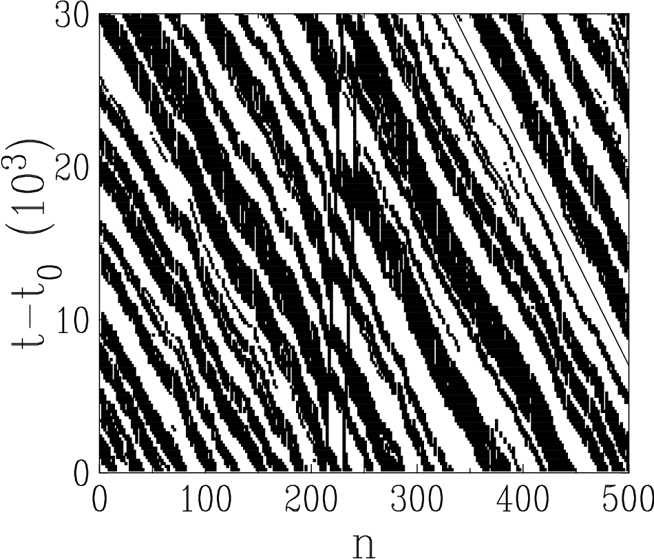
This scenario is confirmed by Figure 9, showing a space-time plot of the stationary dynamics of the domain pattern for . Equation (4.15) predicts , in reasonably good agreement with the observed value . The plot shows that the whole advected domain pattern behaves more or less as a rigid body over spatial scales much larger than the mean domain size .
5 Two-dimensional target process
We now consider the canonical target process defined by the rate (2.33), on the square lattice with unit vectors , . In order to have a genuine two-dimensional model and to maximize the asymmetry, we choose the following rule: particles hop either East (displacement ) or North (displacement ) with equal probabilities. In other words, if the departure site is , the arrival site is chosen to be either , or , with probability . The bias, i.e., the mean displacement proposed to a particle, , is along the North-East direction.
5.1 Heuristic argument
In the one-dimensional situation, the existence of a conserved current was instrumental in order to discriminate between possible scenarios for the stationary state of the model. In the present situation, however, the current is a two-dimensional vector. The condition that be conserved in the stationary state is less stringent than in the one-dimensional case. On spatial scales much larger than the lattice spacing, it is reasonable to use the continuum formalism. Within this framework, the conservation law reads . The symmetry of the dynamical rules implies that is aligned with the bias . Current lines are therefore parallel straight lines along this direction. The conservation law implies that the magnitude of the current is constant along each current line, but may well vary in the transversal direction from one current line to another. In particular the existence of an extended condensate is allowed, in the form of a one-dimensional structure elongated along the direction of the bias. This opens up the possibility of having an unconventional type of condensation transition. Such a phenomenon is indeed observed in the numerical simulations described hereafter.
5.2 Numerical results
We choose once for all the value in the numerical simulations of the two-dimensional target process defined above.
In analogy with the one-dimensional case, we begin with the transient dynamics, starting from a random initial condition. We monitor the local relaxation by means of the reduced second moment of the occupation distribution, introduced in (4.1). Figure 10 shows a plot of against time . For all values of the density , is an increasing function of time, starting from its initial value . The most significant feature to be observed on the data is the following: saturates to a finite limiting value, denoted , for values of the density up to the threshold value . We have for . To the contrary, grows indefinitely for larger values of the density. The right panel of Figure 10 demonstrates that the asymptotic growth law of for all is of the form
| (5.1) |
where is taken from the slope of the parallel dashed lines.


Pursuing along the lines of our investigation of the one-dimensional case, we introduce a local relaxation time , defined by the condition . Figure 11 shows a plot of so defined, divided by , against . The least-squares fit suggests a growth of the form (4.2), with , in a wide range of values of the density. Notice that the local relaxation time exhibits no visible singularity at the threshold density .

We now turn to a more accurate determination of the threshold density , using the pre-asymptotic growth of in the intermediate time regime, where has already departed in a significant way from its plateau value , but not yet reached the asymptotic linear growth (5.1). The right panel of Figure 10 demonstrates that this regime lasts longer and longer as the threshold density is approached. This observation is turned to a quantitative measurement by defining the global relaxation time by the condition , where we set , whereas the choice incorporates the form (5.1) of the asymptotic growth law. Figure 12 shows a plot of the reciprocal of the global time thus defined, against density. The data convincingly demonstrate that the global time diverges at some non-trivial threshold density . A crossover of the data toward another type of asymptotic behavior indeed seems extremely improbable, in view of the accuracy of the available data. The second-degree polynomial fit to the data shown on the plot provides a rather accurate determination of the threshold density,
| (5.2) |
as well as an evidence that the global time diverges linearly as the threshold density is approached from above, as
| (5.3) |
with a rather large prefactor .

The threshold density is the maximal density for which a homogeneous fluid phase is stable. At variance with the critical density of the symmetric target process and of the dual ZRP, rather appears as a dynamical threshold. This viewpoint is corroborated by the fact that the stationary state at density does not exhibit any critical feature. The distribution of the site occupations at the threshold density, shown in Figure 13, has an exponential fall-off of the form , with , at least in the accessible range of values of the occupation. We checked that the data are not affected in an appreciable way by finite-size effects in the range considered. The critical occupation distribution (2.41) of the dual ZRP is shown on the same plot as a comparison. The latter distribution has a much smaller density , some 12 times smaller than the observed threshold density (5.2) of the asymmetric two-dimensional model, but a slower power-law fall-off, so that the distributions eventually cross each other.

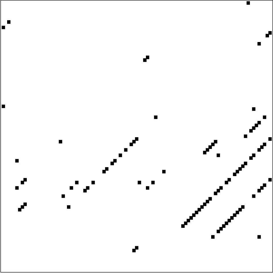
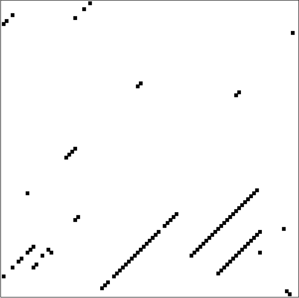
The progressive emergence of highly occupied coherent structures, which are strongly elongated along the direction of the bias, is illustrated in Figure 14, showing two snapshots of the coarsening regime of a sample of size at density . The filled symbols show the 1% most occupied sites. The visible structures clearly are precursors of the extended condensate mentioned above. The background density of the fluid phase besides these structures is found to be much smaller than the threshold density , and comparable to the critical density of the dual ZRP. We shall return to this point in more detail below (see Figure 16).
We now study the typical characteristic sizes (width and height) of the extended condensate in the stationary state of a finite system, and of its precursors in the coarsening regime of an infinite system. The width of a condensate is defined as the number of sites which take part in the condensate, whereas its height is the mean number of particles per site in the condensate, so that the product gives a measure of the number of particles involved in the condensate. We first consider the coarsening regime of an infinite system. The condensate precursors shown in Figure 14 are expected to be characterized by a typical width and height , with both scales growing with time. The contribution of these precursors to the reduced second moment of the occupation distribution can be checked to scale as , irrespective of the width . The growth law (5.1) therefore implies that the height of condensate precursors grows linearly in time, according to
| (5.4) |
with . This asymptotic coarsening law is expected to hold for any density . The behavior of the width of condensate precursors can only be investigated in an indirect way, by means of finite-size scaling. We therefore consider finite systems, namely square samples of linear size , with periodic boundary conditions. Figure 15 shows numerical data concerning the stationary state of finite systems against their linear size , at fixed density , well above the threshold density . The left panel shows the stationary-state value of the reduced second moment of the occupation distribution. The right panel shows the characteristic relaxation time , defined by the condition , again with . The data for both quantities clearly exhibit a linear growth with the size . The first of these growth laws implies . This is in accord with the expectation that typical stationary-state configurations have a single and roughly system-spanning extended condensate, for which . Furthermore, as the number of particles involved in the condensate scales as , we have . Let us now make the finite-size scaling assumption that and become respectively comparable to and for a time comparable to the relaxation time . This yields the scaling law , already known (see (5.4)), and the prediction .


Finally, we have also measured the background density of the fluid phase in the stationary state of finite samples at density . This quantity is algorithmically defined as follows. For any intercept , consider the total number of particles in the diagonal array with intercept , i.e., with equation :
| (5.5) |
The largest of these numbers, , corresponds to the diagonal array occupied by the extended condensate. It is overwhelmingly larger than the others, as it scales as . The other numbers represent the fluid phase, and therefore scale as . We are thus naturally led to define the background density as
| (5.6) |
where is the total number of particles in the system. Figure 16 shows a plot of the stationary-state background density for finite samples of size , against . The data demonstrate that is smaller than unity, and therefore much smaller than the mean density , as soon as . The segregation phenomenon is therefore already fully at work for rather small system sizes. From a quantitative viewpoint, a second-degree polynomial fit to the data yields the extrapolated value . The limiting value thus obtained is remarkable close to the critical density of the dual ZRP. Imposing the constraint indeed hardly changes the fit (dashed line). This agreement strongly suggests that the background fluid phase of the two-dimensional target process above its threshold density is characterized by the critical occupation distribution of the dual ZRP, just as the S-sites of the one-dimensional case in the high-density limit. As a consequence, the density of the fluid phase:
| (5.7) |
has a discontinuous jump at the threshold density .

6 Discussion
In this work we introduced a novel example of a migration process, the target process. We then studied in detail the structure of the nonequilibrium stationary state of the asymmetric target process, the main focus being on the fate of the condensation phenomenon.
The stationary-state measures of migration processes do not have a product form in general. The symmetric target process, though, has the same stationary-state product measure as the corresponding dual ZRP. In particular, the so-called canonical target process, defined by the rate (2.33) dual to the ZRP with rate (2.32), has a continuous condensation transition at a finite critical density whenever , with a macroscopic condensate occupying a single site for densities , irrespective of the dimensionality of the system. The asymmetric target process has a fluctuating stationary state with non-trivial spatial and temporal correlations, whose qualitative features depend on the dimensionality. Our main effort in the present work consisted in characterizing this nonequilibrium stationary state, including its dependence on the dimensionality.
We have reached a complete understanding of the one-dimensional target process, especially in the high-density regime of most interest. We showed, by exploiting the existence of a conserved current, that the asymmetric canonical target process has no condensation transition, and remains homogeneous at any finite density. In the high-density regime, an alternating scenario prevails for : typical configurations consist of long alternating sequences BSBSBSBS… of highly occupied B-sites, and less occupied S-sites, whose occupation distribution coincides with the critical distribution of the dual ZRP. The coherence length (mean domain size) of this alternating structure diverges as . We also gave a characterization of the scaling behavior of many other quantities in the vicinity of the ‘infinite-density fixed point’.
For the asymmetric target process in higher dimensions, we argued that the condensate must be extended and have the form of a one-dimensional structure elongated along the direction of the bias. In the two-dimensional case, numerical simulations performed for show that the model exhibits an unconventional condensation transition at the density . This density, which is much larger than the critical density of the dual ZRP, appears as a dynamical threshold: it is the maximal density at which a homogeneous fluid phase is dynamically stable. For , the predicted extended condensate is observed, whereas the background fluid phase again appears as critical. This picture seems to be generic for higher-dimensional systems. Preliminary numerical simulations of the asymmetric target process on the three-dimensional cubic lattice (where the displacement is along either of the unit vectors , , with equal probabilities), indeed show that the overall picture is quite similar to the two-dimensional one. The global relaxation time is again found to diverge according to (5.3), with for .
Let us mention that another mechanism leading to an extended condensate in a class of mass transport models in one dimension has been reported recently [20]. There, the nonequilibrium stationary-state measure is a product whose factors involve the occupations of two consecutive sites. In the condensed phase, those models exhibit an extended condensate, whose height and width scale as for a finite system of sites. These scaling laws are formally identical to those found in the present work.
The existence of a threshold density at which the background density has a discontinuous jump (see (5.7)) is reminiscent of what occurs in the model studied in [21], namely a ZRP with two species of particles, and with rates such that the stationary-state measure does not have a product form. When the densities and of the two species are equal, the behavior of the system is qualitatively the same as that of the canonical ZRP (with one species). In particular the system has a continuous phase transition at some critical density , from a fluid phase to a condensed phase with critical background. The general situation where the two densities are different however drastically departs from this known scenario. If either of the two densities (, say) is kept fixed at a value larger than , on increasing the other density , the system remains homogeneous as long as is less than a threshold value which depends on . At this threshold the system undergoes a discontinuous transition from an imbalanced fluid phase, where both species have densities and larger than the critical density, to an imbalanced condensate coexisting with a balanced critical fluid with densities .
Finally, the observed rapid growth of the threshold density with the dimensionality raises the question of the behavior of the asymmetric target process in high dimensions. At this point let us emphasize that the absence of a stationary-state product measure for the target process is a rather subtle effect which needs the conjunction of several ingredients, and chiefly the presence of a bias. This feature cannot be present in mean-field geometries such as the complete graph, so that the dynamical threshold behavior of the model in high dimensions is not expected to smoothly converge to a well-defined mean-field limit.
References
References
- [1] O’Loan O J, Evans M R and Cates M E, 1998 Phys. Rev. E 58 1404
- [2] Evans M R, 2000 Braz. J. Phys. 30 42
- [3] Kafri Y, Levine E, Mukamel D, Schütz G M and Török J, 2002 Phys. Rev. Lett. 89 035702
- [4] Godrèche C, 2003 J. Phys. A 36 6313
- [5] Grosskinsky S, Schütz G M and Spohn H, 2003 J. Stat. Phys. 113 389
- [6] Evans M R and Hanney T, 2005 J. Phys. A 38 R195
- [7] Godrèche C and Luck J M, 2005 J. Phys. A 38 7215
- [8] Bialas P, Burda Z and Johnston D, 1997 Nucl. Phys. B 493 505 Bialas P, Burda Z and Johnston D, 1999 Nucl. Phys. B 542 413 Bialas P, Bogacz L, Burda Z and Johnston D, 2000 Nucl. Phys. B 575 599
- [9] Drouffe J M, Godrèche C and Camia F, 1998 J. Phys. A 31 L19
- [10] Godrèche C and Luck J M, 2001 Eur. Phys. J. B 23 473
- [11] Godrèche C and Luck J M, 2002 J. Phys. Cond. Matt. 14 1601
- [12] Godrèche C, 2007 Lect. Notes Phys. 716 216 (Berlin: Springer) (cond-mat/0604276)
- [13] Majumdar S N, Evans M R and Zia R K P, 2005 Phys. Rev. Lett. 94 180601 Evans M R, Majumdar S N and Zia R K P, 2006 J. Stat. Phys. 123 357
- [14] Spitzer F, 1970 Advances in Math. 5 246
- [15] Andjel E D, 1982 Ann. Prob. 10 525
- [16] Kelly F, 1979 Reversibility and Stochastic Networks (Chichester: Wiley)
- [17] Cocozza-Thivent C, 1985 Z. Wahr. 70 509
- [18] Schütz G M, Ramaswamy R and Barma M, 1996 J. Phys. A 29 837
- [19] Luck J M and Godrèche C, 2006 J. Stat. Mech. P08009
- [20] Evans M R, Hanney T and Majumdar S N, 2006 Phys. Rev. Lett. 97 010602
- [21] Godrèche C, 2006 J. Phys. A 39 9055