Plastic response of a 2d amorphous solid to quasi-static shear :
I - Transverse particle diffusion and phenomenology of dissipative events

We use here the same binary LJ mixture as that of ref.MaloneyLemaitre2006, namely large (L) and small(S) particle radii and numbers are: $r_{L}=0.5$, $r_{S}=0.3$, and $N_{L}=N_{S}(1+\sqrt{5})/4$. These values ensure that no crystallization occurs at low temperature. Simple shear deformation is imposed using Lees-Edwards boundary conditions. We study systems of three different sizes $L\times L$, with $L=10,20,40$.

The quasi-static regime corresponds to the limit where the external time scale $\dot{\gamma}^{-1}$ is much larger than that of internal relaxation processes. The system, starting from local equilibrium, thus follows adiabatically the shear-induced evolution of the corresponding energy minimum up to the spinodal limit where this minimum disappears and the system jumps into another local minimum of lower energy. The simulation proceeds as follows: a small increment $\delta$ of homogeneous shear strain is imposed, then energy is minimized using a conjugate gradient algorithm with a stringent convergence criterion (see MaloneyLemaitre2006 for details). We choose $\delta=10^{-4}$, small enough to ensure that, for our system sizes, all elastic branches are well resolved. A typical $\sigma(\gamma)$ curve is displayed on Figure 1.

Starting from an initial quench, we explore the shear range $\gamma\leq 2$. In order to characterize the stationary state, we only retain data for $\gamma>0.1$, which ensures that initial transients are discarded, thus making details of the quenching protocol immaterial. We have been able to collect data on $100$, $50$ and $20$ systems of respective sizes $L=10,20,40$.

Following ref.MaloneyLemaitre2006, we make extensive use of the so-called non-affine tangent field $\{\bf{u}_{i}\}$, defined as the difference between the linear response of particle displacements to an increment of homogeneous strain and the corresponding homogeneous field. It is well-defined, and is computed, everywhere along each elastic branch.

In plastically deforming amorphous systems, non-affine displacement fields contain information about both, departures from standard continuum elastic behavior and the nature of plastic events. In our simple shear geometry, transverse particle displacements $\Delta y_{i}$ are purely non-affine, while longitudinal ones mix affine and non-affine contributions. We thus focus on the normalized distributions $P(\Delta y,\Delta\gamma)$ of the $\Delta y_{i}$’s for a fixed strain interval $\Delta\gamma$. The statistical ensemble is built by sampling, for all initial configurations, all the $\Delta y_{i}=y_{i}(\gamma_{0}+\Delta\gamma)-y_{i}(\gamma_{0})$ at each step $\gamma_{0}$ ($0.1\leq\gamma_{0}\leq 2-\Delta\gamma$).

Our results agree qualitatively with those of Tanguy et al TanguyLeonforteBarrat2006. Namely (see Figure 2) $P(\Delta y,\delta)$ has a quasi-gaussian center and exhibits, beyond $\Delta y\sim 0.2$, an exponential tail. Its fine structure shows more clearly in the log-lin representation of the distribution $\tilde{P}(\zeta)$ of the scale variable $\zeta={\rm log}(\Delta y)$. As displayed on Figure 3, for small strain intervals ($\Delta\gamma/\delta\sim$ a few units), the corresponding curves exhibit a peak at small $\Delta y$ in the $10^{-4}$ range, together with a broad hump for larger values. As $\Delta\gamma$ increases, the peak shifts to the right and the hump amplitude grows, though without noticeable horizontal shift, until both merge, for $\Delta\gamma\approx 10^{-2}$.

Can we interpret this structure and its evolution in the light of the succession of elastic and plastic episodes which reflect into the sawtooth shape of the $\sigma(\gamma)$ response? Clearly, particle motion consists of a series of continuous trajectories interrupted by sudden jumps associated, respectively, with elastic episodes and plastic events. Since $\delta$ is our numerical strain resolution, each interval of length $\delta$ is, within our accuracy, defined as either purely elastic or purely plastic. So, for $\Delta\gamma=\delta$, we can decompose $P$ (and likewise $\tilde{P}$) as :

where $\alpha_{pl}(\delta)$ is the fraction of ”plastic intervals” in our ensemble, and $\Pi_{pl}$ (resp. $\Pi_{el}$) are the normalized distributions associated with the plastic (resp. elastic) sub-ensemble. It now clearly appears (see Figure 4) that the small $\Delta y$ behavior of $P(\Delta y,\delta)$ results entirely from elastic motion, while its hump and large-$\Delta y$ tail are due to plastic events.

On this basis, we are now able to understand the evolution of $\tilde{P}$ with $\Delta\gamma$. We extend the above decomposition to $\Delta\gamma>\delta$, now defining as ”plastic” any interval containing at least one plastic event. As $\Delta\gamma$ increases while remaining small with respect to the average length ($\delta\alpha_{pl}(\delta)^{-1})$) of an elastic branch, most plastic intervals in general still contain only one plastic event, so that their fraction $\alpha_{pl}(\Delta\gamma)\approx(\Delta\gamma/\delta)\alpha_{pl}(\delta)$, while $\Pi_{pl}$ remains quasi unchanged, because the scale of plastic slips is large compared with that of elastic ones. This explains the evolution (Figure 4) of the plastic hump which, as $\Delta\gamma$ increases, consists primarily in an upward shift with little change in shape.

In this regime, which corresponds to $\Delta\gamma/\delta<<\alpha_{pl}(\delta)^{-1}$ ( $\sim 100$ for the $20\times 20$ system), the fraction $\alpha_{el}=(1-\alpha_{pl})$ of purely elastic intervals remains nearly constant (e.g., for $L=20$ and $\Delta\gamma=10\delta$, $\delta\alpha_{el}/\alpha_{el}\sim 0.1$), so that the variations with $\Delta\gamma$ of the elastic part of $\tilde{P}$, $\tilde{P}_{el}=\alpha_{el}(\Delta\gamma)\tilde{\Pi}_{el}$, directly reveal those of $\tilde{\Pi}_{el}$. Inspection of the numerical data suggests (see also Figure 4) that the rightward shifts of $\tilde{P}_{el}(\zeta)$ are roughly equal to ${\rm log}(\Delta\gamma)$. The plot (Figure 5) of $\tilde{P}_{el}$ vs $\log(\Delta y/\Delta\gamma$)) shows that the collapse is indeed excellent in the low and middle ranges of $(\Delta y/\Delta\gamma)$ values, but fails in the large $\Delta y$ tails.

This collapse means that during the purely elastic episodes separating plastic events non-affine displacements are essentially convective: the $\gamma$-derivative of the $y_{i}$ field is nearly constant over most of an elastic episode. This amounts to stating that the tangent non-affine field $\{\bf{u}_{i}\}$, although spatially disordered footnote, remains quasi-quenched. Now, we know from ref. MaloneyLemaitre2004a that this cannot be true when the system comes close below a spinodal threshold $\gamma_{c}$. Indeed, in these near-critical regions, a gradually softening elastic mode develops, leading to a $(\gamma_{c}-\gamma)^{-1/2}$ divergence of $\{\bf{u}_{i}\}$. Clearly, it is the contribution of these near-critical softened configurations which explains the large-$\Delta y$ tails of $\tilde{\Pi}_{el}$. The tail deflation (Figure 5) results from the fact that, as the interval $\Delta\gamma$ increases, the weight of these soft configurations is gradually transferred from $\tilde{\Pi}_{el}$ to $\tilde{\Pi}_{pl}$.

This analysis clarifies the physical significance of the shape of $P(\Delta y,\Delta\gamma)$ in the moderate $\Delta\gamma$ range (where its non-Gaussian parameter remains large TanguyLeonforteBarrat2006): (i) Its quasi-gaussian center footnote results from small-scale non-affine displacements accumulated along purely elastic segments, during which particle trajectories are essentially convected. (ii) Its quasi-exponential tail arises from plastic jumps during plastic events.

For larger $\Delta\gamma/\delta\gtrsim\alpha_{pl}(\delta)^{-1}$, however, the decomposition of equation (1) loses physical content since the statistical weight of elastic intervals vanishes while $\tilde{\Pi}_{pl}$ mixes both elastic and plastic contributions. In order to circumvent this limitation, we concentrate in the following on the evolution with $\Delta\gamma$ of the second moment $\langle\Delta y^{2}\rangle$.

In order to elucidate the nature of the transverse particule dynamics, we have computed from our data the space and ensemble average $\langle\Delta y^{2}\rangle$ for increasing values of $\Delta\gamma$. On Figure 6 we plot the effective diffusion coefficient $D(\Delta\gamma)=\langle\Delta y^{2}\rangle/\Delta\gamma$. For our three system sizes, $D(\Delta\gamma)$ exhibits the same qualitative features, namely it increases from a finite value $D_{0}=\lim\limits_{\Delta\gamma\to 0}D$, and saturates at a finite value $D_{\infty}$ for large $\Delta\gamma$ ($\gtrsim 0.5$). However, $D$ is strikingly system-size dependent, $D^{(L)}(\Delta\gamma)$ increasing with $L$ for all $\Delta\gamma$’s.

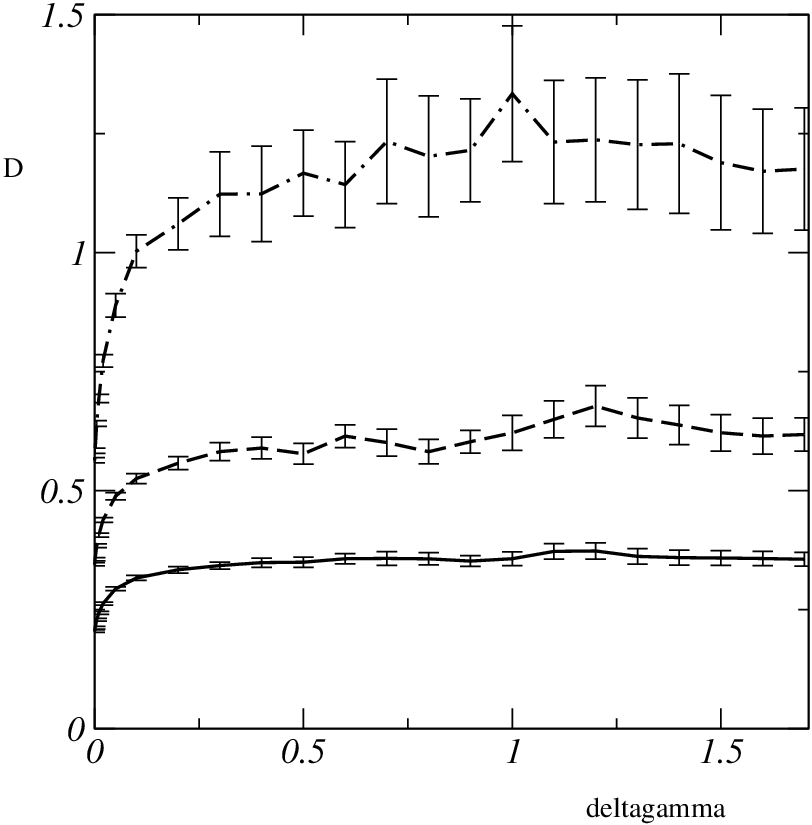
Again, in order to shed light on the origin of this behavior, let us separate explicitly the elastic and plastic contributions to non-affine particle motion. Indeed, we can write:

where $a$ labels the strain values where irreversible events (avalanches) occur, so that :

with

and $D_{ep}$, $D_{pp}$ the corresponding cross-correlated and plastic-plastic contributions. These three functions carry the information about self and cross correlations of elastic and plastic non-affine displacements.

Let us first consider the $\Delta\gamma\to 0$ limit. A straightforward asymptotic analysis taking into account the square-root divergence of the tangent field $\{\bf{u}_{i}(\gamma)\}$ at spinodal points leads to:

So, their contribution to $D(\Delta\gamma)$ vanishes, and the finite value of $D_{0}$ originates only from avalanches:

with

the average avalanche frequency, and $\langle\left(Y_{i}^{a})^{2}\right)\rangle$ the variance of transverse displacements in a single plastic event.

It was shown in MaloneyLemaitre2004; MaloneyLemaitre2006 that $f$ increases with size roughly as the lateral system size $L$. Using the measured frequency, we find that the variance $\langle\left(Y_{i}^{a})^{2}\right)\rangle=D_{0}f^{-1}$ decreases slowly with size: for $L=10,20,40$, we get $10^{4}\langle\left(Y_{i}^{a})^{2}\right)\rangle=37,26,20$. We will come back to this point later.

Figure 7 shows the decomposition (eq.(3)) for $L=20$. It is seen that, for all $\Delta\gamma$, $D_{pp}$ remains the dominant contribution. $D_{pp}(\Delta\gamma)$ grows, then saturates. Its growth range $\Gamma_{pp}\sim 0.25$ shows no clear size dependence. This behavior entails that plastic events are correlated over a finite $\Delta\gamma$ range, which we understand as measuring a typical shear range over which the structural features involved in plastic events retain their identity.

For all sizes, $D_{ep}(\Delta\gamma)$, though much smaller than $D_{pp}$, exhibits an analogous behavior with a similar correlation range. This indicates that the above-mentioned persistent structures dominate the non-affine elastic response. Moreover the near square-root behavior footnote2 of $D_{ep}$ for small $\Delta\gamma$ signals that the field $\{\bf{u}_{i}\}$ in a given near-critical region is strongly correlated with the displacements associated with the subsequent avalanche.

Finally, $D_{ee}$ also rises and saturates, but more slowly than $D_{ep}$ and $D_{pp}$. From the data for the three system sizes, we evaluate its correlation range to be $\Gamma_{ee}\sim 1$. That is, a single renewal, after $\Delta\gamma\sim\Gamma_{pp}$, of the ”active structures” is not sufficient for the non-affine field to fully decorrelate. This we take as a hint of the fact that active structures occupy on average a fraction only of the total system ”volume”. With this interpretation, we evaluate this fraction as $\Gamma_{pp}/\Gamma_{ee}\sim 1/4$.

Let us first recall that $\{\bf{u}_{i}\}$ can be written as MaloneyLemaitre2004a:

where $(i,j)$ label particles and $(\alpha,\beta)$ cartesian components. $U$ is the total energy of the LJ system, and $\bar{\bar{H}}$ the associated hessian matrix. $\bf{\Xi}\delta\gamma$ is the field of particle force increments generated by an infinitesimal increment of homogeneous shear. $\{\bf{u}_{i}\}$ can be decomposed on the eigenmodes $\bf{\Psi}_{n}$ of $\bar{\bar{H}}$ (the phonon modes). Upon approaching a spinodal point, a single one, $\bf{\Psi}_{1}$, softens critically MalandroLacks1999; MaloneyLemaitre2004a. So, in near critical regions, $\{\bf{u}_{i}\}$ exhibits a square-root divergence and is dominated by its projection $\bf{u}_{1}$ on $\bf{\Psi}_{1}$. This property enables us to clearly characterize the active structures close to the onset of plastic events.

The features we identify as characteristic of the evolution of $\{\bf{u}\}$ are exemplified on Figures 8 and 9. In these figures, for each value of $\gamma$ we decompose the total non-affine field as:

with $\bf{u}_{1,2}$ its projections on the two modes $\bf{\Psi}_{1,2}$ with lowest eigenvalues ($\lambda_{1}<\lambda_{2}$).

We observe that, in all cases, the active structures emerge out of a quasi-random small background as one or several localized zones characterized by strong quadrupolar contributions to $\bf{u}$. These quadrupoles are approximately aligned with the principal directions of the homogeneous strain. As zones approach instability, they soften, and the corresponding growing part of $\bf{u}$ concentrates into the lowest mode component $\bf{u}_{1}$.

After identifying them in prespinodal regions, we are able to trace them back over sizeable $\gamma$-ranges before their amplitude has decreased enough for them to gradually merge into the global disordered background structures. In some cases, this range of visibility extends across one or more plastic events. A typical sequence illustrating this behavior, shown on Figure 8, extends over a range of $\Delta\gamma\sim 3\%$, to be compared with the average length $\Delta\gamma\sim 1\%$ of elastic episodes for this system size.

Each discontinuous drop on the $\sigma(\gamma)$ curve is associated with the sudden disappearance of one or more of these soft zones (Figures 8 and 9). Noticeably, the resulting changes in $\{\bf{u}_{i}\}$ remain quite localized, leaving most of the other prominent structures of the non-affine pattern essentially unchanged. In particular, zones which were already clearly visible are commonly seen to survive the plastic event (see Figure 8).

We have shown in Section II.2 that particle jumps $\{\Delta\bf{R}_{i}^{a}\}$ in plastic events are well correlated with the precritical $\{\bf{u}_{i}\}$ structure. This entails that the flip of a zone Z is associated primarily with a quadrupolar displacement field of finite amplitude centered on Z. This supports the representation, proposed by Argon and coworkers BulatovArgon1994a; ArgonBulatovMottSuter1995 and explicited by Picard et al PicardAjdariLequeuxBocquet2004, of the elementary dissipative process as the Eshelby-like shear transformation of a self generated inclusion involving a few particles, which is also the basis of the STZ theory.

This representation is also consistent with the main features of the distribution $\Pi_{pl}(\Delta y,\delta)$ of particle displacements induced by plastic events (see $\lx@sectionsign$ II.B). Indeed, the plot on Figure 10 shows that that $\Pi_{pl}$ becomes exponential for $\Delta y\gtrsim 0.2$. In the Eshelby picture, we expect large $\Delta y$ to correspond to displacements within the transforming zone(s), while smaller $\Delta y$ are associated with particles sitting in the surrounding elastic medium. In this picture, we interpret the exponential tail of $\Pi_{el}$, hence of the full distribution $P$, as reflecting the diversity of intrazone structures. We thus expect that, upon varying the system size, the logarithmic slope of the tail should remain constant. As shown on Figure 10, this prediction is very nicely verified for our three $L$ values. Moreover, it appears that the tail amplitude decreases with increasing $L$. In our interpretation, the statistical weight of the exponential tail is controlled by the volume fraction of zone cores involved in plastic events. Since the average size of the avalanches constituting plastic events scales roughly as $L$, we expect the corresponding core volume fraction to decrease with size, in agreement with the observed behavior.

So, we interpret the existence of an exponential tail in $P(\Delta y)$ as a consequence of structural disorder within transforming zones, and by no means as a signature of avalanche behavior, which only affects the tail amplitude.

Consider the sequence shown on Figure 9. For $\gamma=0.1150$ (Figure 9-a) two zones are clearly discernible in the $\bf{u}$ pattern. At $\gamma=0.1160$ (Figure 9-b) their amplitude has grown, and they appear in the projection $\bf{u}_{2}$ of $\bf{u}$ on the next-to-lowest mode. At $\gamma=0.1161$ (Figure 9-c) they are slightly softer and have invaded the projection $\bf{u}_{1}$ on the lowest mode. Note that, in these last two cases, they appear in the non-trivial soft mode as connected by ”flow lines” which reproduce the most prominent vortex structures first described by Tanguy et al TanguyWittmerLeonforteBarrat2002. This is particularly clear when two relatively distant zones soften simultaneously as shown on Figure 11.

From these and many similar observations (see Figure 8) we deduce that :

$\bullet$ Soft zones are coupled elastically via their quadrupolar fields.

$\bullet$ It is the associated flow lines which form the conspicuous vortex-like patterns characteristic of non-affine fields in amorphous solids. That such patterns are akin to incompressible flows results from the fact that these systems are much more compliant in shear than in compression. For our 2D LJ glass MaloneyLemaitre2006: $\mu=39$, $K=236$.

Quadrupolar couplings result, in the homogeneous elastic continuum approximation for the background medium, from a stress field $\sim{\rm cos}(4\theta)/R^{2}$ (with $R$ the length and $\theta$ the orientation with respect to $\hat{x}$ of the interzone vector). Notice that, in Figure 9, in $\bf{u}_{1}$ the fields of the two zones $Z_{1}$, $Z_{2}$, which are quasi vertically aligned, combine positively. We have checked that, in consistence with the above remark, zone pairs lying in sectors corresponding to negative couplings combine negatively in the phonons $\bf{\Psi}_{1}$ and $\bf{\Psi}_{2}$: in this case, one of the two zones appears with an opposite sign, i.e. with reversed flow lines. These observations confirm the relevance of inter-zone elastic couplings.

It is intuitively clear that configurations with strongly coupled soft zones are good candidates for simultaneous flips, as illustrated on Figure 8 and 9. We observe a number of multi-zone flips, involving the disappearance of at least one diverging quadrupole, as well as that of some less visible zones. Moreover, plastic events alter the amplitude of the near-critical surviving zones in $\bf{u}$ (see Figure 8) in a way which appears roughly consistent with quadrupolar couplings.

References

- (1) S. Kobayashi, K. Maeda, and S. Takeuchi, Acta Met 28, 1641 (1980).
- (2) D. Deng, A. S. Argon, and S. Yip, Philos. Trans. R. Soc. Lond. Ser. A-Math. Phys. Eng. Sci. 329, 549 (1989).
- (3) A. S. Argon, V. V. Bulatov, P. H. Mott, and U. W. Suter, J. Rheol. 39, 377 (1995).
- (4) C. Maloney and A. Lemaître, Phys. Rev. E 74, 016118 (2006).
- (5) N. Bailey, J. Schiøtz, A. Lemaître, and K. Jakobsen, Phys. Rev. Lett. 98, 095501 (2007).
- (6) J. D. Eshelby, Proc. Roy. Soc. London A 241, 376 (1957).
- (7) G. Picard, A. Ajdari, F. Lequeux, and L. Bocquet, Eur. Phys. J. E 15, 371 (2004).
- (8) V. V. Bulatov and A. S. Argon, Model. Simul. Mater. Sci. Eng. 2, 167 (1994).
- (9) M. L. Falk and J. S. Langer, Phys. Rev. E 57, 7192 (1998).
- (10) A. Tanguy, F. Leonforte, and J.-L. Barrat, cond-mat/0605397, 2006.
- (11) Note that the position of the peak of corresponds, roughly, to the width of the gaussian approximant of the small- part of .
- (12) M. J. Demkowicz and A. S. Argon, Physical Review B 72, 245206 (2005).
- (13) C. Maloney and A. Lemaître, Phys. Rev. Lett. 93, 16001 (2004).
- (14) C. Maloney and A. Lemaître, Phys. Rev. Lett. 93, 195501 (2004).
- (15) Strictly speaking, in order to observe the asymptotic behavior, we would need data for decreasing simulation strain intervals . With our value , we measure at small an effective behavior .
- (16) M. L. Falk and J. S. Langer, M.R.S. Bulletin 25, 40 (2000).
- (17) P. Sollich, F. Lequeux, P. Hébraud, and M. E. Cates, Phys. Rev. Lett. 78, 2020 (1997).
- (18) P. Sollich, Phys. Rev. E 58, 738 (1998).
- (19) D. L. Malandro and D. J. Lacks, J. Chem. Phys. 110, 4593 (1999).
- (20) A. Tanguy, J. P. Wittmer, F. Leonforte, and J.-L. Barrat, Phys. Rev. B 66, 174205 (2002).
- (21) G. Picard, A. Ajdari, F. Lequeux, and L. Bocquet, Phy. Rev. E 71, 010501 (2005).
- (22) J. C. Baret, D. Vandembroucq, and S. Roux, Phys. Rev. Lett. 89, 195506 (2002).
- (23) B. Doliwa and A. Heuer, Physical Review E 67, 031506 (2003).
- (24) B. Doliwa and A. Heuer, Physical Review E 67, 030501 (2003).
- (25) B. Doliwa and A. Heuer, Physical Review Letters 91, 235501 (2003).
- (26) T. B. Schrøder, S. Sastry, J. C. Dyre, and S. C. Glotzer, jcp 112, 9834 (2000).
- (27) M. Goldstein, J. Chem. Phys. 51, 3728 (1969).
- (28) A. Widmer-Cooper and P. Harrowell, Journal of Physics: Condensed Matter 17, S4025 (2005).
- (29) A. Widmer-Cooper and P. Harrowell, Physical Review Letters 96, 185701 (2006).