¹¹ 1 Supported in part at the Technion by a fellowship of the Israel Council for Higher Education

Algorithmic Problems in Amalgams of Finite Groups

L.Markus-Epstein Address: Department of Mathematics
Technion
Haifa 32000, Israel Email address: epstin@math.biu.ac.il

Abstract.

Geometric methods proposed by Stallings [54] for treating finitely generated subgroups of free groups were successfully used to solve a wide collection of decision problems for free groups and their subgroups [5, 26, 38, 39, 44, 49, 57].

It turns out that Stallings’ methods can be effectively generalized for the class of amalgams of finite groups [40]. In the present paper we employ subgroup graphs constructed by the generalized Stallings’ folding algorithm, presented in [40], to solve various algorithmic problems in amalgams of finite groups.

1. Introduction

Decision (or algorithmic) problems is one of the classical subjects of combinatorial group theory, originating in the three fundamental decision problems posed by Dehn [12] in 1911: the word problem (which asks to answer whether a word over the group generators represents the identity), the conjugacy problem (which asks to answer whether an arbitrary pair of words over the group generators define conjugate elements) and the isomorphism problem (which asks to answer whether an arbitrary pair of finite presentations determine isomorphic groups).

Though Dehn solved all three of these problems as restricted to the canonical presentation of fundamental groups of closed 2-manifolds, they are theoretically undecidable (unsolvable) in general [45, 46]. However restrictions to some particular classes of groups may yield surprisingly good results. Remarkable examples include the solvability of the word problem in one-relator groups (Magnus, see II.5.4 in [36]) and in hyperbolic groups (Gromov, see 2.3.B in [18]). The reader is referred to the papers of Miller [45, 46] for a survey of decision problems for groups.

The groups considered in the present paper are amalgams of finite groups. As is well known [3], these groups are hyperbolic. Therefore the word problem in this class of groups is solvable. A natural generalization of the word problem is the (subgroup) membership problem (or the generalized word problem), which asks to decide whether a word in the generators of the group is an element of the given subgroup. An efficient solution of the membership problem in amalgams of finite groups was presented by the author in [40], where graph theoretic methods for treating amalgams of finite groups were developed. Namely, a finitely generated subgroup $H$ of an amalgam $G=G_{1}\ast_{A}G_{2}$ of finite groups is canonically represented by a finite labelled graph $\Gamma(H)$ . This graph carries all the essential information about the subgroup $H$ itself, which enables one to “read off” a solution of the membership problem in $H$ directly from its subgroup graph $\Gamma(H)$ . This yields a quadratic (and sometimes even linear) time solution of the membership problem in amalgams of finite groups.

Such strategy was originally developed by Stallings [54] to treat finitely generated subgroups of free groups. Stallings’ approach was topological. He showed that every finitely generated subgroup of a free group is canonically represented by a minimal immersion of a bouquet of circles. Using the graph theoretic language, the results of [54] can be restated as follows. A finitely generated subgroup of a free group is canonically represented by a finite labelled graph which can be constructed algorithmically by a so called process of Stallings’ foldings (Stallings’ folding algorithm). Moreover, this algorithm is quadratic in the size of the input [26, 39]. See [56] for a faster implementation of this algorithm.

In [40] Stallings’ folding algorithm was generalized to the class of amalgams of finite groups. Along the current paper we refer to this algorithm as the generalized Stallings’ folding algorithm. Its description is included in the Appendix.

Note that graphs constructed by the Stallings’ folding algorithm can be viewed as finite inverse automata as well. This convergence of ideas from the group theory, topology, graph theory, the theory of finite automata and finite semigroups yields reach computational and algorithmic results concerning free groups and their subgroups. In particular, this approach gives polynomial time algorithms to solve the membership problem, the finite index problem, to compute closures of subgroups in various profinite topologies. See [5, 38, 39, 44, 49, 57] for these and other examples of the applications of the Stallings’ approach in free groups, and [29, 30, 43, 51] for the applications in some other classes of groups. Note that the Stallings’ ideas were recast in a combinatorial graph theoretic way in the remarkable survey paper of Kapovich and Myasnikov [26], where these methods were applied systematically to study the subgroup structure of free groups.

Our objective is to apply the generalized Stallings’ methods developed by the author in [40] to solve various decision problems concerning finitely generated subgroups of amalgams of finite groups algorithmically (that is to find a precise procedure, an algorithm), which extends the results of [26].

Our results include polynomial solutions for the following algorithmic problems in amalgams of finite groups, which are known to be unsolvable in general [45, 46]:

•

computing subgroup presentations,
•

detecting triviality of a given subgroup,
•

the freeness problem,
•

the finite index problem,
•

the separability problem,
•

the conjugacy problem,
•

the normality,
•

the intersection problem,
•

the malnormality problem,
•

the power problem,
•

reading off Kurosh decomposition for finitely generated subgroups of free products of finite groups.

These results are spread out between three papers: [41, 42] and the current one. In [42] free products of finite groups are considered, and an efficient procedure to read off a Kurosh decomposition is presented.

The splitting between [41] and the current paper was done with the following idea in mind. It turn out that some subgroup properties, such as computing of a subgroup presentation and index, as well as detecting of freeness and normality, can be obtained directly by an analysis of the corresponding subgroup graph. Solutions of others require some additional constructions. Thus, for example, intersection properties can be examined via product graphs, and separability needs constructions of a pushout of graphs.

In the current paper algorithmic problems of the first type are presented: the computing of subgroup presentations, the freeness problem and the finite index problem. The separability problem is also included here, because it is closely related with the other problems presented in the current paper. The rest of the algorithmic problems are introduced in [41].

The paper is organized as follows. The Preliminary Section includes the description of the basic notions used along the present paper. Readers familiar with amalgams, normal words in amalgams and labelled graphs can skip it. The next section presents a summary of the results from [40] which are essential for our algorithmic purposes. It describes the nature and the properties of the subgroup graphs constructed by the generalized Stallings’ folding algorithm in [40]. The rest of the sections are titled by the names of various algorithmic problems and present definitions (descriptions) and solutions of the corresponding algorithmic problems. The relevant references to other papers considering similar problems and a rough analysis of the complexity of the presented solutions (algorithms) are provided. In contrast with papers that establish the exploration of the complexity of decision problems as their main goal (for instance, [27, 28, 56]), we do it rapidly (sketchy) viewing in its analysis a way to emphasize the effectiveness of our methods.

Other Methods

There have been a number of papers, where methods, not based on Stallings’ foldings, have been presented. One can use these methods to treat finitely generated subgroups of amalgams of finite groups. A topological approach can be found in works of Bogopolskii [6, 7]. For the automata theoretic approach, see papers of Holt and Hurt [24, 25], papers of Cremanns, Kuhn, Madlener and Otto [11, 31], as well as the recent paper of Lohrey and Senizergues [32].

However the methods for treating finitely generated subgroups presented in the above papers were applied to some particular subgroup property. No one of these papers has as its goal a solution of various algorithmic problems, which we consider as our primary aim. Moreover, similarly to the case of free groups (see [26]), our combinatorial approach seems to be the most natural one for this purpose.

2. Acknowledgments

I wish to deeply thank to my PhD advisor Prof. Stuart W. Margolis for introducing me to this subject, for his help and encouragement throughout my work on the thesis. I owe gratitude to Prof. Arye Juhasz for his suggestions and many useful comments during the writing of this paper. I gratefully acknowledge a partial support at the Technion by a fellowship of the Israel Council for Higher Education.

3. Preliminaries

Amalgams

Let $G=G_{1}\ast_{A}G_{2}$ be a free product of $G_{1}$ and $G_{2}$ with amalgamation, customary, an amalgam of $G_{1}$ and $G_{2}$ . We assume that the (free) factors are given by the finite group presentations

(

1.a

)

\displaystyle G_{1}=gp\langle X_{1}|R_{1}\rangle,\ \ G_{2}=gp\langle X_{2}|R_{2}\rangle\ \ {\rm such\ that}\ \ X_{1}^{\pm}\cap X_{2}^{\pm}=\emptyset.

$A=\langle Y\rangle$ is a group such that there exist two monomorphisms

(

1.b

)

\displaystyle\phi_{1}:A\rightarrow G_{1}\ {\rm and}\ \phi_{2}:A\rightarrow G_{2}.

Thus $G$ has a finite group presentation

(

1.c

)

\displaystyle G=gp\langle X_{1},X_{2}|R_{1},R_{2},\phi_{1}(a)=\phi_{2}(a),\;a\in Y\rangle.

We put $X=X_{1}\cup X_{2}$ , $R=R_{1}\cup R_{2}\cup\{\phi_{1}(a)=\phi_{2}(a)\;|\;a\in Y\}$ . Thus $G=gp\langle X|R\rangle$ .

As is well known [36, 37, 52], the free factors embed in $G$ . It enables us to identify $A$ with its monomorphic image in each one of the free factors. Sometimes in order to make the context clear we use $G_{i}\cap A$ ²² 2 Boxes are used for emphasizing purposes only. to denote the monomorphic image of $A$ in $G_{i}$ ( $i\in\{1,2\}$ ).

Elements of $G=gp\langle X|R\rangle$ are equivalence classes of words. However it is customary to blur the distinction between a word $u$ and the equivalence class containing $u$ . We will distinguish between them by using different equality signs: “ $\equiv$ ” for the equality of two words and “ $=_{G}$ ” to denote the equality of two elements of $G$ , that is the equality of two equivalence classes. Thus in $G=gp\langle x\;|\;x^{4}\rangle$ , for example, $x\equiv x$ but $x\not\equiv x^{-3}$ , while $x=_{G}x^{-3}$ .

Normal Forms

Let $G=G_{1}\ast_{A}G_{2}$ . A word $g_{1}g_{2}\cdots g_{n}\in G$ is in normal form (or, simply, it is a normal word) if:

(1)

$g_{i}\neq_{G}1$ lies in one of the factors, $G_{1}$ or $G_{2}$ ,
(2)

$g_{i}$ and $g_{i+1}$ are in different factors,
(3)

if $n\neq 1$ , then $g_{i}\not\in A$ .

We call the sequence $(g_{1},g_{2},\ldots,g_{n})$ a normal decomposition of the element $g\in G$ , where $g=_{G}g_{1}g_{2}\cdots g_{n}$ .

Any $g\in G$ has a representative in a normal form (see, for instance, p.187 in [36]). If $g\equiv g_{1}g_{2}\cdots g_{n}$ is in normal form and $n>1$ , then the Normal Form Theorem (IV.2.6 in [36]) implies that $g\neq_{G}1$ . The number $n$ is unique for a given element $g$ of $G$ and it is called the syllable length of $g$ . We denote it $l(g)$ . We use $|g|$ to denote the length of $g$ as a word in $X^{*}$ .

Labelled graphs

Below we follow the notation of [15, 54].

A graph $\Gamma$ consists of two sets $E(\Gamma)$ and $V(\Gamma)$ , and two functions $E(\Gamma)\rightarrow E(\Gamma)$ and $E(\Gamma)\rightarrow V(\Gamma)$ : for each $e\in E$ there is an element $\overline{e}\in E(\Gamma)$ and an element $\iota(e)\in V(\Gamma)$ , such that $\overline{\overline{e}}=e$ and $\overline{e}\neq e$ .

The elements of $E(\Gamma)$ are called edges, and an $e\in E(\Gamma)$ is a direct edge of $\Gamma$ , $\overline{e}$ is the reverse (inverse) edge of $e$ .

The elements of $V(\Gamma)$ are called vertices, $\iota(e)$ is the initial vertex of $e$ , and $\tau(e)=\iota(\overline{e})$ is the terminal vertex of $e$ . We call them the endpoints of the edge $e$ .

A path of length $n$ is a sequence of $n$ edges $p=e_{1}\cdots e_{n}$ such that $v_{i}=\tau(e_{i})=\iota(e_{i+1})$ ( $1\leq i<n$ ). We call $p$ a path from $v_{0}=\iota(e_{1})$ to $v_{n}=\tau(e_{n})$ . The inverse of the path $p$ is $\overline{p}=\overline{e_{n}}\cdots\overline{e_{1}}$ . A path of length 0 is the empty path.

We say that the graph $\Gamma$ is connected if $V(\Gamma)\neq\emptyset$ and any two vertices are joined by a path. The path $p$ is closed if $\iota(p)=\tau(p)$ , and it is freely reduced if $e_{i+1}\neq\overline{e_{i}}$ ( $1\leq i<n$ ). $\Gamma$ is a tree if it is a connected graph and every closed freely reduced path in $\Gamma$ is empty.

A subgraph of $\Gamma$ is a graph $C$ such that $V(C)\subseteq V(\Gamma)$ and $E(C)\subseteq E(\Gamma)$ . In this case, by abuse of language, we write $C\subseteq\Gamma$ . Similarly, whenever we write $\Gamma_{1}\cup\Gamma_{2}$ or $\Gamma_{1}\cap\Gamma_{2}$ , we always mean that the set operations are, in fact, applied to the vertex sets and the edge sets of the corresponding graphs.

A labelling of $\Gamma$ by the set $X^{\pm}$ is a function

lab:\>E(\Gamma)\rightarrow X^{\pm}

such that for each $e\in E(\Gamma)$ , $lab(\overline{e})\equiv(lab(e))^{-1}$ .

The last equality enables one, when representing the labelled graph $\Gamma$ as a directed diagram, to represent only $X$ -labelled edges, because $X^{-1}$ -labelled edges can be deduced immediately from them.

A graph with a labelling function is called a labelled (with $X^{\pm}$ ) graph. The only graphs considered in the present paper are labelled graphs.

A labelled graph is called well-labelled if

\iota(e_{1})=\iota(e_{2}),\;lab(e_{1})\equiv lab(e_{2})\ \Rightarrow\ e_{1}=e_{2},

for each pair of edges $e_{1},e_{2}\in E(\Gamma)$ . See Figure 1.

Refer to caption — Figure 1. The graph $\Gamma_{1}$ is labelled with $\{a,b,c\}^{\pm}$ , but it is not well-labelled. The graphs $\Gamma_{2}$ and $\Gamma_{3}$ are well-labelled with $\{a,b,c\}^{\pm}$ .

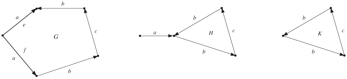
If a finite graph $\Gamma$ is not well-labelled then a process of iterative identifications of each pair $\{e_{1},e_{2}\}$ of distinct edges with the same initial vertex and the same label to a single edge yields a well-labelled graph. Such identifications are called foldings, and the whole process is known as the process of Stallings’ foldings [5, 26, 38, 39].

Thus the graph $\Gamma_{2}$ on Figure 1 is obtained from the graph $\Gamma_{1}$ by folding the edges $e_{1}$ and $e_{2}$ to a single edge labelled by $a$ .

Notice that the graph $\Gamma_{3}$ is obtained from the graph $\Gamma_{2}$ by removing the edge labelled by $a$ whose initial vertex has degree 1. Such an edge is called a hair, and the above procedure is used to be called “cutting hairs”.

The label of a path $p=e_{1}e_{2}\cdots e_{n}$ in $\Gamma$ , where $e_{i}\in E(\Gamma)$ , is the word

lab(p)\equiv lab(e_{1})\cdots lab(e_{n})\in(X^{\pm})^{*}.

Notice that the label of the empty path is the empty word. As usual, we identify the word $lab(p)$ with the corresponding element in $G=gp\langle X|R\rangle$ . We say that $p$ is a normal path (or $p$ is a path in normal form) if $lab(p)$ is a normal word.

If $\Gamma$ is a well-labelled graph then a path $p$ in $\Gamma$ is freely reduced if and only if $lab(p)$ is a freely reduced word. Otherwise $p$ can be converted into a freely reduced path $p^{\prime}$ by iterative removals of the subpaths $e\overline{e}$ (backtrackings) ([38, 26]). Thus

\iota(p^{\prime})=\iota(p),\ \tau(p^{\prime})=\tau(p)\ \;{\rm and}\ \;lab(p)=_{FG(X)}lab(p^{\prime}),

where $FG(X)$ is a free group with a free basis $X$ . We say that $p^{\prime}$ is obtained from $p$ by free reductions.

If $v_{1},v_{2}\in V(\Gamma)$ and $p$ is a path in $\Gamma$ such that

\iota(p)=v_{1},\ \tau(p)=v_{2}\ {\rm and}\ lab(p)\equiv u,

then, following the automata theoretic notation, we simply write $v_{1}\cdot u=v_{2}$ to summarize this situation, and say that the word $u$ is readable at $v_{1}$ in $\Gamma$ .

A pair $(\Gamma,v_{0})$ consisting of the graph $\Gamma$ and the basepoint $v_{0}$ (a distinguished vertex of the graph $\Gamma$ ) is called a pointed graph.

Following the notation of Gitik ([15]) we denote the set of all closed paths in $\Gamma$ starting at $v_{0}$ by $Loop(\Gamma,v_{0})$ , and the image of $lab(Loop(\Gamma,v_{0}))$ in $G=gp\langle X|R\rangle$ by $Lab(\Gamma,v_{0})$ . More precisely,

Loop(\Gamma,v_{0})=\{p\;|\;p{\rm\ is\ a\ path\ in\ \Gamma\ with}\ \iota(p)=\tau(p)=v_{0}\},

Lab(\Gamma,v_{0})=\{g\in G\;|\;\exists p\in Loop(\Gamma,v_{0})\;:\;lab(p)=_{G}g\}.

It is easy to see that $Lab(\Gamma,v_{0})$ is a subgroup of $G$ ([15]). Moreover, $Lab(\Gamma,v)=gLab(\Gamma,u)g^{-1}$ , where $g=_{G}lab(p)$ , and $p$ is a path in $\Gamma$ from $v$ to $u$ ([26]). If $V(\Gamma)=\{v_{0}\}$ and $E(\Gamma)=\emptyset$ then we assume that $H=\{1\}$ .

We say that $H=Lab(\Gamma,v_{0})$ is the subgroup of $G$ determined by the graph $(\Gamma,v_{0})$ . Thus any pointed graph labelled by $X^{\pm}$ , where $X$ is a generating set of a group $G$ , determines a subgroup of $G$ . This argues the use of the name subgroup graphs for such graphs.

Morphisms of Labelled Graphs

Let $\Gamma$ and $\Delta$ be graphs labelled with $X^{\pm}$ . The map $\pi:\Gamma\rightarrow\Delta$ is called a morphism of labelled graphs, if $\pi$ takes vertices to vertices, edges to edges, preserves labels of direct edges and has the property that

\iota(\pi(e))=\pi(\iota(e))\ {\rm and}\ \tau(\pi(e))=\pi(\tau(e)),\ \forall e\in E(\Gamma).

An injective morphism of labelled graphs is called an embedding. If $\pi$ is an embedding then we say that the graph $\Gamma$ embeds in the graph $\Delta$ .

A morphism of pointed labelled graphs $\pi:(\Gamma_{1},v_{1})\rightarrow(\Gamma_{2},v_{2})$ is a morphism of underlying labelled graphs $\pi:\Gamma_{1}\rightarrow\Gamma_{2}$ which preserves the basepoint $\pi(v_{1})=v_{2}$ . If $\Gamma_{2}$ is well-labelled then there exists at most one such morphism ([26]).

Remark 3.1 ([26]).

If two pointed well-labelled (with $X^{\pm}$ ) graphs $(\Gamma_{1},v_{1})$ and $(\Gamma_{2},v_{2})$ are isomorphic, then there exists a unique isomorphism $\pi:(\Gamma_{1},v_{1})\rightarrow(\Gamma_{2},v_{2})$ . Therefore $(\Gamma_{1},v_{1})$ and $(\Gamma_{2},v_{2})$ can be identified via $\pi$ . In this case we sometimes write $(\Gamma_{1},v_{1})=(\Gamma_{2},v_{2})$ . $\diamond$

The notation $\Gamma_{1}=\Gamma_{2}$ means that there exists an isomorphism between these two graphs. More precisely, one can find $v_{i}\in V(\Gamma_{i})$ ( $i\in\{1,2\}$ ) such that $(\Gamma_{1},v_{1})=(\Gamma_{2},v_{2})$ in the sense of Remark 3.1.

4. Subgroup Graphs

The current section is devoted to the discussion on subgroup graphs constructed by the generalized Stallings’ folding algorithm. The main results of [40] concerning these graphs (more precisely, Theorem 7.1, Lemma 8.6, Lemma 8.7, Theorem 8.9 and Corollary 8.11 in [40]), which are essential for the current paper, are summarized in Theorem 4.1 below. All the missing notations are explained along the rest of the present section.

Theorem 4.1.

Let $H=\langle h_{1},\cdots,h_{k}\rangle$ be a finitely generated subgroup of an amalgam of finite groups $G=G_{1}\ast_{A}G_{2}$ .

Then there is an algorithm (the generalized Stallings’ folding algorithm) which constructs a finite labelled graph $(\Gamma(H),v_{0})$ with the following properties:

(1)

${Lab(\Gamma(H),v_{0})}={H}.$
(2)

Up to isomorphism, $(\Gamma(H),v_{0})$ is a unique reduced precover of $G$ determining $H$ .
(3)

A normal word $g\in G$ is in $H$ if and only if it labels a closed path in $\Gamma(H)$ starting at $v_{0}$ , that is $v_{0}\cdot g=v_{0}$ .
(4)

Let $m$ be the sum of the lengths of words $h_{1},\ldots h_{n}$ . Then the algorithm computes $(\Gamma(H),v_{0})$ in time $O(m^{2})$ . Moreover, $|V(\Gamma(H))|$ and $|E(\Gamma(H))|$ are proportional to $m$ .

Corollary 4.2.

Theorem 4.1 (3) provides a solution of the membership problem for finitely generated subgroups of amalgams of finite groups.

Throughout the present paper the notation $(\Gamma(H),v_{0})$ is used for the finite labelled graph constructed by the generalized Stallings’ folding algorithm for a finitely generated subgroup $H$ of an amalgam of finite groups $G=G_{1}\ast_{A}G_{2}$ .

Definition of Precovers:

The notion of precovers was defined by Gitik in [15] for subgroup graphs of amalgams. Below we present its definition and list some basic properties. In doing so, we rely on the notation and results obtained in [15].

In [40] some special cases of precovers, reduced precovers, were considered. However the properties of reduced precovers are irrelevant for the results presented in the current paper. Hence we skip the discussion on them, which can be found in [40].

Let $\Gamma$ be a graph labelled with $X^{\pm}$ , where $X=X_{1}\cup X_{2}$ is the generating set of $G=G_{1}\ast_{A}G_{2}$ given by (1.a)-(1.c). We view $\Gamma$ as a two colored graph: one color for each one of the generating sets $X_{1}$ and $X_{2}$ of the factors $G_{1}$ and $G_{2}$ , respectively.

The vertex $v\in V(\Gamma)$ is called $X_{i}$ -monochromatic if all the edges of $\Gamma$ incident with $v$ are labelled with $X_{i}^{\pm}$ , for some $i\in\{1,2\}$ . We denote the set of $X_{i}$ -monochromatic vertices of $\Gamma$ by $VM_{i}(\Gamma)$ and put $VM(\Gamma)=VM_{1}(\Gamma)\cup VM_{2}(\Gamma)$ .

We say that a vertex $v\in V(\Gamma)$ is bichromatic if there exist edges $e_{1}$ and $e_{2}$ in $\Gamma$ with

\iota(e_{1})=\iota(e_{2})=v\ {\rm and}\ lab(e_{i})\in X_{i}^{\pm},\ i\in\{1,2\}.

The set of bichromatic vertices of $\Gamma$ is denoted by $VB(\Gamma)$ .

A subgraph of $\Gamma$ is called monochromatic if it is labelled only with $X_{1}^{\pm}$ or only with $X_{2}^{\pm}$ . An $X_{i}$ -monochromatic component of $\Gamma$ ( $i\in\{1,2\}$ ) is a maximal connected subgraph of $\Gamma$ labelled with $X_{i}^{\pm}$ , which contains at least one edge. Thus monochromatic components of $\Gamma$ are graphs determining subgroups of the factors, $G_{1}$ or $G_{2}$ .

We say that a graph $\Gamma$ is $G$ -based if any path $p\subseteq\Gamma$ with $lab(p)=_{G}1$ is closed. Thus if $\Gamma$ is $G$ -based then, obviously, it is well-labelled with $X^{\pm}$ .

Definition 4.3 (Definition of Precover).

A $G$ -based graph $\Gamma$ is a precover of $G$ if each $X_{i}$ -monochromatic component of $\Gamma$ is a cover of $G_{i}$ ( $i\in\{1,2\}$ ).

Following the terminology of Gitik ([15]), we use the term “covers of $G$ ” for relative (coset) Cayley graphs of $G$ and denote by $Cayley(G,S)$ the coset Cayley graph of $G$ relative to the subgroup $S$ of $G$ .³³ 3 Whenever the notation $Cayley(G,S)$ is used, it always means that $S$ is a subgroup of the group $G$ and the presentation of $G$ is fixed and clear from the context. If $S=\{1\}$ , then $Cayley(G,S)$ is the Cayley graph of $G$ and the notation $Cayley(G)$ is used.

Note that the use of the term “covers” is adjusted by the well known fact that a geometric realization of a coset Cayley graph of $G$ relative to some $S\leq G$ is a 1-skeleton of a topological cover corresponding to $S$ of the standard 2-complex representing the group $G$ (see [55], pp.162-163).

Convention 4.4.

By the above definition, a precover doesn’t have to be a connected graph. However along this paper we restrict our attention only to connected precovers. Thus any time this term is used, we always mean that the corresponding graph is connected unless it is stated otherwise.

We follow the convention that a graph $\Gamma$ with $V(\Gamma)=\{v\}$ and $E(\Gamma)=\emptyset$ determining the trivial subgroup (that is $Lab(\Gamma,v)=\{1\}$ ) is a (an empty) precover of $G$ . $\diamond$

Example 4.5.

Let $G=gp\langle x,y|x^{4},y^{6},x^{2}=y^{3}\rangle=\mathbb{Z}_{4}\ast_{\mathbb{Z}_{2}}\mathbb{Z}_{6}$ .

Recall that $G$ is isomorphic to $SL(2,\mathbb{Z})$ under the homomorphism

x\mapsto\left(\begin{array}[]{cc}0&1\\ -1&0\end{array}\right),\ y\mapsto\left(\begin{array}[]{cc}0&-1\\ 1&1\end{array}\right).

The graphs $\Gamma_{1}$ and $\Gamma_{3}$ on Figure 2 are examples of precovers of $G$ with one monochromatic component and two monochromatic components, respectively.

Though the $\{x\}$ -monochromatic component of the graph $\Gamma_{2}$ is a cover of $\mathbb{Z}_{4}$ and the $\{y\}$ -monochromatic component is a cover of $\mathbb{Z}_{6}$ , $\Gamma_{2}$ is not a precover of $G$ , because it is not a $G$ -based graph. Indeed, $v\cdot(x^{2}y^{-3})=u$ , while $x^{2}y^{-3}=_{G}1$ .

The graph $\Gamma_{4}$ is not a precover of $G$ because its $\{x\}$ -monochromatic components are not covers of $\mathbb{Z}_{4}$ . $\diamond$

A graph $\Gamma$ is $x$ -saturated at $v\in V(\Gamma)$ , if there exists $e\in E(\Gamma)$ with $\iota(e)=v$ and $lab(e)=x$ ( $x\in X$ ). $\Gamma$ is $X^{\pm}$ -saturated if it is $x$ -saturated for each $x\in X^{\pm}$ at each $v\in V(\Gamma)$ .

Lemma 4.6 (Lemma 1.5 in [15]).

Let $G=gp\langle X|R\rangle$ be a group and let $(\Gamma,v_{0})$ be a graph well-labelled with $X^{\pm}$ . Denote $Lab(\Gamma,v_{0})=S$ . Then

•

$\Gamma$ is $G$ -based if and only if it can be embedded in $(Cayley(G,S),S~\cdot~1)$ ,
•

$\Gamma$ is $G$ -based and $X^{\pm}$ -saturated if and only if it is isomorphic to $(Cayley(G,S),S\cdot~1)$ . ⁴⁴ 4 We write $S\cdot 1$ instead of the usual $S1=S$ to distinguish this vertex of $Cayley(G,S)$ as the basepoint of the graph.

Corollary 4.7.

If $\Gamma$ is a precover of $G$ with $Lab(\Gamma,v_{0})=H\leq G$ then $\Gamma$ is a subgraph of $Cayley(G,H)$ .

Thus a precover of $G$ can be viewed as a part of the corresponding cover of $G$ , which explains the use of the term “precovers”.

Remark 4.8 ([40]).

Let $\phi:\Gamma\rightarrow\Delta$ be a morphism of labelled graphs. If $\Gamma$ is a precover of $G$ , then $\phi(\Gamma)$ is a precover of $G$ as well. $\diamond$

Precovers are Compatible:

A graph $\Gamma$ is called compatible at a bichromatic vertex $v$ if for any monochromatic path $p$ in $\Gamma$ such that $\iota(p)=v$ and $lab(p)\in A$ there exists a monochromatic path $t$ of a different color in $\Gamma$ such that $\iota(t)=v$ , $\tau(t)=\tau(p)$ and $lab(t)=_{G}lab(p)$ . We say that $\Gamma$ is compatible if it is compatible at all bichromatic vertices.

Example 4.9.

The graphs $\Gamma_{1}$ and $\Gamma_{3}$ on Figure 2 are compatible. The graph $\Gamma_{2}$ does not possess this property because $w\cdot x^{2}=v$ , while $w\cdot y^{3}=u$ . $\Gamma_{4}$ is not compatible as well. $\diamond$

Lemma 4.10 (Lemma 2.12 in [15]).

If $\Gamma$ is a compatible graph, then for any path $p$ in $\Gamma$ there exists a path $t$ in normal form such that $\iota(t)=\iota(p),\ \tau(t)=\tau(p)\ {\rm and}\ lab(t)=_{G}lab(p).$

Remark 4.11 (Remark 2.11 in [15]).

Precovers are compatible. $\diamond$

The following can be taken as another definition of precovers.

Lemma 4.12 (Corollary2.13 in [15]).

Let $\Gamma$ be a compatible graph. If all $X_{i}$ -components of $\Gamma$ are $G_{i}$ -based, $i\in\{1,2\}$ , then $\Gamma$ is $G$ -based. In particular, if each $X_{i}$ -component of $\Gamma$ is a cover of $G_{i}$ , $i\in\{1,2\}$ , and $\Gamma$ is compatible, then $\Gamma$ is a precover of $G$ .

Complexity Issues:

As were noted in [40], the complexity of the generalized Stallings’ algorithm is quadratic in the size of the input, when we assume that all the information concerning the finite groups $G_{1}$ , $G_{2}$ , $A$ and the amalgam $G=G_{1}\ast_{A}G_{2}$ given via $(1.a)$ , $(1.b)$ and $(1.c)$ (see Section 3) is not a part of the input. We also assume that the Cayley graphs and all the relative Cayley graphs of the free factors are given for “free” as well.

Otherwise, if the group presentations of the free factors $G_{1}$ and $G_{2}$ , as well as the monomorphisms between the amalgamated subgroup $A$ and the free factors are a part of the input (the uniform version of the algorithm) then we have to build the groups $G_{1}$ and $G_{2}$ , that is to construct their Cayley graphs and relative Cayley graphs.

Since we assume that the groups $G_{1}$ and $G_{2}$ are finite, the Todd-Coxeter algorithm and the Knuth Bendix algorithm are suitable [36, 53, 55] for these purposes. Then the complexity of the construction depends on the group presentation of $G_{1}$ and $G_{2}$ we have: it could be even exponential in the size of the presentation [10]. Therefore the generalized Stallings algorithm, presented in [40], with these additional constructions could take time exponential in the size of the input.

Thus each uniform algorithmic problem for $H$ whose solution involves the construction of the subgroup graph $\Gamma(H)$ may have an exponential complexity in the size of the input.

The primary goal of the complexity analysis introduced along the current paper is to estimate our graph theoretical methods. To this end, we assume that all the algorithms along the present paper have the following “given data”.

GIVEN:: : Finite groups $G_{1}$ , $G_{2}$ , $A$ and the amalgam $G=G_{1}\ast_{A}G_{2}$ given via $(1.a)$ , $(1.b)$ and $(1.c)$ .
We assume that the Cayley graphs and all the relative Cayley graphs of the free factors are given.

5. Computing Subgroup Presentations

Given a presentation of a group $G$ , and a suitable information about a subgroup $H$ of $G$ , the Reidemeister-Schreier method (see 2.2.3 in [37]) enables one to compute a presentation for $H$ .

It’s a well known fact (see, for instance, [37], p.90) that if $[G:H]<\infty$ then $H$ is finitely generated when $G$ is finitely generated, and $H$ is finitely presented when $G$ is finitely presented. Such a finite presentation of $H$ can be effectively calculated by an application of the Reidemeister-Schreier method.

However a subgroup can be finitely presented even if its index is infinite. For instance, if the group under the consideration is coherent, then all its finitely generated subgroups are finitely presented. Recently, coherence of some classes of groups has been investigated in [43, 47].

Below we introduce a restricted version of the Reidemeister-Schreier method which allows to compute a finite presentation for a finitely generated subgroup $H$ of an amalgam of finite groups $G=G_{1}\ast_{A}G_{2}$ given by (1.a)-(1.c). This immediately implies the coherence of amalgams of finite groups.

The suitable information about the subgroup which is needed for an application of the method can be read off from its subgroup graph $\Gamma(H)$ constructed by the generalized Stallings’ algorithm.

Let $(\Gamma,v_{0})$ be a finite precover of $G$ . Let $H=Lab(\Gamma,v_{0})$ .

Recall that $H=Lab(\Gamma,v_{0})$ is the image of $lab(Loop(\Gamma,v_{0}))\subseteq X^{*}$ in $G$ under the natural morphism $\varphi:X^{*}{\rightarrow}G$ . Note that $\varphi=\varphi_{2}\circ\varphi_{1}$ , where

\varphi_{1}:X^{*}\rightarrow FG(X)\ {\rm and}\ \varphi_{2}:FG(X)\rightarrow G.

Let $\widetilde{H}=\varphi_{1}\left(lab(Loop(\Gamma,v_{0})\right)$ . Thus $H=\varphi_{2}(\widetilde{H})$ . Moreover,

H=\widetilde{H}/N=\widetilde{H}/\left(\widetilde{H}\cap N\right),

where $N$ is the normal closure of $R$ in $FG(X)$ (see [36, 37]). We put $F=FG(X)$ .

Let $T$ be a fixed spanning tree of $\Gamma$ . For all $v\in V(\Gamma)$ , we consider $t_{v}$ to be the unique freely reduced path in $T$ from the basepoint $v_{0}$ to the vertex $v$ .

For each $e\in E(\Gamma)$ we consider $t(e)=t_{\iota(e)}e\overline{t_{\tau(e)}}$ . Thus if $e\in E(T)$ then $t(e)$ can be freely reduced to an empty path, that is $lab(t(e))=_{F}1$ .

Let $E^{+}$ be the set of positively oriented edges of $\Gamma$ . Let

(1)

X_{H}=\{lab(t(e))\;|\;e\in E^{+}\setminus E(T)\},

Q_{v}=\{q\subseteq\Gamma\;|\;\iota(q)=\tau(q)=v,\;lab(q)\equiv r\in R\},

(2)

R_{H}=\left\{lab\left(\phi\left(t_{v}q\overline{t_{v}}\right)\right)\;|v\in V(\Gamma),\;t_{v}\subseteq T,\;q\in Q_{v},\right\},

where $\phi$ is a function from the set of freely reduced paths in $\Gamma$ into $Loop(\Gamma,v_{0})$ defined as follows.

\phi(p)=t(e_{1})t(e_{2})\cdots t(e_{n}),\ {\rm where}\ p=e_{1}e_{2}\cdots e_{n}\subseteq\Gamma.

Thus the path $\phi(p)$ is closed at $v_{0}$ in $\Gamma$ and

lab(\phi(p))\equiv lab(t(e_{1}))lab(t(e_{2}))\cdots lab(t(e_{n})).

Moreover, if the path $p$ is closed at $v_{0}$ in $\Gamma$ then the path $\phi(p)$ is freely equivalent to $p$ , that is $\phi(p)$ can be transformed to the path $p$ by a series of free reductions. Thus $lab(\phi(p))=_{F}lab(p)$ .

The function $\phi$ induces a partial function $\phi^{\prime}$ from $FG(X)$ into $FG(X_{H})$ such that $\phi^{\prime}(w)=lab(\phi(p))$ , where $p$ is a path in $\Gamma$ with $lab(p)\equiv w$ . Thus another definition of $R_{H}$ takes the following form

(3)

R_{H}=\left\{\phi^{\prime}\left(lab(t_{v}q\overline{t_{v}})\right)\;|\;v\in V(\Gamma),\;t_{v}\subseteq T,\;q\in Q_{v},\right\}.

Remark 5.1.

Note that the system of coset representatives $\{lab(t_{v})\;|\;v\in V(\Gamma)\}$ is a subset of the Schreier transversal of $\widetilde{H}$ in $FG(X)$ ([54]). $\diamond$

Theorem 5.2.

With the above notation, $H=gp\langle X_{H}\;|R_{H}\rangle$ .

Proof.

As is well known ([26, 38, 54]), $\widetilde{H}=FG(X_{H})$ . Therefore $H=\langle X_{H}\rangle$ .

To complete the proof it remains to show that the normal closure $N_{H}$ of $R_{H}$ in $FG(X_{H})=\widetilde{H}$ is equal to $\widetilde{H}\cap N$ .

Let $v\in V(\Gamma)$ such that $Q_{v}\neq\emptyset$ . Let $q\in Q_{v}$ . Therefore $\phi(t_{v}q\overline{t_{v}})$ is freely equivalent to the path $t_{v}q\overline{t_{v}}$ . Thus

lab(\phi(t_{v}q\overline{t_{v}}))=_{F}lab(t_{v}q\overline{t_{v}})\equiv lab(t_{v})lab(q)lab(t_{v})^{-1}\in N.

On the other hand, the path $t_{v}q\overline{t_{v}}$ is closed at $v_{0}$ , hence $lab(t_{v}q\overline{t_{v}})\in\widetilde{H}$ . Thus $lab(\phi(t_{v}q\overline{t_{v}}))\in\widetilde{H}\cap N$ . Therefore $R_{H}\subseteq\widetilde{H}\cap N$ .

For all $y\in\widetilde{H}$ , there exist a closed path $s\in\Gamma$ starting at $v_{0}$ with $lab(s)=_{F}\widetilde{H}$ . By the definition of $R_{H}$ , for all $r\in R_{H}$ there exist a path $t_{v}q\overline{t_{v}}\subseteq\Gamma$ closed at $v_{0}$ such that $lab(t_{v}q\overline{t_{v}})=_{F}r$ . Hence the path $s(t_{v}q\overline{t_{v}})\overline{s}$ is closed at $v_{0}$ in $\Gamma$ . Thus $lab(s(t_{v}q\overline{t_{v}})\overline{s})=_{F}yry^{-1}\in\widetilde{H}$ . Moreover, $lab(s(t_{v}q\overline{t_{v}})\overline{s})\equiv lab(st_{v})lab(q)(lab(st_{v}))^{-1}\in N$ . Therefore $N_{H}\subseteq\widetilde{H}\cap N$ .

Assume now that $w\in\widetilde{H}\cap N$ . Since $w\in\widetilde{H}$ , there exists a freely reduced path $p$ in $\Gamma$ closed at $v_{0}$ with $lab(p)=_{F}w$ ([26, 38]). Let $p=p_{1}\cdots p_{k}$ be its decomposition into maximal monochromatic paths $p_{i}$ with $lab(p_{i})\equiv w_{i}\in G_{l_{i}}$ ( $1\leq i\leq k$ and $l_{i}\in\{1,2\}$ ).

Since $w\in N$ , $w=_{G}1$ . Therefore, by the Normal Form Theorem for free products with amalgamation (IV.2.6 in [36]), there exists $1\leq i\leq k$ such that $w_{i}\in A\cap G_{l_{i}}$ . The proof is by induction on the number $k$ of the maximal monochromatic subpaths of the path $p$ . Without loss of generality, simplifying the notation, we let $l_{i}=1$ .

Assume first that $w_{i}=_{G_{1}}1$ . Since $\Gamma$ is $G$ -based, the subpath $p_{i}$ is closed at $\iota(p_{i})=\tau(p_{i})$ .

Let $v_{j}=\tau(p_{j})$ and let $t_{j}=t_{v_{j}}\subseteq T$ ( $1\leq j\leq k$ ). Thus $v_{i-1}=v_{i}$ and $t_{i-1}=t_{i}$ . Let $t=p_{1}\cdots p_{i-1}$ . See Figure 3 (a).

Hence the path $p$ can be obtained by free reductions from the following path

\left(\>(t\overline{t}_{i-1})(t_{i-1}p_{i}\overline{t_{i-1}})(t_{i-1}\overline{t})\>\right)\left(tp_{i+1}\cdots p_{k}\right).

Thus $lab(t\overline{t}_{i-1})\in\widetilde{H}$ , and the number of the maximal monochromatic subpaths of the path

tp_{i+1}\cdots p_{k}=p_{1}\cdots p_{i-2}(p_{i-1}p_{i+1})p_{i+2}\cdots p_{k}

is $k-2$ . Therefore, by the inductive assumption, $lab(tp_{i+1}\cdots p_{k})\in N_{H}$ . To get the desired conclusion it remains to show that $lab(t_{i-1}p_{i}\overline{t_{i-1}})\in N_{H}$ .

Since $w_{i}=_{G_{1}}1$ , we have $lab(p_{i})\in N_{1}$ , where $N_{1}$ is the normal closure of $R_{1}$ in $F_{1}=FG(X_{1})$ . Therefore $lab(p_{i})=_{F_{1}}(z_{1}s_{1}z_{1}^{-1})\cdots(z_{m}s_{m}z_{m}^{-1})$ , where $z_{j}\in F_{1}$ and $s_{j}\in R_{1}$ ( $1\leq j\leq m$ ).

Let $C_{i}$ be the $X_{1}$ -monochromatic component of $\Gamma$ such that $p_{i}\subseteq C_{i}$ . Since $\Gamma$ is a precover of $G$ , $C$ is $X_{1}^{\pm}$ -saturated. Hence $p_{i}$ is a free reduction of the path $p_{i}^{\prime}\subseteq C$ such that $lab(p_{i}^{\prime})\equiv(z_{1}s_{1}z_{1}^{-1})\cdots(z_{m}s_{m}z_{m}^{-1})$ . Since $\Gamma$ is $G$ -based, the subpaths of $p_{i}^{\prime}$ labelled by $s_{j}$ ( $1\leq j\leq m$ ) are closed. Therefore $p_{i}^{\prime}$ has the following decomposition

p_{i}^{\prime}=(c_{1}q_{1}\overline{c_{1}})\cdots(c_{m}q_{m}\overline{c_{m}}),

where $lab(c_{j})\equiv z_{j}$ and $lab(q_{j})\equiv s_{j}$ ( $1\leq j\leq m$ ). Thus the path $t_{i-1}p_{i}\overline{t_{i-1}}$ can be obtained by free reductions from the path

\left(t_{i-1}(c_{1}q_{1}\overline{c_{1}})\overline{t_{i-1}}\right)\cdots\left(t_{i-1}(c_{m}q_{m}\overline{c_{m}})\overline{t_{i-1}}\right).

For each $1\leq j\leq m$ , the path $t_{i-1}(c_{j}q_{j}\overline{c_{j}})\overline{t_{i-1}}$ is a free reduction of the path

(t_{i-1}c_{1}\overline{t_{\tau(c_{j})}})(t_{\tau(c_{j})}q_{j}\overline{t_{\tau(c_{j})}})(\overline{t_{i-1}c_{j}\overline{t_{\tau(c_{j})}}}).

Since $lab(t_{i-1}c_{j}\overline{t_{\tau(c_{j})}})\in\widetilde{H}$ and $lab(\phi(t_{\tau(c_{j})}q_{j}\overline{t_{\tau(c_{j})}}))\in R_{H}$ we conclude that $lab(t_{i-1}(c_{j}q_{j}\overline{c_{j}})\overline{t_{i-1}})\in N_{H}$ ( $1\leq j\leq m$ ). Therefore $lab(t_{i-1}p_{i}\overline{t_{i-1}})\in N_{H}$ . We are done.

Assume now that $1\neq_{G}w_{i}\in A\cap G_{1}$ .

Since for all $1\leq j\leq k$ the vertices $v_{j}=\tau(p_{j})$ are bichromatic, and because the graph $\Gamma$ is compatible, there exists a $X_{2}$ -monochromatic path $p_{i}^{\prime}$ in $\Gamma$ such that $\iota(p_{i}^{\prime})=\iota(p_{i})$ , $\tau(p_{i}^{\prime})=\tau(p_{i})$ and $lab(p_{i}^{\prime})=_{G}lab(p_{i})$ . See Figure 3 (b). Hence the path $p$ can be obtained by free reductions from the following path

\left(\>(t\overline{t}_{i-1})(t_{i-1}p_{i}\overline{p_{i}^{\prime}}\overline{t_{i-1}})(t_{i-1}\overline{t})\>\right)\left(tp^{\prime}_{i}p_{i+1}\cdots p_{k}\right).

Thus $lab(t\overline{t}_{i-1})\in\widetilde{H}$ , and the number of the maximal monochromatic subpaths of the path

tp^{\prime}_{i}p_{i+1}\cdots p_{k}=p_{1}\cdots p_{i-2}(p_{i-1}p^{\prime}_{i}p_{i+1})p_{i+2}\cdots p_{k}

is $k-2$ . Therefore, by the inductive assumption, $lab(tp^{\prime}_{i}p_{i+1}\cdots p_{k})\in N_{H}$ . To get the desired conclusion it remains to show that $lab(t_{i-1}(p_{i}\overline{p^{\prime}_{i}})\overline{t_{i-1}})\in N_{H}$ .

Let $lab(p_{i})=_{G_{1}}a_{1}\cdots a_{m}$ , where $a_{j}$ are generators of $A\cap G_{1}$ . Let $b_{j}$ be corresponding generators of $A\cap G_{2}$ such that $a_{j}=_{G}b_{j}$ and $a_{j}{b_{j}}^{-1}\in R$ ( $1\leq j\leq m$ ). Note that

(a_{1}\cdots a_{m})(b_{1}\cdots b_{m})^{-1}=_{F}

=_{F}\left(a_{1}{b_{1}}^{-1}\right)\left(b_{1}\left(a_{2}{b_{2}}^{-1}\right)b_{1}^{-1}\right)\cdots\left(b_{1}\cdots b_{m-1}\left(a_{m}b_{m}^{-1}\right)b_{m-1}^{-1}\cdots b_{1}^{-1}\right).

Since monochromatic components of $\Gamma$ are $X_{i}^{\pm}$ -saturated ( $i\in\{1,2\}$ ), and because $\iota(p_{i})\in VB(\Gamma)$ , there exist paths $\gamma_{1}$ and $\delta_{1}$ such that $\iota(\gamma_{1})=\iota(p_{i})=\iota(\delta_{1})$ and $lab(\gamma_{1})\equiv a_{1}$ , $lab(\delta_{1})\equiv b_{1}$ . Since $\Gamma$ is compatible, $\tau(\gamma_{1})=\tau(\delta_{1})\in VB(\Gamma)$ . Thus there exist paths $\gamma_{2}$ and $\delta_{2}$ such that $\iota(\gamma_{2})=\tau(\gamma_{1})=\iota(\delta_{2})$ and $lab(\gamma_{2})\equiv a_{2}$ , $lab(\delta_{2})\equiv b_{2}$ . Since $\Gamma$ is compatible, $\tau(\gamma_{2})=\tau(\delta_{2})\in VB(\Gamma)$ .

Continuing in this manner one can construct such paths $\gamma_{j}$ , $\delta_{j}$ for all $1\leq j\leq m$ . Thus $p_{i}$ and $p^{\prime}_{i}$ are free reductions of the paths $\gamma_{1}\cdots\gamma_{m}$ and $\delta_{1}\cdots\delta_{m}$ , respectively. Hence the path $p_{i}\overline{p_{i}^{\prime}}$ can be obtained by free reductions from the path

\left(\gamma_{1}{\overline{\delta_{1}}}\right)\left(\delta_{1}\left(\gamma_{2}{\overline{\delta_{2}}}\right)\overline{\delta_{1}}\right)\cdots\left(\delta_{1}\cdots\delta_{m-1}\left(\gamma_{m}\overline{\delta_{m}}\right)\overline{\delta_{m-1}}\cdots\overline{\delta_{1}}\right).

Therefore the path $t_{i-1}(p_{i}\overline{p_{i}^{\prime}})\overline{t}_{i-1}$ is a free reduction of

\left(t_{i-1}(\gamma_{1}{\overline{\delta_{1}}})\overline{t}_{i-1}\right)\cdots\left(t_{i-1}(\delta_{1}\cdots\delta_{m-1}\left(\gamma_{m}\overline{\delta_{m}}\right)\overline{\delta_{m-1}}\cdots\overline{\delta_{1}})\overline{t}_{i-1}\right).

For each $1\leq j\leq m-1$ , the path $t_{i-1}(\delta_{1}\cdots\delta_{j-1}\left(\gamma_{j}\overline{\delta_{j}}\right)\overline{\delta_{j-1}}\cdots\overline{\delta_{1}})\overline{t}_{i-1}$ is a free reduction of the path

\left(t_{i-1}\delta_{1}\cdots\delta_{j-1}\overline{t_{\iota(\gamma_{j})}}\right)\left(t_{\iota(\gamma_{j})}(\gamma_{j}{\overline{\delta_{j}}})\overline{t_{\iota(\gamma_{j})}}\right)\left(t_{\iota(\gamma_{j})}\overline{\delta_{j-1}}\cdots\overline{\delta_{1}}\overline{t_{i-1}}\right).

Since $lab\left(\phi\left(t_{\iota(\gamma_{j})}(\gamma_{j}\overline{\delta_{j}})\overline{t_{\iota(\gamma_{j})}}\right)\right)\in R_{H}$ and $lab(t_{i-1}\delta_{1}\cdots\delta_{j-1}\overline{t_{\iota(\gamma_{j})}})\in\widetilde{H}$ , we conclude that for each $1\leq j\leq m-1$

lab(t_{i-1}(\delta_{1}\cdots\delta_{j-1}\left(\gamma_{j}\overline{\delta_{j}}\right)\overline{\delta_{j-1}}\cdots\overline{\delta_{1}})\overline{t}_{i-1})\in N_{H}.

Therefore $lab(t_{i-1}(p_{i}\overline{p_{i}^{\prime}})\overline{t_{i-1}})\in N_{H}$ . We are done.

∎

Corollary 5.3.

Let $(\Gamma,v_{0})$ be a finite precover of $G$ . Then there exists an algorithm which computes a subgroup of $G$ determined by $(\Gamma,v_{0})$ , that is computes a finite group presentation of $H=Lab(\Gamma,v_{0})$ .

Proof.

We compute the sets $X_{H}$ and $R_{H}$ according to their definitions. These sets are finite, because the graph $\Gamma$ is finite. By Theorem 5.2, $H=gp\langle X_{H}\;|\;R_{H}\rangle$ .

∎

Corollary 5.4.

Let $h_{1},\ldots h_{n}\in G$ . Then there exists an algorithm which computes a finite group presentation of the subgroup $H=\langle h_{1},\ldots,h_{n}\rangle$ in $G$ (not necessary with respect to $\{h_{1},\cdots,h_{n}\}$ ) .

Proof.

We first construct the graph $(\Gamma(H),v_{0})$ , using the generalized Stallings’ folding algorithm. By Theorem 4.1 (2), this graph is a finite precover of $G$ . Now we proceed according to Corollary 5.3.

∎

Corollary 5.5.

Amalgams of finite groups are coherent.

Remark 5.6.

As is well known, the Reidemeister-Schreier method yields a presentation of a subgroup $H$ which is usually not in a useful form. Namely, some of the generators are redundant and can be eliminated, while some of the relators can be simplified. In order to improve (to simplify) this presentation, one can apply the Tietze transformation. An efficient version of such a simplification procedure was developed in [22, 23]. $\diamond$

Example 5.7.

Let $G=gp\langle x,y|x^{4},y^{6},x^{2}(y^{3})^{-1}\rangle=\mathbb{Z}_{4}\ast_{\mathbb{Z}_{2}}\mathbb{Z}_{6}$ .

Recall that $G$ is isomorphic to $SL(2,\mathbb{Z})$ under the homomorphism

x\mapsto\left(\begin{array}[]{cc}0&1\\ -1&0\end{array}\right),\ y\mapsto\left(\begin{array}[]{cc}0&-1\\ 1&1\end{array}\right).

Let $H=\langle xyx^{-1},yxy^{-1}\rangle$ be a subgroup of $G$ . The subgroup graph $\Gamma(H)$ constructed by the generalized Stallings’ folding algorithm is presented on Figure 4.

We apply to $\Gamma(H)$ the algorithm described along with the proof of Corollary 5.4.

We first compute $X_{H}$ according to (1):

h_{1}=xyx^{-1},\ h_{2}=x^{2},\ h_{3}=yxy^{-1},\ h_{4}=y^{3}.

The computation of $R_{H}$ according to (3) consists of the following steps.

\phi^{\prime}(x^{4})=(h_{2})^{2},\ \phi^{\prime}(y^{6})=(h_{4})^{2},\ \phi^{\prime}(x^{2}(y^{3})^{-1})=h_{2}(h_{4})^{-1}.

\phi^{\prime}(x(x^{4})x^{-1})=(h_{2})^{2},\ \phi^{\prime}(x(y^{6})x^{-1})=(h_{1})^{6},\ \phi^{\prime}(x(x^{2}(y^{3})^{-1})x^{-1})=h_{2}(h_{1})^{-3}.

\phi^{\prime}(y(x^{4})y^{-1})=(h_{3})^{4},\ \phi^{\prime}(y(y^{6})y^{-1})=(h_{4})^{2},\ \phi^{\prime}(y(x^{2}(y^{3})^{-1})y^{-1})=h_{3}^{2}(h_{4})^{-1}.

Therefore $H=gp\langle h_{1},h_{3}\;|\;h_{1}^{6},h_{3}^{4},h_{1}^{3}=h_{3}^{2}\rangle$ .

$\diamond$

Complexity.

Let $m$ be the sum of the lengths of the words $h_{1},\ldots h_{n}$ . By Theorem 4.1 $(4)$ , the generalized Stallings’ algorithm computes $(\Gamma(H),v_{0})$ in time $O(m^{2})$ .

The construction of $X_{H}$ , which is a free basis of $\widetilde{H}=\varphi_{1}\left(lab(Loop(\Gamma(H),v_{0})\right)$ , takes $O(|E(\Gamma(H))|^{2})$ , by [5]. Since, by Theorem 4.1 $(4)$ , $|E(\Gamma(H))|$ is proportional to $m$ , the computation of $X_{H}$ takes $O(m^{2})$ .

To construct the set $Q_{H}$ we try to read each one of the defining relators of $G$ at each one of the vertices of the graph $\Gamma(H)$ . It takes at most

|R|\cdot|V(\Gamma(H)|\cdot\left(\sum_{v\in V(\Gamma(H))}deg(v)\right).

Since $\sum_{v\in V(\Gamma(H))}deg(v)=2|E(\Gamma(H)|$ and because, by our assumption, the presentation of $G$ is given and it is not a part of the input, the computation of the set $Q_{H}$ takes $O(|V(\Gamma(H)|\cdot|E(\Gamma(H)|)$ . Since, by Theorem 4.1 (4), $|V(\Gamma(H)|=O(m)$ , it takes $O(m^{2})$ .

The rewriting process which yield the set of relators $R_{H}$ takes at most $|V(\Gamma(H)|\cdot\left(\sum_{r\in R}|r|\right)$ which is $O(|V(\Gamma(H)|)$ .

Thus the complexity of the restricted Reidemeister-Schreier process given by Corollary 5.4 is $O(m^{2})$ .

6. The Freeness Problem

A freeness of subgroups is one of the fundamental questions of combinatorial and geometric group theory. The classical results in this issue include the Nielsen-Schreier subgroup theorem for free groups, the corollary of Kurosh subgroup theorem and the Freiheitssatz of Magnus.

Namely, subgroups of free groups are free (I.3.8, [36]). A subgroup of a free product which has a trivial intersection with all conjugates of the factors is free ([36], p.120). A subgroup $H$ of an one-relator group $G=gp\langle X\;|\;r=1\rangle$ , where $r$ is cyclically freely reduced, is free if $H$ is generated by a subset of $X$ which omits a generator occurring in $r$ (II.5.1, [36]).

Results concerning amalgamated free products follow from the Neumann’s subgroup theorem.

Theorem 6.1 (H.Neumann, IV.6.6 [36]).

Let $G=G_{1}\ast_{A}G_{2}$ be a non-trivial free product with amalgamation. Let $H$ be a finitely generated subgroup of $G$ such that all conjugates of $H$ intersect $A$ trivially.

Then $H=F\ast(\ast_{j}\;g_{j}H_{j}g_{j}^{-1})$ , where $F$ is a free group and each $H_{j}$ is the intersection of a subgroup of $H$ with a conjugate of a factor of $G$ .

Corollary 6.2 (IV.6.7 [36]).

Let $G=G_{1}\ast_{A}G_{2}$ be a non-trivial free product with amalgamation. If $H$ is a finitely generated subgroup of $G$ which has trivial intersection with all conjugates of the factors, $G_{1}$ and $G_{2}$ , of $G$ , then $H$ is free.

It turns out (Lemma 6.3) that the triviality of the intersections between $H$ and conjugates of the factors, $G_{1}$ and $G_{2}$ , of $G$ can be detected from the subgroup graph $\Gamma(H)$ constructed by the generalized Stallings’ folding algorithm, when $G=G_{1}\ast_{A}G_{2}$ is an amalgam of finite groups. Therefore, by Corollary 6.2, the freeness of $H$ is decidable via its subgroup graph.

We consider the freeness problem to be one which asks to verify if a subgroup of a given group $G$ is free. Clearly, the freeness problem is solvable in amalgams of finite groups.

Below we introduce a polynomial time algorithm (Corollary 6.7) that employs subgroup graphs constructed by the generalized Stallings’ algorithm to solve the freeness problem. A complexity analysis of the algorithm is given at the end of the section.

Lemma 6.3.

Let $H$ be a finitely generated subgroup of an amalgam of finite groups $G=G_{1}\ast_{A}G_{2}$ .

Then $H$ has a trivial intersection with all conjugates of the factors of $G$ if and only if each $X_{i}$ -monochromatic component $C$ of $\Gamma(H)$ is isomorphic to $Cayley(G_{i})$ , for all $i\in\{1,2\}$ . Equivalently, by Lemma 4.6, if and only if $Lab(C,v)=\{1\}$ for each $X_{i}$ -monochromatic component $C$ of $\Gamma(H)$ ( $v\in V(C)$ ).

Proof.

Assume first that there exists a $X_{i}$ -monochromatic component $C$ of $\Gamma(H)$ ( $i\in\{1,2\}$ ) which is not isomorphic to $Cayley(G_{i})$ . Thus, by Lemma 4.6, $(C,\vartheta)$ is not isomorphic to $Cayley(G_{i},S,S\cdot 1)$ , where is $\vartheta\in V(C)$ and $\{1\}\neq S\leq G_{i}$ .

Let $1\neq_{G}w\in S$ . Then there exists a path $q$ in $C$ closed at $\vartheta$ such that $lab(q)\equiv w$ . Let $p$ be an approach path in $\Gamma(H)$ from $\iota(p)=v_{0}$ to $\tau(p)=\vartheta$ . Let $u\equiv lab(p)$ .

The path $pq\overline{p}$ is closed at $v_{0}$ in $\Gamma(H)$ . Hence $lab(pq\overline{p})\in H$ . Therefore

lab(pq\overline{p})=_{G}uwu^{-1}\in H\cap uLab(C,\vartheta)u^{-1}=H\cap uSu^{-1}.

Since $w\neq_{G}1$ , we have $uwu^{-1}\neq_{G}1$ and hence $H\cap uSu^{-1}\neq\{1\}$ .

Assume now that there exists $\{1\}\neq S\leq G_{i}$ ( $i\in\{1,2\}$ ) such that $H\cap uSu^{-1}\neq\{1\}$ , where $u\in G$ . Let $1\neq_{G}h\in H\cap uSu^{-1}$ . Thus $h=_{G}ugu^{-1}$ , where $1\neq_{G}g\in S$ . Without loss of generality we can assume that the words $u$ and $g$ are normal.

If the word $ugu^{-1}$ is in normal form, then there exist a path $p$ in $\Gamma(H)$ closed at $v_{0}$ such that $lab(p)\equiv ugu^{-1}$ . Thus there is a decomposition $p=p_{1}p_{2}\overline{p_{1}}$ (because $\Gamma(H)$ is $G$ -based, so it is a well-labelled graph), where $lab(p_{1})\equiv u$ and $lab(p_{2})\equiv g$ . Let $C$ be a $X_{i}$ -monochromatic component of $\Gamma(H)$ such that $p_{2}\subseteq C$ and let $v=\tau(p_{1})$ . Hence $g\equiv lab(p_{2})\in Lab(C,v)\leq G_{i}$ . Thus $Lab(C,v)\neq\{1\}$ . Equivalently, by Lemma 4.6, $C$ is not isomorphic to $Cayley(G_{i})$ .

Assume now that the word $ugu^{-1}$ is not in normal form. Let $(u_{1},\ldots,u_{k})$ be a normal decomposition of $u$ . Since $g\in G_{i}$ , its normal decomposition is $(g)$ . Hence the normal decomposition of $ugu^{-1}$ has the form

(u_{1},\ldots,u_{j-1},w,u_{j-1}^{-1},\ldots,u_{1}^{-1}),

where $w=_{G}u_{j}\ldots u_{k}gu_{k}^{-1}\ldots u_{j}^{-1}\in G_{l}\setminus A$ and $u_{j-1}\in G_{m}\setminus A$ ( $1\leq l\neq m\leq 2$ ).

Let $u^{\prime}\equiv u_{1}\ldots u_{j-1}$ . Then $h=_{G}u^{\prime}w(u^{\prime})^{-1}$ , while the word $u^{\prime}w(u^{\prime})^{-1}$ is in normal form and $w\in G_{l}$ , $l\in\{1,2\}$ . Hence, by arguments similar to those used in the previous case, we are done.

∎

Theorem 6.4.

Let $H$ be a finitely generated subgroup of an amalgam of finite groups $G=G_{1}\ast_{A}G_{2}$ .

Then $H$ is free if and only if each $X_{i}$ -monochromatic component of $\Gamma(H)$ is isomorphic to $Cayley(G_{i})$ , for all $i\in\{1,2\}$ .

Proof.

The statement follows immediately from Corollary 6.2 and Lemma 6.3. ∎

Combining Lemma 6.3 with the Torsion Theorem for amalgamated free products we get Corollary 6.6.

Theorem 6.5 (Torsion Theorem, IV.2.7, [36]).

Every element of finite order in $G=G_{1}\ast_{A}G_{2}$ is a conjugate of an element of finite order in $G_{1}$ or $G_{2}$ .

Corollary 6.6.

Let $H$ be a finitely generated subgroup of an amalgam of finite groups $G=G_{1}\ast_{A}G_{2}$ .

Then $H$ is torsion free if and only if each $X_{i}$ -monochromatic component of $\Gamma(H)$ is isomorphic to $Cayley(G_{i})$ , for all $i\in\{1,2\}$ .

Corollary 6.7.

Let $h_{1},\ldots,h_{k}\in G.$ Then there exists an algorithm which decides whether or not the subgroup $H=\langle h_{1},\ldots,h_{k}\rangle$ is a free subgroup of $G$ .

Proof.

We first construct the graph $\Gamma(H)$ , using the generalized Stallings’ folding algorithm.

Now, for each $X_{i}$ -monochromatic component $C$ of $\Gamma(H)$ we verify if $C$ is isomorphic to $Cayley(G_{i})$ ( $i\in\{1,2\}$ ). It can be easily done by checking the number of vertices of $C$ : $|V(C)|=|G_{i}|$ if and only if $C$ is isomorphic to $Cayley(G_{i})$ .

By Theorem 6.4, $H$ is free if and only if each monochromatic component of $\Gamma(H)$ is isomorphic to the Cayley graph of an appropriate factor of $G$ .

∎

Remark 6.8.

If $H$ is free then its free basis can be computed using the restricted Reidemeister-Schreier procedure (Corollary 5.4) followed by a simplification process based on Tietze transformation. For an effective version of a simplification procedure when redundant generators are eliminated consequently using a substring search technique see [22, 23]. $\diamond$

Example 6.9.

Let $G=gp\langle x,y|x^{4},y^{6},x^{2}=y^{3}\rangle=\mathbb{Z}_{4}\ast_{\mathbb{Z}_{2}}\mathbb{Z}_{6}$ .

Let $H_{1}$ and $H_{2}$ be finitely generated subgroups of $G$ such that

H_{1}=\langle xy\rangle\ {\rm and}\ H_{2}=\langle xy^{2},yxyx\rangle.

The graphs $\Gamma(H_{1})$ and $\Gamma(H_{2})$ on Figure 5 are the subgroup graphs of $H_{1}$ and $H_{2}$ , respectively, constructed by the generalized Stallings’ folding algorithm. See Example A.2 from Appendix for the detailed construction of these graphs.

Applying the above algorithm to the graphs $\Gamma(H_{1})$ and $\Gamma(H_{2})$ , we conclude that $H_{2}$ is not free, while $H_{1}=FG(\{xy\})$ . $\diamond$

Complexity.

Let $m$ be the sum of the lengths of the words $h_{1},\ldots h_{k}$ . By Theorem 4.1 (4), the complexity of the construction of $\Gamma(H)$ is $O(m^{2})$ .

The detecting of monochromatic components in this graph takes $\>O(|E(\Gamma(H))|)\>$ . Since, by our assumption, all the essential information about $A$ , $G_{1}$ and $G_{2}$ is given and it is not a part of the input, verifications concerning a particular monochromatic component of $\Gamma(H)$ take $O(1)$ . Therefore to do such verifications for all monochromatic component of $\Gamma(H)$ takes $O(|E(\Gamma(H))|)$ . Since, by Theorem 4.1 (4), $|E(\Gamma(H))|$ is proportional to $m$ , the complexity of the “freeness” detecting presented along with the proof of Corollary 6.7 is $O(m^{2})$ , that is it is quadratic in the size of the input.

If the subgroup $H$ is given by the graph $\Gamma(H)$ , then to verify that $H$ is a free subgroup of $G$ takes $O(|E(\Gamma(H))|)$ . That is the “freeness” algorithm is even linear in the size of the input.

7. The Finite Index Problem

One of the first natural computational questions regarding subgroups is to compute the index of the subgroup in the given group, the finite index problem.

As is well known ([5, 26]), this problem is easily solvable via subgroup graphs in the case of free groups. Recall that a subgroup $H$ of a free group $FG(X)$ has finite index if and only if its subgroup graph $\Gamma_{H}$ constructed by the Stallings’ folding algorithm is full, i.e. complete, i.e. $X^{\pm}$ -saturated. That is for each vertex $v\in V(\Gamma_{H})$ and for each $x\in X^{\pm}$ there exists an edge which starts at $v$ and which is labelled by $x$ .

In [51] similar results were obtained for finitely generated subgroups of certain Coxeter groups and surface groups of an extra-large type.

In general, the index $[G:H]$ equals to the sheet number of the covering space, corresponding to the subgroup $H$ , of the standard $2$ -complex representing the group $G$ ([55]). Thus if $G$ is finitely presented, the index of $H$ in $G$ is finite if and only if the 1-skeleton of the corresponding covering space is finite. That is if and only if the relative Cayley graph, $Cayley(G,H)$ , is finite.

By Theorem 4.1 (2) and Corollary 4.7, a subgroup graph $(\Gamma(H),v_{0})$ is a subgraph of $(Cayley(G,H),H\cdot 1)$ . It turns out that there exists a strong connection between the index of $H$ in $G$ and how “saturated” the graph $\Gamma(H)$ is. We describe this connection in Theorem 7.1 and use it to solve the finite index problem in amalgams of finite groups (Corollary 7.2).

The complexity analysis of the presented algorithm is given at the end of the section.

Theorem 7.1.

Let $H$ be a finitely generated subgroup of an amalgam of finite groups $G=G_{1}\ast G_{2}$ .

Then $[G:H]<\infty$ if and only if $\Gamma(H)$ is $X^{\pm}$ -saturated.

Proof.

The “if” direction is clear. Indeed, if $\Gamma(H)$ is $X^{\pm}$ -saturated then, by Lemma 4.6, $\Gamma(H)$ is isomorphic to $Cayley(G,H,H\cdot 1)$ . Since, by Theorem 4.1, the graph $\Gamma(H)$ is finite, $Cayley(G,H,H\cdot 1)$ is a finite graph. Hence $[G:H]=|V(Cayley(G,H))|<\infty$ .

To prove the opposite direction we assume that $\Gamma(H)$ is not $X^{\pm}$ -saturated. Note that since $\Gamma(H)$ is a precover of $Cayley(G,H)$ , any of its monochromatic component are either $X^{\pm}_{1}$ -saturated or $X^{\pm}_{2}$ -saturated. Thus every bichromatic vertex of $\Gamma$ is $X^{\pm}$ -saturated and each monochromatic vertex is either $X^{\pm}_{1}$ -saturated or $X^{\pm}_{2}$ -saturated.

Let $v$ be a $X_{1}$ -monochromatic vertex of $\Gamma$ . Then by Lemma 4.10, there is a path $p$ in normal form such that $\iota(p)=v_{0},\ \tau(p)=v$ , and $w\equiv lab(p)$ is a word in normal form. Let $(w_{1},\ldots,w_{n})$ be a normal decomposition of $w$ . Then there is $x\in X_{2}\setminus A$ ⁵⁵ 5 We assume that A is a proper subgroup of $G_{1}$ and of $G_{2}$ , otherwise the amalgam $G_{1}\ast_{A}G_{1}$ is a finite group and all computations are trivial in our context, such that $(w_{1},\ldots,w_{n},x)$ represents a word $w^{\prime}\in G$ in normal form. Now if $w_{1}\in G_{1}$ (more precisely, $w_{1}\in G_{1}\setminus A$ , since $w$ is a normal word) or if $w_{1}\in G_{2}$ but $xw_{1}\in G_{2}\setminus A$ then $(w^{\prime})^{n}$ is in normal form for all $n\geq 1$ .

Otherwise $xw_{1}\in G_{2}\cap A$ . Then there exists $y\in X_{1}\setminus A$ , such that $(w_{1},\ldots,w_{n},x,y)$ represents a word $w^{\prime\prime}\in G$ in normal form and $(w^{\prime\prime})^{n}$ is in normal form for all $n\geq 1$ . But neither $w^{\prime}$ nor $w^{\prime\prime}$ , and hence neither $(w^{\prime})^{n}$ nor $(w^{\prime\prime})^{n}$ (for all $n\geq 1$ ) label a path closed at $v_{0}$ in $\Gamma(H)$ . Thus $(w^{\prime})^{n}\not\in H$ and $(w^{\prime\prime})^{n}\not\in H$ , for all $n\geq 1$ .

The existence of such elements shows that $H$ has infinite index in $G$ . Indeed, for all $n_{1}\neq n_{2}$ and $g\in\{w^{\prime},w^{\prime\prime}\}$ we have $H(g)^{n_{1}}\neq H(g)^{n_{2}}$ , because otherwise $(g)^{n_{1}-n_{2}}\in H$ . Thus, without loss of generality we can assume that $n_{1}>n_{2}$ , then $n_{1}-n_{2}\geq 1$ and we get a contradiction.

∎

Corollary 7.2.

Let $h_{1},\ldots h_{n}\in G$ . Then there exists an algorithm which computes the index of the subgroup $H=\langle h_{1},\ldots,h_{n}\rangle$ in $G$ .

Proof.

We first construct the graph $\Gamma(H)$ , using the generalized Stallings’ folding algorithm.

Then we verify if this graph is $(X_{1}\cup X_{2})^{\pm}$ -saturated. If no, the subgroup $H$ has infinite index in $G$ , by Theorem 7.1. Otherwise, the index of $H$ in $G$ is finite and $[G:H]=|V(\Gamma(H))|$ .

∎

Complexity

Let $m$ be the sum of the lengths of the words $h_{1},\ldots h_{n}$ . By Theorem 4.1 $(4)$ , the generalized Stallings’ algorithm computes $(\Gamma(H),v_{0})$ in time $O(m^{2})$ . By the proof of Corollary 7.2, the detecting of the index takes time proportional to $|E(\Gamma(H)|$ . (Indeed, for each vertex of $\Gamma(H)$ we have to check if it is bichromatic, which takes $\sum_{v\in V(\Gamma(H))}deg(v)=2|E(\Gamma(H)|$ .) Since, by Theorem 4.1 (4), $|E(\Gamma(H)|=O(m)$ , the complexity of the algorithm given along with the proof of Corollary 7.2 is $O(m^{2})$ .

If the subgroup $H$ is given by $(\Gamma(H),v_{0})$ and not by a finite set of subgroup generators, then the above algorithm is even linear in the size of the graph.

Example 7.3.

Let $H_{1}$ and $H_{2}$ be the subgroups considered in Example 6.9.

Analyzing the “saturation” of the graphs $\Gamma(H_{1})$ and $\Gamma(H_{2})$ illustrated on Figure 5, we see that $[G:H_{1}]=\infty$ , while $[G:H_{2}]=2$ . $\diamond$

8. The Separability Problem

A group $G$ is subgroup separable, or LERF, if given a finitely generated subgroup $H$ of $G$ and $g\not\in H$ there exists a finite index subgroup $K\leq G$ with $H\leq K$ and $g\not\in K$ . We call $K$ a separating subgroup. If one places a topology on $G$ (called the profinite topology [21]), by taking the collection of finite index subgroups as a neighborhood basis of 1, then $G$ is LERF if and only if all its finitely generated subgroups are closed.

LERF was introduced by M.Hall [20], who proved that free groups are LERF. This property is preserved by free products [9, 50], but it is not preserved by direct products: $F_{2}\times F_{2}$ is not LERF [2]. Free products of LERF groups with finite amalgamation are LERF [2]. In general, the property is not preserved under free products with infinite cyclic amalgamation [33, 48]. However amalgams of free groups over a cyclic subgroup are LERF [8], and, by [15], free products of a free group and a LERF group amalgamated over a cyclic subgroup maximal in the free factor are LERF as well.

Subgroup separability of some classes of hyperbolic groups was widely exploited in papers of Gitik [15, 16, 17]. Long and Reid [34, 35] studied this property in 3-manifold topology and in hyperbolic Coxeter groups. Results on subgroup separability for right-angle Coxeter groups and for Coxeter groups of extra-large type can be found in [13] and in [51], respectively. These papers include detailed algorithms which construct separating subgroups using graph-theoretic methods.

M.Hall property is closely connected with subgroup separability. A groups $G$ is M.Hall if and only if each of its finitely generated subgroups is a free factor in a subgroup of finite index in $G$ . M.Hall property of virtually free groups was deeply studied in works of Bogopolskii [6, 7], where a criterion to determine whether a virtually free group is M.Hall was given.

An algorithmic aspect of the LERF property can be formulated as the separability problem. It asks to find an algorithm which constructs a separating subgroup $K$ for a given finitely generated subgroup $H$ and $g\not\in H$ .

Let us emphasize that the knowledge that $G$ has a solvable decision problem does not provide yet an effective procedure to solve this problem. Thus, on the one hand, since amalgams of finite groups are LERF, by the result of Allenby and Gregorac [2], the separability problem in this class of groups might be solvable. On the other hand, we are interested to find an efficient solution. Below we adopt some ideas of Gitik introduced in [15] to develop such an algorithm (given along with the proof of the Main Theorem (Theorem 8.1)). Our main result in this issue is summarized in the following theorem.

Theorem 8.1 (The Main Theorem).

Let $G=G_{1}\ast_{A}G_{2}$ be an amalgam of finite groups.

The separability problem for $G$ is solvable if one of the following holds

(1)

$A$ is cyclic,
(2)

$A$ is malnormal in at least one of the factors $G_{1}$ or $G_{2}$ ,
(3)

$A\leq Z(G_{i})$ , for some $i\in\{1,2\}$ .
*

In particular, the separability problem is solvable if at least one of the factors ( $G_{1}$ or $G_{2}$ ) is Abelian.

Recall that given a finitely generated subgroup $H$ of an amalgam of finite groups $G=G_{1}\ast_{A}G_{2}$ the generalized Stallings’ algorithm constructs the canonical subgroup graph $\Gamma(H)$ which is a (reduced) precover of $G$ (Theorem 4.1 (2)). Thus in order to prove our Main Theorem we first show that each finite precover $(\Gamma,v_{0})$ of $G$ , when $G$ satisfies one of the conditions $(1)-(3)$ , can be embedded in a finite $X_{i}$ -saturated precover $(\Gamma^{\prime},v_{0})$ of $G$ ( $i\in\{1,2\}$ ). Then we prove that such a precover can be embedded in a finite cover $(\Gamma^{\prime\prime},v_{0})$ of $G$ . Finally, we take $K=Lab(\Gamma^{\prime\prime},v_{0})$ to be the separating subgroup. This completes the proof of the Main Theorem.

Example 8.8 demonstrates the computation of the separating subgroup $K$ for a given subgroup $H\leq G$ .

The amalgam of labelled graphs $\Gamma_{1}$ and $\Gamma_{2}$ along $\Gamma_{0}$ denoted by $\Gamma_{1}\ast_{\>\Gamma_{0}}\Gamma_{2}$ , is the pushout of the following diagram in the category of labelled graphs:

\begin{array}[]{ccl}\Gamma_{0}&\rightarrow&\Gamma_{1}\\ \downarrow&\searrow&\downarrow\\ \Gamma_{2}&\rightarrow&\Gamma_{1}\ast_{\;\Gamma_{0}}\Gamma_{2},\\ \end{array}

where $i_{1}:\Gamma_{0}\rightarrow\Gamma_{1}$ and $i_{2}:\Gamma_{0}\rightarrow\Gamma_{2}$ are injective maps and none of the graphs need be connected. The amalgam depends on the maps $i_{1}$ and $i_{2}$ , but we omit reference to them, whenever it does not cause confusion. It can be easily seen that amalgamation consists of taking the disjoint union of graphs and performing the identification prescribed by $i_{1}$ and $i_{2}$ and subsequent foldings (an identification of the terminal vertices of a pair of edges with the same origin and the same label) until a labelled graph is obtained [15, 54].

Lemma 8.2.

Let $\Gamma$ be a finite precover of an amalgamated free product of finite groups $G=G_{1}*_{A}G_{2}$ . Then $\Gamma$ can be embedded in a $X_{1}^{\pm}$ -saturated precover of $G$ with finitely many vertices.

Proof.

Any vertex of a graph well-labelled with $X_{1}^{\pm}\cup X_{2}^{\pm}$ has one of the following types:

•

It is bichromatic.
•

It is $X_{1}$ -monochromatic.
•

It is $X_{2}$ -monochromatic.

Since $\Gamma$ is a precover of $G$ , the above types take the form (respectively):

•

It is $X_{1}^{\pm}\cup X_{2}^{\pm}$ -saturated.
•

It is $X_{1}$ -monochromatic and $X_{1}^{\pm}$ -saturated.
•

It is $X_{2}$ -monochromatic and $X_{2}^{\pm}$ -saturated.

The proof is by induction on the number of vertices of the third type. If no such vertices exist, then $\Gamma$ is already $X_{1}^{\pm}$ -saturated. Assume that $\Gamma$ has $m$ $X_{2}$ -monochromatic vertices, and let $v$ be one of them.

Let $C$ be a $X_{2}$ -monochromatic component, such that $v\in VM_{2}(C)$ . Let $S=A_{v}$ be the stabilizer of $v$ by the action of $A$ on the vertices of $C$ , that is $A_{v}=\{x\in A\;|\;v\cdot x=v\}\leq A$ , and let $A(v)=\{v\cdot x\;|\;x\in A\}\subseteq V(C)$ be the $A$ -orbit of $v$ .

Consider $Cayley(G_{1},S,S\cdot 1)$ . Thus $A_{S\cdot 1}=S=A_{v}$ and the $A$ -orbit $A(S\cdot 1)=\{(S\cdot 1)\cdot x\;|\;x\in A\}=\{Sx\;|\;x\in A\}\subseteq V(Cayley(G_{1},S))$ is isomorphic to $A(v)$ . Hence, taking $\Gamma_{v}=\Gamma\ast_{\{v\cdot x=Sx\;|\;x\in A\}}Cayley(G_{1},S)$ , we get a finite compatible graph whose monochromatic components are covers of the factors $G_{1}$ or $G_{2}$ . Therefore, by Corollary 4.12, $\Gamma_{v}$ is a precover of $\Gamma$ .

Since $A_{S\cdot 1}=S=A_{v}$ , the only identifications in $\Gamma_{v}$ are between vertices of $A(v)$ and $A(S\cdot 1)$ . Since these are sets of monochromatic vertices of different colors, no foldings are possible in $\Gamma_{v}$ . Hence the graphs $\Gamma$ and $Cayley(G_{1},S)$ embed in $\Gamma_{v}$ . Thus the images in $\Gamma_{v}$ of the vertices of $A(v)$ (equivalently, of $A(S\cdot 1)$ ) are bichromatic vertices, while the chromacity of the images of other vertices of $\Gamma$ and $Cayley(G_{1},S)$ remains unchanged. Hence

|VM_{2}(\Gamma_{v})|=|VM_{2}(\Gamma)|-|A(v)|<m.

Therefore $\Gamma_{v}$ is a finite precover of $G$ with $|VM_{2}(\Gamma_{v})|<m$ such that $\Gamma$ embeds in $\Gamma_{v}$ . This completes the inductive step.

∎

Remark 8.3.

By the symmetric arguments if the conditions of Lemma 8.2 hold then $\Gamma$ can be embedded in a $X_{i}^{\pm}$ -saturated precover of $G$ ( $i\in\{1,2\}$ ) with finitely many vertices. $\diamond$

The proof of Lemma 8.2 yields the following technical result, which we employ later to produce $X_{i}$ -saturated precovers ( $i\in\{1,2\}$ ).

Corollary 8.4.

Let $G=G_{1}\ast_{A}G_{2}$ be an amalgam of finite groups.

Let $\Gamma_{i}$ be a finite precover of $G$ (not necessary connected) and let $v_{i}\in VM_{i}(\Gamma_{i})$ ( $i\in\{1,2\}$ ).

If $A_{v_{1}}=A_{v_{2}}$ then $A(v_{1})\simeq A(v_{2})$ , and $\Gamma=\Gamma_{1}\ast_{\{v_{1}\cdot a=v_{2}\cdot a\;|\;a\in A\}}\Gamma_{2}$ is a finite precover of $G$ such that the graphs $\Gamma_{1}$ and $\Gamma_{2}$ embed into the graph $\Gamma$ .

Now we consider $\Gamma$ to be a finite $X_{\beta}^{\pm}$ -saturated precover of $G$ ( $\beta\in\{1,2\}$ ), where $G=G_{1}*_{A}G_{2}$ is an amalgamated free product of finite groups. In the consequent lemmas, it is showen that if one of the conditions from Theorem 8.1 is satisfied then $\Gamma$ can be embedded into a finite cover of $G$ .

Since the graph $\Gamma$ is $X_{\beta}^{\pm}$ , any vertex of $\Gamma$ is either bichromatic or $X_{\beta}$ -monochromatic. Moreover, the graph $\Gamma$ is compatible, as a precover of $G$ . Hence any $A$ -orbit consists of the vertices of the same type. Therefore the set of $X_{\beta}$ -monochromatic vertices of $\Gamma$ can be viewed as a disjoint union of distinct $A$ -orbits. This enables us to consider the following notation.

For each $v\in VM_{\beta}(\Gamma)$ we set $n_{v}$ to be the number of vertices in the $A$ -orbit of $v$ , that is $n_{v}=|A(v)|$ . Recall that

A_{v}\leq A,\ A(v)\simeq{A}/{A_{v}},\ {\rm thus}\ |A|=|A(v)||A_{v}|.

Let $n(\Gamma)=\{n_{v}|v\in VM_{\beta}(\Gamma)\}$ . For each $n\in n(\Gamma)$ , assume that $\Gamma$ has $m$ different $A$ -orbits, each containing $n$ $X_{\beta}$ -monochromatic vertices. Let $\{v_{i}|1\leq i\leq m\}$ be the set of representatives of these orbits. Denote $S_{i}=A_{v_{i}}$ . Then for all $1\leq i\leq m$ , $|S_{i}|=\frac{|A|}{n}$ .

Assume that $A$ has $r$ distinct subgroups $S_{j}$ ( $1\leq j\leq r$ ) of order $\frac{|A|}{n}$ and assume that $\Gamma$ has $m_{j}$ representatives of distinct orbits $v_{j}\in VM_{\beta}(\Gamma)$ with $A_{v_{j}}=S_{j}$ . Hence $\sum^{r}_{j=1}{m_{j}}=m$ .

With the above notation, we formulate Lemmas 8.5, 8.6 and 8.7.

Lemma 8.5.

If $A$ is a center subgroup of $G_{\alpha}$ (that is $A\leq Z(G_{\alpha})$ ⁶⁶ 6 Recall that the center of $G$ is the subgroup $Z(G)=\{g\in G\;|\;gx=xg,\;\forall x\in G\}.$ ), then any finite $X_{\beta}^{\pm}$ -saturated precover of $G$ can be embedded in a cover of $G$ with finitely many vertices ( $1\leq\beta\neq\alpha\leq 2$ ).

Proof.

The proof is by induction on $|n(\Gamma)|$ .

Since $A\leq Z(G_{\alpha})$ , $S_{j}$ is normal in $G_{\alpha}$ for all $1\leq j\leq r$ . Therefore for each vertex $u\in V(Cayley(G_{\alpha},S_{j}))$ , we have $A_{u}=S_{j}$ . Indeed,

A_{u}=Lab(Cayley(G_{\alpha},S_{j}),u)\cap A=g^{-1}S_{j}g\cap A=S_{j}\cap A=S_{j},

where $g\in G_{\alpha}$ , such that $(S_{j}\cdot 1)\cdot g=u$ . Thus distinct $A$ -orbits of vertices in $Cayley(G_{\alpha},S_{j})$ are isomorphic to each other and have length $n$ . Their number is equal to

\frac{|V(Cayley(G_{\alpha},S_{j}))|}{n}=\frac{|G_{\alpha}|}{|S_{j}|}:\frac{|A|}{|S_{j}|}=\frac{|G_{\alpha}|}{|A|}=[G_{\alpha}:A].

Let $t=[G_{\alpha}:A]$ . Let $\Gamma_{1}$ be the disjoint union of $t$ isomorphic copies of $\Gamma$ and let $\Gamma_{2}$ be the disjoint union of $m_{j}$ isomorphic copies of $Cayley(G_{\alpha},S_{j})$ , for all $1\leq j\leq r$ . Then both $\Gamma_{1}$ and $\Gamma_{2}$ have $tm_{j}$ distinct isomorphic $A$ -orbits of length $n$ .

Let $\{w_{ji}\;|\;1\leq i\leq tm_{j},\;1\leq j\leq r\}$ and $\{u_{ji}\;|\;1\leq i\leq tm_{j},\;1\leq j\leq r\}$ be the sets of representatives of these orbits in $\Gamma_{1}$ and in $\Gamma_{2}$ , respectively. Thus $A_{w_{ji}}=S_{j}=A_{u_{ji}}$ , for all $1\leq i\leq tm_{j}$ and $1\leq j\leq r$ . Let $\Gamma^{\prime}$ be the amalgam of $\Gamma_{1}$ and $\Gamma_{2}$ over these sets of vertices,

\Gamma^{\prime}=\Gamma_{1}\ast_{\{w_{ji}\cdot a=u_{ji}\cdot a\;|\;a\in A\}}\Gamma_{2}.

By Corollary 8.4, $\Gamma^{\prime}$ is a finite precover of $G$ such that the graphs $\Gamma_{1}$ and $\Gamma_{2}$ embed in it. Therefore the graph $\Gamma$ embeds in $\Gamma^{\prime}$ as well. Moreover, by construction, the graph $\Gamma^{\prime}$ is $X_{\beta}^{\pm}$ -saturated, and $n(\Gamma^{\prime})=n(\Gamma)\setminus\{n\}$ . Thus $\Gamma^{\prime}$ satisfies the inductive assumption. We are done.

∎

Lemma 8.6.

If $A$ is a malnormal subgroup of $G_{\alpha}$ then any finite $X_{\beta}^{\pm}$ -saturated precover of $G$ can be embedded in a cover of $G$ with finitely many vertices ( $1\leq\beta\neq\alpha\leq 2$ ).

Proof.

The proof is by induction on $|n(\Gamma)|$ .

Since $A$ is malnormal in $G_{\alpha}$ , for each vertex $u\in V(Cayley(G_{\alpha},S_{j}))$ ( $1\leq j\leq r$ ) such that $u=(S_{j}\cdot 1)\cdot g$ , where $g\in G_{\alpha}\setminus A$ , we have

A_{u}=Lab(Cayley(G_{\alpha},S_{j}),u)\cap A=g^{-1}S_{j}g\cap A=\{1\}.

Therefore $A(u)\simeq A$ and $|A(u)|=|A|$ . Thus $V(Cayley(G_{\alpha},S_{j}))$ form one $A$ -orbit isomorphic to $A(v_{j})$ of length $n$ with $A_{S_{j}\cdot 1}=S_{j}=A_{v_{j}}$ , and $c=(|V(C)|-n)/|A|$ $A$ -orbits isomorphic to $A(u)\simeq A$ of length $|A|$ with, roughly speaking, a trivial $A$ -stabilizer.

On the other hand, in $Cayley(G_{\beta})$ the number of distinct $A$ -orbits of length $|A|$ with the trivial $A$ -stabilizer is $d=|V(Cayley(G_{\beta})|/|A|=|G_{\beta}|/|A|=[G_{\beta}:A]$ .

Let $\Gamma_{1}$ be the disjoint union of $d$ isomorphic copies of $\Gamma$ and $cr$ isomorphic copies of $Cayley(G_{\beta})$ . Let $\Gamma_{2}$ be the union of disjoint unions of $m_{j}d$ isomorphic copies of $Cayley(G_{\alpha},S_{j})$ , for all $1\leq j\leq r$ . Then both $\Gamma_{1}$ and $\Gamma_{2}$ have $m_{j}d$ distinct $A$ -orbits of length $n$ isomorphic to $A(v_{j})$ , and $cdr$ different isomorphic $A$ -orbits of length $|A|$ .

Let $\{w_{ji}\;|\;1\leq i\leq m_{j}d,\;1\leq j\leq r\}$ and $\{u_{ji}\;|\;1\leq i\leq m_{j}d,\;1\leq j\leq r\}$ be the sets of representatives of the orbits of length $n$ in $\Gamma_{1}$ and in $\Gamma_{2}$ , respectively. Hence $A_{w_{ji}}=S_{j}=A_{u_{ji}}$ , for all $1\leq i\leq m_{j}d$ and $1\leq j\leq r$ .

Let $\{x_{l}\;|\;1\leq l\leq cdr\}$ and $\{y_{l}\;|\;1\leq l\leq cdr\}$ be the sets of representatives of the orbits of length $|A|$ in $\Gamma_{1}$ and in $\Gamma_{2}$ , respectively. Then $A_{x_{l}}=\{1\}=A_{y_{l}}$ , for all $1\leq l\leq cdr$ .

Let $\Gamma^{\prime}$ be the amalgam of $\Gamma_{1}$ and $\Gamma_{2}$ over these sets of vertices,

\Gamma^{\prime}=\Gamma_{1}\ast_{\{w_{ji}\cdot a=u_{ji}\cdot a\;|\;a\in A\}\cup\{x_{l}\cdot a=y_{l}\cdot a\;|\;a\in A\}}\Gamma_{2}.

∎

Lemma 8.7.

If $A$ is cyclic then any finite $X_{\beta}^{\pm}$ -saturated precover of $G$ can be embedded in a cover of $G$ with finitely many vertices ( $\beta\in\{1,2\}$ ).

Proof.

Since $A$ is cyclic, $S_{i}=S_{j}$ for all $1\leq i,j\leq m$ , that is $A_{v_{i}}=A_{v_{j}}$ . Assume that $A_{v}=S$ , for all $v\in\{v_{i}\>|\>1\leq i\leq m\}$ .

Consider $Cayley(G_{\alpha},S)$ ( $1\leq\beta\neq\alpha\leq 2$ ). For each vertex $u\in V(Cayley(G_{\alpha},S))$ , we have

A_{u}=Lab(Cayley(G_{\alpha},S),u)\cap A=g^{-1}Sg\cap A,

where $g\in G_{\alpha}$ , such that $(S\cdot 1)\cdot g=u$ . Thus $|A_{u}|\leq|S|$ and therefore, since $A$ is cyclic, $A_{u}\leq S\leq A$ .

Claim 1.

Let $\alpha\in\{1,2\}$ .

Then there is $0<N\in{\bf Z}$ such that $Cayley(G_{\alpha},S)$ can be embedded into a finite $X_{\alpha}^{\pm}$ -saturated precover $C$ of $G$ , whose $X_{\alpha}$ -monochromatic vertices form $N$ distinct $A$ -orbits of length $n$ isomorphic to each other, with the $A$ -stabilizer $S$ . More precisely,

VM_{\alpha}(C)=\bigcup_{i=1}^{N}A(v_{i}),\ {\rm such\ that}\ A_{v_{i}}=S\ (\forall\ 1\leq i\leq N).

Proof of the Claim.

The proof is by induction on the number of prime factors of $|S|$ .

Assume first that $|S|=p$ is prime. By the above observation, for all $u\in V(Cayley(G_{\alpha},S))$ , either $A_{u}=S$ , $|A(u)|=n$ , or $A_{u}=\{1\}$ , $|A(u)|=|A|$ (that is $A(u)\simeq A$ ).

Assume that $V(Cayley(G_{\alpha},S))$ form $b$ distinct isomorphic orbits of length $n$ . Hence the number of distinct $A$ -orbits of $V(Cayley(G_{\alpha},S))$ of length $|A|$ isomorphic to $A(u)$ with the trivial $A$ -stabilizer is $c=(|V(C)|-n\cdot b)/|A|$ .

On the other hand, in $Cayley(G_{\beta})$ the number of distinct $A$ -orbits of length $|A|$ with the trivial $A$ -stabilizer is

d=\frac{|V(Cayley(G_{\beta}))|}{|A|}=\frac{|G_{\beta}|}{|A|}=[G_{\beta}:A].

Let $C_{1}$ be the disjoint union of $d$ isomorphic copies of $Cayley(G_{\alpha},S)$ . Let $C_{2}$ be the disjoint union of $c$ isomorphic copies of $Cayley(G_{\beta})$ . Then both $C_{1}$ and $C_{2}$ have $cd$ distinct $A$ -orbits of length $|A|$ .

Let $\{x_{l}\;|\;1\leq l\leq cd\}$ and $\{y_{l}\;|\;1\leq l\leq cd\}$ be the sets of representatives of these orbits in $C_{1}$ and in $C_{2}$ , respectively. Then $A_{x_{l}}=\{1\}=A_{y_{l}}$ , for all $1\leq l\leq cd$ .

Let $C$ be the amalgam of $C_{1}$ and $C_{2}$ over these sets of vertices,

C=C_{1}\ast_{\{x_{l}\cdot a=y_{l}\cdot a\;|\;a\in A\}}C_{2}.

By Corollary 8.4, $C$ is a finite precover of $G$ such that the graphs $C_{1}$ and $C_{2}$ embed in it. Therefore the graph $Cayley(G_{\alpha},S)$ embeds in $C$ as well. Moreover, by construction, the graph $C$ is $X_{\alpha}^{\pm}$ -saturated, and $VM_{\alpha}(C)$ form $N=bd$ distinct $A$ -orbits of length $n$ isomorphic to each other, with, roughly speaking, an $A$ -stabilizer $S$ .

Assume now that $|S|$ is not a prime number. Let $V(Cayley(G_{\alpha},S))$ form $t_{i}$ distinct $A$ -orbits of length $\frac{|A|}{i}$ isomorphic to $A(u_{i})$ with the $A$ -stabilizer $A_{u_{i}}\leq S$ . Thus $|A_{u_{i}}|=i$ , where $i\in I=\{i\>|\>1\leq i<|S|,\ i\mid|S|\}$ .

By the inductive assumption, $Cayley(G_{\beta},A_{u_{i}})$ can be embedded into a finite $X_{\beta}^{\pm}$ -saturated precover $C_{i}$ of $G$ whose $X_{\beta}$ -monochromatic vertices form $k_{i}$ distinct $A$ -orbits isomorphic to $A(u_{i})$ of length $\frac{|A|}{i}$ with the $A$ -stabilizer $A_{u_{i}}$ .

Let $l=lcm(\{k_{i}\;|\;i\in I\}$ ). We take $C^{\prime}_{1}$ be the disjoint union of $l$ isomorphic copies of $Cayley(G_{\alpha},S)$ . Let $C^{\prime}_{2}$ be the union of disjoint unions of $\left(t_{i}\frac{l}{k_{i}}\right)$ isomorphic copies of $C_{i}$ , for all $i\in I$ . Then both $C^{\prime}_{1}$ and $C^{\prime}_{2}$ have $t_{i}l$ distinct $A$ -orbits of length $|i|$ isomorphic to $A(u_{i})$ .

Let $\{w_{ij}\;|\;i\in I,\;1\leq j\leq t_{i}l\}$ and $\{u_{ij}\;|\;i\in I,\;1\leq j\leq t_{i}l\}$ be the sets of representatives of these orbits in $C^{\prime}_{1}$ and in $C^{\prime}_{2}$ , respectively. Hence $A_{w_{ij}}=A_{u_{i}}=A_{u_{ij}}$ , for all $i\in I$ and $1\leq j\leq t_{i}l$ .

Let $C$ be the amalgam of $C^{\prime}_{1}$ and $C^{\prime}_{2}$ over these sets of vertices,

C=C^{\prime}_{1}\ast_{\{w_{ij}\cdot a=u_{ij}\cdot a\;|\;a\in A\}}C^{\prime}_{2}.

By Corollary 8.4, $C$ is a finite precover of $G$ such that the graphs $C^{\prime}_{1}$ and $C^{\prime}_{2}$ embed in it. Therefore the graph $Cayley(G_{\alpha},S)$ embeds in $C$ as well. Moreover, by construction, the graph $C$ is $X_{\alpha}^{\pm}$ -saturated, and $VM_{\alpha}(C)$ form $N=t_{n}l$ distinct $A$ -orbits of length $n$ isomorphic to $A(v)$ with the $A$ -stabilizer $S$ . We are done.

∎

Let $\Gamma_{1}$ be the disjoint union of $N$ isomorphic copies of $\Gamma$ and let $\Gamma_{2}$ be the disjoint unions of $m$ isomorphic copies of $C$ . Then both $\Gamma_{1}$ and $\Gamma_{2}$ have $mN$ distinct $A$ -orbits of length $n$ isomorphic to $A(v)$ with the $A$ -stabilizer $S$ . The standard arguments used in the proofs of Lemmas 8.5 and 8.6 complete the proof.

∎

Proof of the Main Theorem.

We first construct the graph $(\Gamma(H),v_{0})$ , using the generalized Stallings’ folding algorithm.

Without loss of generality we can assume that $g$ is a normal word. Since $g\not\in H$ , then, by Theorem 4.1 (3), $v_{0}\cdot g\neq v_{0}$ . Thus either $g$ is readable in $\Gamma(H)$ , that is $v_{0}\cdot g=v\in V(\Gamma(H))$ , or it is not readable.

Assume first that $v_{0}\cdot g=v\in V(\Gamma(H))$ . We apply the algorithm described along with the proof of Lemma 8.2 to embed the finite precover $Lab(\Gamma(H),v_{0})$ into a finite $X_{i}^{\pm}$ -saturated precover $(\Gamma,\vartheta)$ , where $\vartheta$ is the image of $v_{0}$ , and we take $1\leq i\neq j\leq 2$ , if $A$ is malnormal or central in $G_{j}$ .

Now we embed $(\Gamma,\vartheta)$ into a finite cover of $G$ , using the appropriate algorithm given along with the proof of one of Lemmas 8.5, 8.6 or 8.7. Let $(\Phi,\nu)$ be the resulting graph, where $\nu$ is the image of $\vartheta$ .

Let $K=Lab(\Phi,\nu)$ . By Theorem 7.1, $[G:K]<\infty$ and $(\Phi,\nu)=(\Gamma(K),u_{0})$ . Since

\Gamma(H)\subseteq\Gamma\subseteq\Phi,

we have

Lab(\Gamma(H),v_{0})\leq Lab(\Gamma,\vartheta)\leq Lab(\Phi,\nu).

Thus $H\leq K$ . However $g\not\in K$ , because the above graphs are inclusions are embeddings. Therefore we are done.

Assume now that $g$ is not readable in $\Gamma(H)$ . Let $g_{1}$ be the longest prefix of $g$ that is readable in $\Gamma(H)$ , that is $v_{0}\cdot g_{1}=v\in V(\Gamma(H))$ . Thus $v\in VM(\Gamma(H))$ . Without loss of generality, we can assume that $v\in VM_{1}(\Gamma(H))$ .

We glue to $\Gamma(H)$ a “stem” labelled by $g_{2}$ at $v$ , where $g\equiv g_{1}g_{2}$ . Let $\Gamma$ be the resulting graph (see Figure 6).

Claim 2.

The graph $(\Gamma,v_{0})$ can be embedded into a finite precover $(\Gamma^{\prime},v_{0}^{\prime})$ of $G$ such that $v_{0}^{\prime}\neq v_{0}^{\prime}\cdot g\in VM(\Gamma^{\prime})$ , where $v_{0}^{\prime}$ is the image of $v_{0}$ in $\Gamma^{\prime}$ .

Proof of the Claim.

Let $(u_{1},\cdots,u_{m})$ be the normal (Serre) decomposition of $g_{2}$ . Hence $u_{1}\in G_{2}\setminus A$ . The proof is by induction on the syllable length of $g_{2}$ .

Let $C$ be a $X_{1}$ -monochromatic component of $\Gamma(H)$ such that $v\in V(C)$ . Let $S=A_{v}$ .

Consider $Cayley(G_{1},S,S\cdot 1)$ . Thus $A_{S\cdot 1}=S$ and the $A$ -orbit $A(S\cdot 1)=\{(S\cdot 1)\cdot x\;|\;x\in A\}=\{Sx\;|\;x\in A\}\subseteq V(Cayley(G_{2},S))$ is isomorphic to the $A$ -orbit of $v$ in $C$ . Therefore taking $\Gamma_{v}=\Gamma\ast_{\{v\cdot x=Sx\;|\;x\in A\}}Cayley(G_{2},S)$ , we get a graph such that $\Gamma(H)$ and $Cayley(G_{2},S)$ embed in it, by Corollary 8.4.

Let $D$ be the $X_{2}$ -monochromatic component of $\Gamma_{v}$ such that $v\in V(D)$ . Since $u_{1}\in G_{2}$ and $D$ is $X_{2}^{\pm}$ -saturated, there exists a path $\gamma$ in $D$ such that $\iota(\gamma)=v$ and $lab(\gamma)\equiv u_{1}$ . Moreover, the vertex $v_{1}=\tau(\gamma)\in VB(D)\setminus VB(C)$ , because $u_{1}\in G_{2}\setminus A$ . Thus $v_{1}\neq v_{0}$ .

Therefore the graph $\Gamma_{v}$ can be thought of as a precover of $G$ with a stem labelled by $u_{2}\cdots u_{m}$ which rises up from the vertex $v_{1}$ . Note that $u_{2}\in G_{1}\setminus A$ . Thus the graph $\Gamma_{v}$ and the word given by the normal (Serre) decomposition $(u_{2},\cdots,u_{m})$ satisfy the inductive assumption. We are done.

∎

Proceeding in the same manner as in the previous case, when $v_{0}\cdot g\in V(\Gamma(H))$ , we embed the finite precover $Lab(\Gamma^{\prime},v_{0}^{\prime})$ of $G$ into a finite cover $(\Phi,\nu)$ of $G$ . This completes the proof. ∎

Example 8.8.

Let $G$ and $H_{1}$ be as in Example 6.9. Recall that

G=\langle x,y|x^{4},y^{6},x^{2}=y^{3}\rangle\ {\rm and}\ H_{1}=\langle xy\rangle.

Let $g=xy^{-1}$ be an element of $G$ . By Theorem 4.1 (3), $g\not\in H_{1}$ , because $v_{0}\cdot g\neq v_{0}$ .

Figure 7 illustrates the construction of the cover $\Gamma(K)$ of $G$ , where $K\leq G$ is the separating subgroup for $H_{1}\leq G$ and the element $g\not\in H_{1}$ . $\diamond$

Appendix A

Below we follow the notation of Grunschlag [19], distinguishing between the “input” and the “given data”, the information that can be used by the algorithm “for free”, that is it does not affect the complexity issues.

Algorithm

Given:

Finite groups $G_{1}$ , $G_{2}$ , $A$ and the amalgam $G=G_{1}\ast_{A}G_{2}$ given via $(1.a)$ , $(1.b)$ and $(1.c)$ , respectively.

We assume that the Cayley graphs and all the relative Cayley graphs of the free factors are given.

Input:

A finite set $\{g_{1},\cdots,g_{n}\}\subseteq G$ .

Output:

A finite graph $\Gamma(H)$ with a basepoint $v_{0}$ which is a reduced precover of $G$ and the following holds

•:

$Lab(\Gamma(H),v_{0})=_{G}H$ ;
•:

$H=\langle g_{1},\cdots,g_{n}\rangle$ ;
•:

a normal word $w$ is in $H$ if and only if there is a loop (at $v_{0}$ ) in $\Gamma(H)$ labelled by the word $w$ .

Notation:

$\Gamma_{i}$ is the graph obtained after the execution of the $i$ -th step.

Step1:

Construct a based set of $n$ loops around a common distinguished vertex $v_{0}$ , each labelled by a generator of $H$ ;

Step2:

Iteratively fold edges and cut hairs ⁷⁷ 7 A hair is an edge one of whose endpoint has degree 1;

Step3:

For each $X_{i}$ -monochromatic component $C$ of $\Gamma_{2}$ ( $i=1,2$ ) Do
Begin
pick an edge $e\in E(C)$ ;
glue a copy of $Cayley(G_{i})$ on $e$ via identifying $1_{G_{i}}$ with $\iota(e)$
and identifying the two copies of $e$ in $Cayley(G_{i})$ and in $\Gamma_{2}$ ;
If necessary Then iteratively fold edges;
End;

Step4:

For each $v\in VB(\Gamma_{3})$ Do
If there are paths $p_{1}$ and $p_{2}$ , with $\iota(p_{1})=\iota(p_{2})=v$ and $\tau(p_{1})~\neq~\tau(p_{2})$ such that

lab(p_{i})\in G_{i}\cap A\ (i=1,2)\ {\rm and}\ lab(p_{1})=_{G}lab(p_{2})

Then identify $\tau(p_{1})$ with $\tau(p_{2})$ ;
If necessary Then iteratively fold edges;

Step5:

Reduce $\Gamma_{4}$ by an iterative removal of all (redundant) $X_{i}$ -monochromatic components $C$ such that

•:

$(C,\vartheta)$ is isomorphic to $Cayley(G_{i},K,K\cdot 1)$ , where $K\leq A$ and $\vartheta\in VB(C)$ ;
•:

$|VB(C)|=[A:K]$ ;
•:
one of the following holds
- –:
  
  $K=\{1\}$ and $v_{0}\not\in VM_{i}(C)$ ;
- –:
  
  $K$ is a nontrivial subgroup of $A$ and $v_{0}\not\in V(C)$ .

Let $\Gamma$ be the resulting graph;

If $VB(\Gamma)=\emptyset$ and $(\Gamma,v_{0})$ is isomorphic to $Cayley(G_{i},1_{G_{i}})$
Then we set $V(\Gamma_{5})=\{v_{0}\}$ and $E(\Gamma_{5})=\emptyset$ ;
Else we set $\Gamma_{5}=\Gamma$ .

Step6:

•:

$v_{0}\in VM_{i}(\Gamma_{5})$ ( $i\in\{1,2\}$ );
•:

$(C,v_{0})$ is isomorphic to $Cayley(G_{i},K,K\cdot 1)$ , where $L=K\cap A$ is a nontrivial subgroup of $A$ and $C$ is a $X_{i}$ -monochromatic component of $\Gamma_{5}$ such that $v_{0}\in V(C)$ ;

Then glue to $\Gamma_{5}$ a $X_{j}$ -monochromatic component ( $1\leq i\neq j\leq 2$ ) $D=Cayley(G_{j},L,L\cdot 1)$ via identifying $L\cdot 1$ with $v_{0}$ and
identifying the vertices $L\cdot a$ of $Cayley(G_{j},L,L\cdot 1)$ with the vertices $v_{0}\cdot a$ of $C$ , for all $a\in A\setminus L$ .

Denote $\Gamma(H)=\Gamma_{6}$ .

Remark A.1.

Note that the first two steps of the above algorithm correspond precisely to the Stallings’ folding algorithm for finitely generated subgroups of free groups [54, 38, 26]. $\diamond$

Example A.2.

Let $G=gp\langle x,y|x^{4},y^{6},x^{2}=y^{3}\rangle$ .

Let $H_{1}$ and $H_{2}$ be finitely generated subgroups of $G$ such that

H_{1}=\langle xy\rangle\ {\rm and}\ H_{2}=\langle xy^{2},yxyx\rangle.

The construction of $\Gamma(H_{1})$ and $\Gamma(H_{2})$ by the algorithm presented above is illustrated on Figures 8 and 9. $\diamond$

References

[2] R.B.J.T.Allenby, R.G.Gregorac, On locally extended residually finite groups. Conference on Group Theory (Univ. Wisconsin-Parkside, Kenosha, Wis., 1972), 9-17. Lecture Notes in Math., Vol. 319, Springer, Berlin, 1973.
[3] M. Bestvina, M. Feighn, A combinatorial theorem for negatively curved groups, J. Differential Geom. 35 (1992), no.1, 85-101.
[4] M. Bestvina, M. Feighn, Addendum and correction to: “A combination theorem for negatively curved groups” [J. Differential Geom. 35 (1992), no. 1, 85-101], J. Differential Geom. 43 (1996), no. 4, 783-788.
[5] J.-C.Birget, S.Margolis, J.Meakin, P.Weil, PSPACE-complete problems for subgroups of free groups and inverse automata, Theoret. Comput. Sci. 242 (2000), no. 1-2, 247-281.
[6] O.V.Bogopolski, Finitely generated groups with the M. Hall property, Algebra and Logic 31 (1992), no. 3, 141-169.
[7] O.V.Bogopolski, Almost free groups and the M. Hall property, Algebra and Logic 33 (1994), no. 1, 1-13.
[8] A.M.Brunner, R.G.Burns and D.Solitar, The subgroup separability of free products of two free groups with cyclic amalgamation, Contemporary Math., vol. 33, Amer. Math. Soc., Rhode Island, (1984), 90-144.
[9] R.G.Burns, On finitely generated subgroups of free products, J. Austral. Math. Soc. 12 (1971), 358-364.
[10] J.J.Cannon, L.A.Dimino, G.Havas, J.M.Watson, Implementation and analysis of the Todd-Coxeter algorithm, Math.Comp., 27 (1973), 463-490.
[11] R.Cremanns, F.Otto, Constructing cannonical presentations for subgroups of context-free groups in polynomial time, Proc. ISSAC’94.
[12] M.Dehn, $\ddot{U}$ ber unendliche diskontinuerliche Gruppen, Math. Annn. 69 (1911), 116-144.
[13] R.Gitik, On the profinite topology on Coxeter groups, Internat. J. Algebra Comput. 13 (2003), no.4, 393-400
[14] R.Gitik, On quasiconvex subgroups of negatively curved groups, J. Pure Appl. Algebra 119 (1997), no.2, 155-169.
[15] R.Gitik, Graphs and separability properties of groups, J. of Algebra 188 (1997), no.1, 125-143.
[16] R.Gitik, Doubles of groups and hyperbolic LERF 3-manifolds, Ann. of Math.(2) 150 (1999), no.3, 775-806.
[17] R.Gitik, E.Rips, On separability properties of groups, Internat. J. Algebra and Comput. 5 (1995), no.6, 703-717.
[18] M.Gromov, Hyperbolic groups. Essays in group theory, 75-263, Math. Sci. Res. Inst. Publ., 8, Springer, New York, 1987.
[19] Z. Grunschlag, Algorithms in geometric group theory, PhD thesis, University of California at Berkeley, 1999.
[20] M.Hall Jr. Coset representation in free groups, Trans. AMS 67 (1949), 421-432.
[21] M.Hall Jr. A topology for free groups and related groups, Annals of Math. 52 (1950), 127-139.
[22] G.Havas, A Reidemeister-Schreier program, Proc. Second Internat. Conf. Theory of Groups (Canberra 1973), Lecture Notes in Mathematics, 372, 347-356, Springer-Verlag, Berlin.
[23] G.Havas, P.E.Kenne, J.S.Richardson and E.F.Robertson, A Tietze transformation program, in: Computational Group Theory, M.D.Atkinson (ed), Academic Press (1984), 69-73.
[24] D.F.Holt, Decision problems in finitely presented groups. Computational methods for representations of groups and algebras (Essen, 1997), 259-265, Progr. Math., 173, Birkhauser, Basel, 1999.
[25] D.F.Holt, D.Hurt, Computing automatic coset systems and subgroup presentations, J. Symbolic Computation 27 (1999), no.1, 1-19.
[26] I.Kapovich, A.Myasnikov, Stallings foldings and subgroups of free groups, J. Algebra, 248 (2002), no.2, 608–668
[27] I.Kapovich, A.Myasnikov, P.E. Schupp, V.Shpilrain, Generic-case complexity, decision problems in group theory, and random walks, J. Algebra 264 (2003), no. 2, 665-694.
[28] I.Kapovich, A.Myasnikov, P.E. Schupp, V.Shpilrain, Average-case complexity and decision problems in group theory, Adv. Math 190 (2005), no.2, 343-359.
[29] I.Kapovich, R.Weidman, A.Miasnikov, Foldings, graphs of groups and the membership problem. Internat. J. Algebra Comput. 15 (2005), no. 1, 95-128.
[30] O.Kharlamovich, A.Myasnikov, V.Remeslennikov, D.Serbin, Subgroups of fully residually free groups: algorithmic problems, Contemporary Math.
[31] N.Kuhn, K.Madlener, F.Otto, Computing presentations for subgroups of polycyclic groups and of context-free groups. Appl. Algebra in Engrg, Comm. and Comput., 5 (1994), no.5, 287-316.
[32] M.Lohrey, G. Senizergues, Rational subsets in HNN-extentions and amalgamated products, in preparation.
[33] D.D.Long, G.A.Niblo, Subgroup Separability and 3-Manifold group Group, Math. Z. 207 (1991), 209-215.
[34] D.D.Long, A.W.Reid, Surface subgroups and separability in 3-manifold topology. [IMPA Mathematical Publications, 25th Brasilian Mathematics Colloquium] Instituto Nacional de Mathem $\acute{a}$ tica Pura e Aplicada (IMPA), Rio de Janeiro, 2005. 55pp.
[35] D.D.Long, A.W.Reid, On subgroup separability in hypeerbolic Coxeter groups, Geom.Dedicata 87 (2001), no.1-3, 245-260.
[36] R.C.Lyndon and P.E.Schupp, Combinatorial group theory. Springer-Verlag, Berlin-New York, 1977.
[37] W.Magnus, A.Karas, D.Solitar, Combinatorial group theory. Presentations of groups in terms of generators and relations. Second revised edition. Dover Publications, Inc., New York, 1976.
[38] S.W.Margolis and J.C.Meakin, Free inverse monoids and graph immersions, Internat. J. Algebra Comput. 3 (1993), 79-99.
[39] S.W.Margolis, M.Sapir, P.Weil, Closed subgroups in pro-V topologies and the extension problem for inverse automata, Int. J. Algebra Comput. 11 (2001), no.4, 405-445.
[40] L.Markus-Epstein, Stallings Foldings and Subgroups of Amalgams of Finite Groups, arXiv.org: math.GR/0705.0754, to appear in Internat. J. Algebra Comput (2007).
[41] L.Markus-Epstein, Algorithmic Problems in Amalgams of Finite Groups: Conjugacy and Intersection Properties, arXiv.org: math.GR/0707.0165.
[42] L.Markus-Epstein, Reading Off Kurosh Decompositions, arXiv.org: math.GR/0706.0101 (2007).
[43] J.McCammond, D.Wise, Coherence, local quasiconvexity and the perimeter of 2-complexes, to appear in Geom. funct. anal..
[44] A.Miasnikov, E.Ventura, P.Weil, Algebraic extensions in free groups, arXiv.org: math.GR/0610880 (2006).
[45] C.F. Miller III, On group-theoretic decision problems and their classification. Annals of Mathematics Studies, No. 68. Princeton University Press, Princeton, N.J.; University of Tokyo Press, Tokyo, 1971.
[46] C. F. Miller III, Decision problems for groups—survey and reflections. Algorithms and classification in combinatorial group theory (Berkeley, CA, 1989), 1-59, Math. Sci. Res. Inst. Publ., 23, Springer, New York, 1992.
[47] O.Payne, S.Rees, Computing Subgroup Presentation, Using Arguments of McCammond and Wise, J. of Algebra, 300 (2006) (Leedham-Green birthday volume), 109-133.
[48] E.Ribs, An Example of a non-LERF group, which is a free product of LERF groups with an amalgamated cyclic subgroup, Israel J. of Math., 70 (1990), no.1, 104-110.
[49] A.Roig, E.Ventura, P.Weil, On the complexity of the Whitehead minimization problem, arXiv.org: math.GR/0608779 (2006).
[50] N.S.Romanovskii, On the finite residuality of free products, relative to an embedding. (Russian) Izv. Akad. Nauk SSSR Ser. Mat. 33 (1969), 1324-1329.
[51] P.E.Schupp, Coxeter groups, 2-completion, perimeter reduction and subgroup separability, Geom. Dedicata 96 (2003), 179-198.
[52] J.-P.Serre, Trees. Translated from the French by John Stillwell. Springer-Verlag, Berlin-New York, 1980.
[53] C.C.Sims, Computation with finitely presented groups. Encyclopedia of Mathematics and its Applications, 48. Cambridge University Press, Cambridge, 1994.
[54] J.Stallings, Topology of graphs, Invent. Math. 71 (1983), no.3, 551-565.
[55] J Stillwell, Classical topology and combinatorial group theory. Springer-Verlag, Berlin-New York, 1980.
[56] N.Tuikan, A fast algorithm for Stallings’ folding process, Internat. J. Algebra Comput. 16 (2006), no. 6, 1031-1045.
[57] E.Ventura, On fixed subgroups of maximal rank, Comm. Algebra, 25 (1997), 3361-3375.