Damped Corrections to Inflationary Spectra from a Fluctuating Cutoff
Abstract
We reconsider trans-Planckian corrections to inflationary spectra by taking into account a physical effect which has been overlooked and which could have important consequences. We assume that the short length scale characterizing the new physics is endowed with a finite width, the origin of which could be found in quantum gravity. As a result, the leading corrections responsible for superimposed osillations in the CMB temperature anisotropies are generically damped by the blurring of the UV scale. To determine the observational ramifications of this damping, we compare it to that which effectively occurs when computing the angular power spectrum of temperature anisotropies. The former gives an overall change of the oscillation amplitudes whereas the latter depends on the angular scale. Therefore, in principle they could be distinguished. In any case, the observation of superimposed oscillations would place a tight constraint on the variance of the UV cutoff.
I Introduction
In light of the impressive agreement of all current cosmological observations with the paradigm of inflation and the generation of primordial perturbations from quantum fluctuations WMAP3; MartinReview, every opportunity for finding signs of new physics in the data should be explored. Simple phenomenological models for new high energy physics have recently been used in order to characterize deviations from the standard predictions. This is the general approach that we pursue here, analyzing an important physical effect that has so far been overlooked.
Standard inflationary spectra are governed by , the Hubble scale during inflation, and its behavior as a function of the background energy-momentum content (i.e. the inflaton potential in the simplest scenarios). On the other hand, deviations may depend on a second scale such as, for instance, the cutoff at which the standard low-energy theory breaks down. To preserve the leading behavior, the new scale is taken to be much higher than other physical scales, i.e., here . This line of thought was first applied to black hole radiation Tedcutoff and then transposed to the cosmological context in MB00N00. In both cases, when considering backward in time propagation, the tremendous blueshift experienced by the mode frequency acts like a space-time microscope which brings the (proper) frequency across the new scale TedRiver. However, the adiabatic evolution of the quantum state reduces the deviations of the outcoming spectra. In inflationary cosmology, their amplitude is proportional to a positive power of , which makes their detection very challenging. 11 1 Note that the WMAP data has been reported to show marginal evidence for the presence of oscillations in the power spectrum that may be explained by trans-Planckian effects WMAP3; MR.
In the present paper we extend previous analysis by pointing out that it is unlikely that the scale be fixed with an infinite precision. On the contrary, it is possible that the gradual appearance of new physics effectively endows with a finite width. Whether this width arises from quantum mechanics or from a classical stochastic process will be left unspecified in this work; we will simply treat as a random (Gaussian) variable and assume that its fluctuations are small with respect to the mean. As expected, the average over the fluctuations washes out all oscillatory corrections to the power spectra which depend on a rapidly varying phase. This is important because the leading corrections to the power spectrum from a high-energy cutoff found so far, see e.g. MB03 and references therein, are precisely functions of this type.
A similar damping mechanism was found in BFP when considering the modifications of Hawking radiation induced by metric fluctuations treated stochastically. Furthermore, it was shown beyond that the stochastic treatment emerges from a quantum mechanical analysis of gravitational loop corrections. This indicates that the phenomenology of blurring the scale is insensitive to the particular underlying mechanism. We will demonstrate, however, that it can in principle be distinguished from an adiabatic suppression since it only acts on the oscillatory corrections, whereas the latter also affects the slowly varying contributions. Hence, it opens the door to investigate a new aspect of cutoff phenomenology with possible links to quantum gravity. Other phenomenological signatures of a fluctuating geometry have been considered in bibliofluct.
To implement the notion of a fluctuating cutoff, we first use a phenomenological description in which each independent field mode of wave number is placed into an instantaneous vacuum state at the time its redshifted momentum crosses . Depending on the adiabaticity of the state, the resulting modifications are more or less suppressed but the leading correction is always a rapidly oscillating function of (and of in slow roll inflation). Therefore, in this class of models, the effect of averaging over the fluctuations of damps the leading correction. The damping factor depends on the width of , but the crucial fact is that a tiny variance (in units of the mean ) is enough to eradicate the oscillatory modifications of the power spectrum because their frequency is very high (proportional to ).
The paper is organized as follows. In Sec. II we summarize the derivation of the power spectrum modifications and explain why they can be decomposed into a rapidly oscillating and a steady part. While this conclusion is reached for a particular class of models, in Sec. III we generalize it to a wider class of possible modifications of the power spectrum. The process of averaging over stochastic fluctuations of the cutoff is carried out in Sec. IV. We then point out that the UV-blurring shows some similarities with the averaging involved in computing the multipole coefficients of the Cosmic Microwave Background temperature anisotropies from the primordial spectrum. We compare these effects in Sec. V and discuss our results in Sec. VI.
II Steady and oscillatory corrections to power spectrum
We begin with a summary of the phenomenological description of trans-Planckian signatures arising from the choice of the initial state of the modes of linear perturbations. The various elements are presented with the aim to highlight the origin and properties of the deviations from the standard power spectrum. This presentation generalizes that of Easther in that we derive the oscillatory properties of the leading correction in a wider context, and explain the origin of their universal character.
In inflationary models with one inflaton, the power spectra of both linear curvature and gravitational waves during inflation can be related to that of a quantum massless test field as follows. The scalar and tensor perturbations parameterized by and can be defined conveniently in the coordinate system in which the inflaton field is homogeneous on spatial hypersurfaces, i.e.
| (1) |
The advantage of this gauge is that the metric perturbations are physical degrees of freedom, and has the remarkable property of being constant outside the horizon constantzeta. Solving for the momentum and Hamiltonian constraints one obtains
| (2) |
where
| (3) |
After introducing the auxiliary scalar field , the power spectra of and gravitational waves are obtained from that of by the substitutions MukhaPhysRep
| (4) |
where is the polarization tensor of the gravitational waves. Given this correspondence, it is sufficient to understand the behavior of .
Let us consider that each mode of is imposed to be in a given vacuum state at the time when
| (5) |
that is, when the physical momentum crosses the proper scale . In this case, the power spectrum is related to the Fourier transform of the equal time two-point function evaluated in by
| (6) |
where , and where the time is taken to be several e-foldings after , the time of Hubble scale crossing for the mode :
| (7) |
In this paper, we assume that the Hubble scale is well separated from the UV scale , hence
| (8) |
where is the value of evaluated at , see Figure 1.
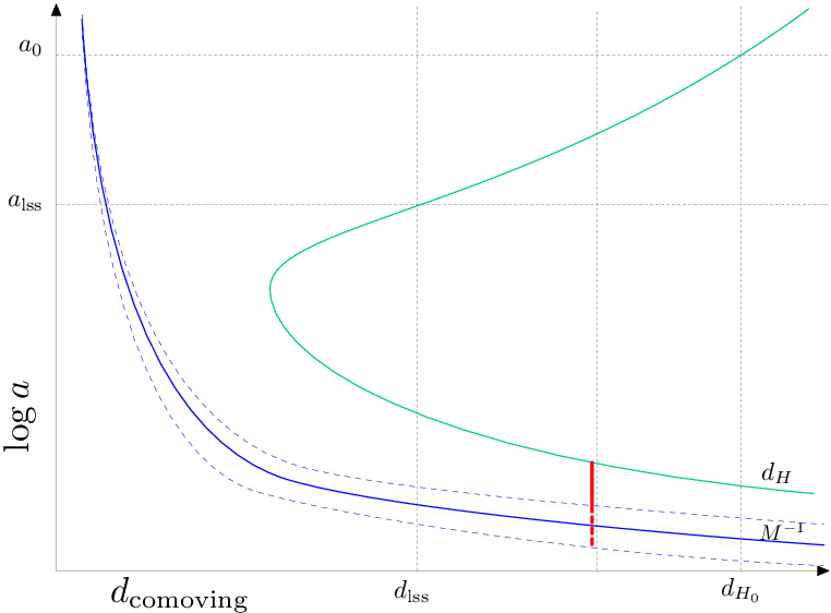
The definition of the vacuum state and the value of the power spectrum are both given in terms of the corresponding family of positive frequency solutions (hereafter called ) of the mode equation
| (9) |
Here, is the conformal time defined by and the conformal frequency whose properties will be discussed below. The initial state is defined as the state annihilated by the destruction operators associated with the modes . These operators are given by the Klein-Gordon overlap with the field operator
| (10) |
Straightforward algebra gives the power spectrum of Eq. (6):
| (11) |
As in any vacuum state, it is given by the square of the norm of the corresponding positive frequency modes evaluated long after horizon crossing.
The standard spectrum also belongs to this class. It is obtained when using the asymptotic vacuum, often called the Bunch-Davis vacuum BunchDavis. This state is defined by the solutions of Eq. (9) with positive frequency in the asymptotic past. Using the fact that for (see Eq. 19 below), the asymptotic positive frequency modes obey
| (12) |
The corresponding power spectrum is thus
| (13) |
In the long wavelength limit, when , the standard spectra of the metric perturbations obtained using (4) become constant and depend only on and the hierarchy of slow roll parameters which are logarithmic derivatives, and (we adopt the definition of beyondSL in terms of the logarithmic derivatives of instead of the logarithmic derivatives of the inflaton potential). In the slow-roll approximation, and are constants and . In addition, the long wavelength limit of (13) is expanded to linear order in . Explicitly, the gravitational wave and curvature spectra are given by (more details can be found in, e.g. MS1)
| (14) |
where , is the pivot-scale around which the expansion in is carried out, and the values of are taken when crosses the horizon.
Since the modes and obey the same equation, they are related by a time-independent transformation
| (15) |
As usual, the Bogoliubov coefficients and are given by the overlaps of the two sets of modes
| (16) |
Using these coefficients and (13) in the long wavelength limit, the power spectrum (11) is
| (17) |
This equation holds whenever new physics expresses itself through the replacement of the asymptotic vacuum with a new vacuum state. (It also applies for modified mode equations (19) including dispersion above np1, see also MB03.)
At this point, an important remark must be made. In Eq. (17), the second term in the brackets is independent of the phase conventions of the modes and . Indeed, a change and gives and , from which follows the invariance of . In other words, the phase of this term is physically meaningful. Moreover, it will play a key role in the averaging process discussed below.
The corrections in (17), whose properties will now be explained, result from the fact that the vacuum is less adiabatic than the asymptotic vacuum. Consider, for instance, positive frequency modes obeying
| (18) |
at the time defined by Eq. (5). To characterize the degree of adiabaticity, we specialize to slow-roll inflation. In this case, the conformal frequency of metric perturbations is of the form
| (19) |
where is a constant of order unity whose explicit expression is not needed here. In the above equation, we have chosen the arbitrary additive constant in conformal time such that
| (20) |
The degree of adiabaticity of the modes is controlled by the ratio np1
| (21) |
Applied to (19), it shows that the evolution is adiabatic for , i.e. when the wavelength is much smaller than the Hubble radius . Furthermore, the asymptotic evolution is WKB exact, i.e. there is no asymptotic contribution to the coefficient . Therefore, if , the positive frequency modes of Eq. (18) hardly differ from the asymptotic modes since the magnitude of the corrections is controlled by some power of the small quantity .
| (22) |
Hence the norms of the Bogoliubov coefficients (16) are
| (23) |
where and the second equality follows from (15) and unitarity.
When using the vacuum associated with the solutions of Eq. (18), one finds NPC1. If one chooses instead the solutions defined by , one obtains MB03, while those obeying yield Danielsson. This hierarchy is explained by the property that the corresponding states are instantaneous ground states at of Hamiltonians of decreasing degree of adiabaticity Veneziano. Hence, from a phenomenological point of view, the values of and should be conceived as free parameters characterizing the departure from the standard power spectrum.
Let us now consider the leading correction to the power spectrum in this class of models. For , it is always given by the second term of (17) which is linear in the coefficient . The crucial point is that its phase is universally given by
| (24) |
To derive this result, we first recall that the phase of the standard mode is calculated in the long wavelength limit, , while the phases of and of Eqs. (16) are time independent. They depend parametrically on the -crossing time since the positive frequency modes are defined at that time. The result (24) is therefore governed by the behavior of the modes in the two asymptotic regimes and .
First, in the long wavelength limit, the phase of the standard mode tends to a constant. This can be seen from the asymptotic behavior of the solution to (9) in the slow roll approximation
| (25) |
where is real and depends on the slow roll parameters and . Hence makes an -independent constant contribution to the phase (24).
Second, well inside the horizon the modes are close to Minkowski plane waves. Given their definition in Eq. (16), the phase of , i.e., the relative phase of and , is necessarily . To show this, it is sufficient to expand the solution in powers of ,
| (26) |
and notice that its time derivative can be factorized as
| (27) |
We consider the class of positive frequency modes that satisfy at time
| (28) |
where is a real number, and is a function of the form
| (29) |
For specific examples, see the paragraph below (23).
Using Eq. (27) evaluated at and Eq. (28), we get
| (30) | |||||
where obeys with defined in (23). It is related to the parameters as follows. If , it is equal to , if and it is equal to , and so on (recall that ). In the second line, we used the liberty to choose the overall phase of to set it equal to that of at (see the remark below Eq. (17)). In the last line we used Eq. (29). The coefficient is evaluated along the same lines:
| (31) | |||||
where is a complex number whose phase originates from the correction terms and which is therefore practically independent of and . The result (24) follows from the combination of Eqs. (26), (30) and (31).
The phase shift (24) has a simple physical interpretation: it is (twice) the phase accumulated from the creation time until some time long after horizon exit when the power spectrum is evaluated and the phase of the standard modes freezes out. Compared with the Bunch-Davis vacuum, the state contains pairs of quanta created at the time . The fact that quanta are created in pairs is reflected in the factor of two of the phase of the coefficient mapa. Notice also that the phase shift is approximatively the redshift factor between the two scales and , i.e., between the creation time and the time of horizon exit. This can be seen from
| (32) |
where we used that in the slow roll approximation , so that changes by a constant of order unity during the e-folds from to .
In summary, the correction to the power spectrum is the sum of two terms. A square, which we call the steady term, and an interference term that depends on through its phase, called the oscillatory correction. The steady correction is subleading and given by
| (33) |
while the oscillatory correction is the leading correction and given by the real part of
| (34) |
This term produces a modulation of the power spectrum. Indeed, using (8) and which is valid in the slow-roll approximation, one gets
| (35) |
From this we deduce that the period of the oscillations of the power spectra in -space is given by
| (36) |
It is linear in , but also inversely proportional to the first slow roll parameter . Hence, its magnitude is determined by a competition between the inflationary background evolution and the value of .
Before determining the impact of averaging over fluctuations of the scale , we present a general expression for possible deviations of the primordial power spectrum.
III A generalized Ansatz
In the previous section, we considered the particular class of models where a prescription for the vacuum state is given at some finite time. These are parameterized by only one dimensionless quantity, namely , which controls both the phase and the amplitude of the correction terms. There is, however, no reason to assume this will be always the case when dealing with a fundamental theory. We therefore consider the more general expression of modifications
| (37) |
where is a fiducial scale.
In writing this Ansatz, we assume that the deviations from new physics are constrained to mild departures from scale invariance. In other words, we do not account for phenomena that induce either sharp features (i.e., in the form of ) or rapidly oscillatory behavior such as . What motivates our choice is the fact that standard physics is nearly scale invariant, in that the deviations of the power spectrum from scale invariance only come from the background geometry through logarithmic derivatives of . This follows from the near-stationarity of the amplification process of successive modes with increasing conformal scale . Hence, under the assumption that the new physics preserves this stationarity, the -dependent corrections are still governed by as it was the case in Eqs. (II).22 2 Anticipating Section V, it is interesting to notice that sharp modifications of the primordial power spectrum (in the sense that they vary much more rapidly than ) are strongly broadened and damped by the geometric projection involved in computing the angular power spectrum of the CMB featuresinCMB. Hence, from the point of view of confronting CMB data they need not be considered.
The modified power spectrum (37) is described by new parameters. The terms proportional to and represent the oscillatory and the steady corrections, respectively. The model of Section II is contained in (37), with the special values and as seen from (33)-(II). The other coefficients can be obtained by Taylor expanding in powers of around the fiducial point , see for instance MB03 for detailed expressions. The Ansatz (37) also includes extensions of these models which allow for a so-called -vacuum in place of the adiabatic vacuum (the transformation (15) is combined with a second Bogoliubov transformation). These power spectra are considered, for instance, in MR and MB03 and are described by three independent parameters.
Notice also that the parameterization (37) allows for a combination of various subleading corrections (possibly characterized by several scales) to the standard slow-roll power spectra, but not necessarily of a high energy origin. This is particularly clear for the steady term whose Taylor expansion is
| (38) |
A calculation of the power spectrum beyond the slow roll approximation yields a result of the same form beyondSL
| (39) |
where the coefficients depend now on the parameters and are of order . A similar expansion holds for the power spectrum of primordial gravitational waves.
The corrections from matter loops make another contribution to the coefficient Weinberg:
| (40) |
where is a numerical factor and the renormalisation scale.
Consequently, high energy corrections of the type (38) may be hard to disentangle from non-trivial standard physics effects, such as the slow rolling background or loop contributions.
IV Stochastic averaging
To model the consequences of geometric fluctuations which might arise in quantum gravity, we treat as a fluctuating variable and calculate the power spectra after taking the average over its fluctuations. More precisely, we adopt the simplest description by assuming that is a Gaussian variable characterized by a mean and a spread
| (41) |
We also assume that the spread is much smaller than the mean
| (42) |
as in the Breit-Wigner description of long living atomic states. This requirement implies that the induced spread of the cosmological time defined at Eq. (5) is much smaller than the Hubble time evaluated at the mean time defined by . Indeed, by differentiation of the relation at fixed , we have
| (43) |
Similarly, the parameter now also exhibits some spread . Again, the ratio of this variance over the mean obeys .
To characterize the effects of the fluctuations, it will be convenient to parameterize the spread of by a power defined as follows:
| (44) |
The condition (42) now reads
| (45) |
where we have adopted the convention .
We now take the ensemble average of (17). Let us consider each term separately. The steady correction is basically unchanged because the norms of Bogoliubov coefficients are slowly varying functions of . Hence the mean value is well approximated by its former expression (33) evaluated with the mean quantity , that is
| (46) |
On the contrary, averaging over the fluctuations of in the oscillatory term (34) has a dramatic effect. Indeed, its mean value is damped by an exponential factor
| (47) |
To evaluate the prefactor in the exponential, we use again the slow roll approximation wherein . For instance, with and , we have . In any case, one has , something which increases the damping factor. For simplicity, we will take it equal to one.
Since one has , unless , that is unless ,the oscillatory term is exponentially suppressed by a large quantity. To appreciate the importance of this effect, it is instructive to compute the value of such that the damping of the oscillatory term reduces it to the subleading correction represented by the steady term. The averaged values of the oscillatory and steady corrections are of the same order for given by
| (48) |
For instance, if we choose and , we find . This is perfectly compatible with the constraint (45) which reads for these numerical values . For , the oscillatory term is so damped by the ensemble average that it becomes smaller that the steady correction (46) which thus provides the new leading deviation.
This conclusion has been reached for the models of Sec. II, but it can be readily generalized to deviations of the power spectra parameterized by (37). By assumption, the function weighing the steady term is a slowly varying function of , so that in a first approximation it may be replaced by its value at the mean , as in (46). Instead, the oscillatory term proportional to must be treated similarly to (47). That is, whenever the functions or change significantly over an interval , the ensemble average of the oscillatory term will be damped
| (49) |
where is a constant. The value of is determined by the fastest oscillating term. For instance, if is again linear in , one still finds .
In general the equality (48) will be replaced by
| (50) |
Hence, provided is not too small, the power may be rather small while the oscillatory term can still be severely suppressed.
In conclusion, unless , the oscillatory deviations of the power spectrum are strongly reduced and become subleading corrections to the averaged power spectra.
V Geometric averaging
In this section, we compare the high energy averaging of the deviations of the primordial power spectrum to the geometric averaging involved in computing the two-dimensional angular power spectrum. The contribution from scalar perturbations to the multipole of the temperature anisotropies can be written as CMBslowWeinberg
| (51) |
which nicely separates the contributions of the physics and the geometry. First, the spherical Bessel function acts as a projector on the celestial sphere, where is the angular diameter distance of the last scattering surface. For flat spatial sections, it is given by the lapse of conformal time since last scattering, i.e. .
Second, the curvature power spectrum seeds the various matter and radiation density perturbations, the evolution of which is encoded in the transfer functions . essentially describes intrinsic temperature fluctuations and the Sachs-Wolfe effect, while is due to the Doppler effect.
On large angular scales, i.e. for , where is the size of the acoustic horizon (in practice ), one can use the following asymptotic expressions of the form factor
| (52) |
In this case, as noticed in MR, the integral (51) actually performs a geometric average over the fine-structure of the primordial power spectrum. More precisely, for the power spectrum given by (37), the oscillatory deviations are damped by a power of the frequency of superimposed oscillations while the steady correction is not.
In the limit (52), the integral (51) can be done explicitly with the change of variables and with the help of
| (53) |
applied for the values and for the steady and oscillatory corrections respectively.
To simplify the expressions we set in (flat power spectrum). In this case, we find
| (54) | |||||
where is the unperturbed power spectrum. As in Eq. (37), and weigh the oscillatory and steady corrections respectively.
For the steady correction, if is not too large, is of order unity for all . Hence, as one might have expected, the projected amplitude of the (relative) steady correction does not significantly differ from its original amplitude in the power spectrum (37).
For the oscillatory corrections, we again consider the case where the oscillations have a high frequency. In this case, the parameter in (37). (We recall that in the models of section II, .) Using the Stirling formula to evaluate yields
| (55) |
Instead of finding an exponential damping as in Section IV, we obtain a power law suppression governed by , in agreement with Eq. (13) in MR. Therefore, the oscillatory deviations of the primordial spectrum provides the leading correction to multipoles only if
| (56) |
One can clearly see that the geometric projection introduces a preferred conformal scale through the angular diameter distance , in contrast with the scale independence of the damping of stochastic origin, see (49).
Finally, to confront deviations originating from new high energy physics to observable data, it is also necessary to evaluate , the value of of Eq. (49) such that the damping factor from the new physics equals that from the geometric average in (55). Their equality means
| (57) |
where is a constant of order unity. In turn, this implies
| (58) |
which is the same equation as (50) with the substitution . As a consequence, unless , the oscillatory correction term is damped by a factor larger than .
VI Conclusion
The geometric and stochastic averages are cumulative, in the sense that the oscillatory correction receives a second damping factor from the integral over the wavenumbers. It multiplies the first damping factor from the average over .
However, these two averaging procedures differ in the following important way. The stochastic average is (almost) scale independent, in the sense that the oscillatory correction to the power is damped by the same factor independently of the wavenumber (almost here must be understood in the same way as the unperturbed power spectrum is almost scale invariant, that is with a slow logarithmic dependence in ).
On the other hand, the geometric average considered in the previous section is only valid for large angular scales, for which the form factors can be approximated by constants. For smaller angular scales, the ’s are oscillatory functions of with a frequency equal to the size of the acoustic horizon CMBslowWeinberg. They therefore interfere with the superimposed oscillations to the primordial power spectrum and produce potentially observable oscillations in the angular power spectrum MR. In other words, the geometric averaging depends on the angular scale while the stochastic averaging does not. It is therefore possible to distinguish them in principle.
In brief, two cases leading to different lessons can be found. If the detection of the superimposed oscillations in the CMB data are confirmed, this would constitute a very strong constraint on the width of the scale . If instead the damping of the oscillatory term is so strong that the steady term becomes the leading correction, no further damping would be introduced by the geometric averaging, and the corrections would be proportional to . This may well be too small to make them observable.
Finally, as noticed in Section III, the steady corrections to the power spectra receive contributions from various physical effects. Lifting the induced degeneracy which impedes the access to information about Quantum Gravity is a challenge for future work.
Acknowledgements.
The work of DC and JCN was supported by the Alfried Krupp Prize for Young University Teachers of the Alfried Krupp von Bohlen und Halbach Foundation.References
- (1) WMAP Collaboration (D.N. Spergel & al.), astro-ph/0603449.
- (2) J. Martin and C. Ringeval, JCAP 0608, 009 (2006).
- (3) T. Jacobson, Phys. Rev. D 44, 1731 (1991); ibid. D 48, 728 (1993); W.G. Unruh, ibid. D 51, 2827 (1995); R. Brout, S. Massar, R. Parentani, P. Spindel, ibid. D 52, 4559 (1995); S. Corley, T. Jacobson, ibid. D 54, 1568 (1996); S. Corley, ibid. D 57, 6280 (1998).
- (4) J. Martin, R.H. Brandenberger, Mod. Phys. Lett. A 16 999 (2001); J. Martin, R.H. Brandenberger, Phys. Rev.D 63, 123501 (2001); J.C. Niemeyer, ibid D 63, 123502 (2001).
- (5) T. Jacobson, Prog. Theor. Phys. Suppl. 136, 1 (1999).
- (6) J. Martin and C. Ringeval, Phys. Rev. D 69, 083515 (2004); ibid 69, 127303 (2004).
- (7) J. Martin, R. Brandenberger, Phys. Rev. D 68 063513 (2003).
- (8) C. Barrabès, V.P. Frolov, R. Parentani, Phys. Rev. D 59, 124010 (1999); ibid. D 62, 044020 (2000).
- (9) R. Parentani, Phys. Rev. D 63, 041503 (2001); Int. J. Theor. Phys. 41, 2175 (2002), for an updated version see [arXiv:0704.2563].
- (10) B.L. Hu and K. Shiokawa, Phys. Rev. D 57, 3474 (1998); G. Amelino-Camelia, Lect. Notes Phys. 669, 59 (2005); R. Aloisio, A. Galante, A.F. Grillo, S. Liberati, E. Luzio, and F. Méndez, Phys. Rev. D 74, 085017 (2006).
- (11) R. Easther, B. R. Greene, W. H. Kinney, G. Shiu, Phys. Rev. D 66, 023518 (2002).
- (12) J. M. Bardeen, P. J. Steinhardt, and M. S. Turner, Phys. Rev. D 28, 679 (1983); J. Martin and D.J. Schwarz, Phys. Rev. D 57, 3302 (1998); D. Wands, K. A. Malik, D. H. Lyth, and A. R. Liddle, Phys. Rev. D 62, 043527 (2000).
- (13) V.F. Mukhanov, H.A. Feldman, and R.H. Brandenberger, Phys. Rep. 215, 203 (1992).
- (14) T. S. Bunch and P. C. W. Davies, Proc. R. Soc. London A 360, 117 (1978).
- (15) D.J. Schwarz, C.A. Terrero-Escalante, A.A. Garcia, Phys. Lett. B 517, 243 (2001).
- (16) J. Martin and D.J. Schwarz, Phys. Rev. D 62, 103520 (2000).
- (17) J.C. Niemeyer and R. Parentani, Phys. Rev. D 64, 101301 (2001).
- (18) J.C. Niemeyer, R. Parentani and D. Campo, Phys. Rev. D 66, 083510 (2002).
- (19) Ulf H. Danielsson Phys. Rev. D 66, 023511 (2002).
- (20) V. Bozza, M. Giovannini, G. Veneziano JCAP 0305, 001 (2003); M. Giovannini, Class. Quant. Grav. 20, 5455 (2003).
- (21) S. Massar and R. Parentani, Nucl. Phys. B 513, 375 (1998).
- (22) W. Hu and T. Okamoto, Phys. Rev. D 69, 043004 (2004).
- (23) S. Weinberg, Phys. Rev. D 72, 043514 (2005); ibid. 74, 023508 (2006).
- (24) S. Weinberg, Phys. Rev. 64, 123512 (2001); V.F. Mukhanov, Int. J. Theor. Phys. 43, 623 (2004).