Scalar field confinement as a model for accreting systems
Abstract
We investigate the possibility to localize scalar field configurations as a model for black hole accretion. We analyze and resolve difficulties encountered when localizing scalar fields in General Relativity. We illustrate this ability with a simple spherically symmetric model which can be used to study features of accreting shells around a black hole. This is accomplished by prescribing a scalar field with a coordinate dependent potential. Numerical solutions to the Einstein-Klein-Gordon equations are shown, where a scalar filed is indeed confined within a region surrounding a black hole. The resulting spacetime can be described in terms of simple harmonic time dependence.
I Introduction
Self-gravitating scalar field configurations have been very useful in many aspects of gravitational theory. Their role as describing matter models (eg.MTW; scheelteuk; kaup; ruffini; seidelsuen); as governing mechanisms to model inflationary scenarios (eg. liddle; Lidsey:1995np); as probes of strong curvature regions (eg.choptuik; Gundlach:1997wm), etc. has made them an ideal tool in a number of fronts. In this work we examine exploiting scalar fields to mimic some salient properties of accreting black hole systems. To this end, it is desirable to explore a configuration where the scalar field simulates an accretion disk surrounding a black hole. For this purpose, one should be able to confine the scalar field within some compact region surrounding the black hole. Since massless scalar fields radiate away to infinity, the model sought after should include a mechanism that will prevent this from happening, at least to some non-trivial extent. (The existence of bound states for particular cases in spherical symmetry are studied in bound; bound2).
One way to confine the scalar field would be by employing a potential well which would introduce some sort of barrier and thus allow for confinement. The use of carefully chosen potentials is common practice with scalar fields, and are usually functions of the field itself. Examples of this kind of potential are the quadratic () –that introduces a mass term–; and the quartic (). However, that kind of potential does not allow for confining the scalar field within a specific region of space, that one can specify a priori.
What we are looking for is a potential that somehow depends on the coordinates and in particular can be chosen to describe a potential well within a region. However, this proposition seems a priori at odds with maintaining covariance. The difficulty one encounters with a coordinate-dependent potential, is that the corresponding stress-energy tensor is in general inconsistent, in the sense that its divergence will not be zero for a non-trivial scalar field. This fact, together with the Einstein equations, would imply that the Bianchi identities are not satisfied.
Faced with this situation a possible way of confining the scalar field would be to introduce a background with respect to which coordinates could be defined. This approach would be in line with bi-metric theories of gravity (eg.rosen). Another approach would be to fix a suitable coordinates already at the level of the action as is done in kuchar through some suitably introduced Lagrande multipliers. This procedure then provides a way to convariantly adopt coordinates which could, in principle, be used in the potential. However, this method would strongly link the adopted gauge with the type of potential introduced and it is not yet clear whether it can be made of practical use. An alternative way, which is the one we pursue here, is to exploit symmetry considerations without resorting to introducing any other feature in the problem. The existence of the symmetry provides a simple way to consistently introduce a coordinate-dependent potential in the problem. Certainly, while more restricted than other possible viable options, this approach is the more direct one. A particular case of a coordinate dependent potential has already been implemented in frans; unpub to effectively simulate angular momentum in spherical or axial symmetry.
In this work we concentrate mainly on the case of spherical symmetry, but give prescriptions for the implementation of potentials in both spherical and axial symmetry. We will see that, if the space is spherically symmetric, we can implement a potential that depends on the areal radius. In the same way, for an axially symmetric spacetime, the potential can depend on the length of the closed integral curves defined by the associated killing vector. Even though one will not be able to specify the potential as an arbitrary function of any coordinate, one may still be able to confine a scalar field to some region, as is it shown in this work for the case of spherical symmetry. This fact will become apparent in section II.1 and in its applications in the rest of this work.
This paper is organized as follows. In section II, we study the specification of a stress-energy tensor for a scalar field with a coordinate dependent potential. Showing that such implementation is possible when the space-time possesses a symmetry. In particular, the case of spherical symmetry is studied in depth (we also consider an axi-symmetric case in an appendix). In section III we describe the formulation used, and the resulting equations. In section IV we discuss how the equations are solved numerically, after obtaining initial data by two different methods. In section V we show and analyze the numerical solutions obtained, finding that, after some transient behavior, the scalar field reaches a state described by a simple harmonic time dependence and remains confined to a region surrounding the black hole. We have confirmed these for initial masses of the scalar field up to of that of the black hole. Finally, we make some final remarks in section VI. In all this work we use Einstein’s index notation and geometrized units.
II Scalar Field on a Coordinate-Dependent Potential
In this section we study the specification of a stress-energy tensor for a scalar field with a coordinate dependent potential. Our motivation is to somehow confine a scalar field within a region around a black hole. The resulting system would share features of a black hole interacting with an accretion disk. We will see that this can be done when the space-time posses a symmetry. However, the specification of such potential is not completely arbitrary since it must depend on the coordinates only through some particular function. Knowing the approximate dependence of that function on the coordinates, one can then construct a potential that confines the scalar field.
Before presenting our approach, we include an overview of how the equations of motion are obtained from a stress-energy tensor in the case of a coordinate-independent potential. Then, based on that procedure, we will study the generalization to the case of a coordinate-dependent potential.
The equations of motion for a real scalar field on a coordinate-independent potential can be derived from the stress-energy tensor
| (1) |
where, for later convenience, we have split this tensor into what we call the “kinetic” and “potential” terms:
| (2) |
| (3) |
The kinetic part, , corresponds to a massless scalar field without a potential.
The equations of motion can be obtained wald; MTW through the condition
| (4) |
which must be satisfied to be consistent with a covariant theory. Equation (4) can be re-expressed with as a common factor,
| (5) |
where contains second order derivatives of . The equations of motion for a non-trivial scalar field is then
| (6) |
For example, for we obtain the Klein-Gordon equation,
| (7) |
This is analogous to the Lagrangian approach, where the variation of the
action is set to zero, and, after integrating by parts, the integrand becomes
.
After this detour, we now turn our attention back to the case of interest, the implementation of a coordinate-dependent potential. Our discussion is based on the precedent one though now generalizing it to the case of a coordinate-dependent potential .
A naive first approach would be to replace occurrences of in (3) by . However, this will bring an unfortunate consequence, namely that one can now no longer express the divergence of in the form given by eqn (5), where appears as a common factor. Instead one has
| (8) | |||||
The crucial difference with eqn. (5) is that several (independent) equations must be satisfied by the real scalar field . As a result, the system of equations will be generically inconsistent.
To resolve this problem we start by: (i) adopting a different ansatz for (equation (9) below), and (ii) imposing symmetry conditions on the scalar field.
First, consider setting , instead of being given by equation (3), to be the product of a function of and a coordinate dependent tensor,
| (9) |
where the function is independent of and the tensor is independent of . Now, find a suitable such that takes the form of equation (5), this will induce conditions on . Under this choice the divergence of the stress-energy tensor results
| (10) |
Now, we look for conditions that would allow us to express the r.h.s. of equation (10) in such a way that appears as a common factor. Since is independent of , cannot appear in the last term of (10); Then, that term must be zero, resulting in the first condition on ,
| (11) |
We now consider the second term in the r.h.s.; the condition
| (12) |
for some scalar , ensures that that term has as a common factor. Equation (12) is satisfied for any scalar field if
| (13) |
However, this condition, together with equation (11), implies that is a constant. This means that is of the form (3) (with independent of ). Thus, for an arbitrary scalar field, and without any further structure in the spacetime, space-dependent potentials can not be considered. However, by imposing further conditions on the scalar field , can indeed be chosen with further structure than that of equation (13) while still satisfying equation (12). To this end, we consider11 1 This equation can be thought just as the definition of the tensor the tensor of the form
| (14) |
Replacing (14) into (12) we find
| (15) |
The simplest case is the one with for which is given by (13). More general cases arise when is independent on one of the coordinates, lets say . Here one can adopt arbitrarily and set all other components to zero, thus satisfying equation (15).
In this particular case, takes the form
| (16) |
for some functions and .
Similarly, when does not depend on two of the coordinates, lets say , , one can choose
| (17) |
Analogous results are obtained when some of its derivatives are linearly
related. For example, if , one can
adopt arbitrarily and set keeping all other components
zero. With this choice, equation (15) will be satisfied and will then be given in
terms of two functions and in a slightly different way
as is (16).
Summarizing, we have seen that a coordinate dependent potential can be implemented if the following conditions are satisfied: (i) its derivatives are linearly dependent (this includes the possibility of one or more of them being zero). (ii) The “potential” part of the stress-energy tensor is given by (9), with satisfying and being expressible in the form (16), (17), or similar expressions depending on how condition (i) is fulfilled.
In the next section we will consider in detail the case of spherical symmetry.
II.1 Spherical Symmetry
We will now concentrate on the case of spherical symmetry. The line element can be written in the form
| (18) |
where , , , and are functions of and . We assume that we can adopt coordinates so that . Then, is given by (17), with the additional condition that due to the spherical symmetry. is then
| (19) |
with and functions of and .
The evaluation of gives rise to non-trivial equations only on the and components,
| (20) | |||||
| (21) |
In order to obtain a family of solutions to these equations we will demand that depends on the coordinates only through : . With this condition, we have that
| (22) |
for . Substituting this into either equation (20) or (21), we obtain an expression for in terms of ,
| (23) |
We have just seen that, if depends on the coordinates only through , and is given in terms of by (23), the prescription (19) for the tensor allows us to express with as a common factor. More explicitly:
| (24) |
Notice that, if one wanted to calculate without setting at the onset, one would obtain (24), but with replaced by for the angular components and . However, because those terms are actually multiplied by zero, equation (24) is true for all four components.
Setting the r.h.s of (24) to zero we obtain the equation of motion for ,
| (25) |
where we remind the reader that is an arbitrary function of , and is an arbitrary function of .
Throughout the rest of this work we will choose these functions as
| (26) | |||||
| (27) |
We do that, so that the equation of motion for the scalar field becomes
| (28) |
where we interpret the function as a (coordinate-dependent) potential. The parameter is set to zero in our simulations. The function is just the square of the areal radius, . Then, we can write (28) in the form
| (29) |
where is an arbitrary function of the areal radius.
In appendix A we summarize the results obtained in the case of axial symmetry.
III The Equations
In this work we solve the non-vacuum Einstein equations for a dynamic spherically symmetric space time, coupled to a real scalar field. The scalar field satisfies a Klein-Gordon-like equation with the addition of a potential, as explained in section II.1.
The equations are decomposed using a Cauchy formulation, in which the space-time is foliated by space-like surfaces. The particular formulation used is the Einstein-Christoffel hyperbolic formulation york_fixing, where the equations are decomposed into a system of first order hyperbolic “evolution equations,” plus a system of (first order) “constraint equations.” These equations can be solved by giving initial data that satisfy the constraint equations on a given surface of the foliation, and then integrating the evolution equations in time. The constraint equations at later times are then automatically satisfied wald in the domain of dependence of that surface.
The equations solved are the Einstein-Klein-Gordon equations, with the addition of a potential,
| , | (30) | ||||
| , | (31) |
where the stress-energy tensor, , and the potential, , are given according to section II.1, as well as the condition that is independent of . In equation (31) we have set , but this parameter can be incorporated in the definition of .
We consider the line element and extrinsic curvature of a space time in spherical symmetry in the form
| (32) | |||||
| (33) |
where is the ( component of the) shift vector, and is the lapse function. In the Einstein-Christoffel formulation, the shift and “densitized lapse” function, , are arbitrarily specified and kept fixed during the evolution. We denote by the determinant of the three-metric.
In spherical symmetry, this system reduces to nine first order evolution equations, and four first order constraint equations, the later containing only spatial derivatives.
The variables evolved are: the metric components, and ; the scalar field, ; and other variables used to convert the equations from second to first order. They are: the extrinsic curvature components, and (defined in eqn.(33)); variables constructed with first-derivatives of ,
| (34) | |||||
| (35) |
and the variables containing first spatial derivatives of the metric,
| (36) | |||||
| (37) |
IV Numerical Implementation
IV.1 Initial Data
Consistent initial data must satisfy equations (79)-(83). These equations determine some variables in terms of others judiciously chosen. In this work, we exploit this freedom to describe a black hole centered at by specifying from the known Schwarzschild solution and solving for and .
Before describing the details of our implementation, we discuss how the potential and scalar field are chosen. We adopt a potential with two free parameters to regulate the depth and location of the “well” where the scalar field is to be confined (see figure 1). A simple expression for suffices for this task, and we adopt
| (38) |
with the areal radius given by . The parameters in this expression were set to and , where is the initial mass of the black hole. Notice that during the evolution , thus, in these coordinates, the shape (and position) of the potential well can change in time. We will return to this point later.
The scalar field is defined following either one of two different strategies. One is designed to conform to time-harmonic situations in weakly-gravitating cases and the other simply prescribing a sufficiently smooth profile. The latter choice allows us to investigate the spacetime’s response to fields not designed to conform to a time-harmonic dependence.
IV.1.1 Time-harmonic scalar field
To prescribe a scalar field which will give rise to a spacetime with harmonic time-dependence, we begin by considering the limiting case when the scalar field’s amplitude is negligible; there the metric should be described by the Schwarzschild’s solution. Now, considering the scalar field as existing over this fixed background spacetime, a Schrödinger-like eigenvalue equation can be obtained to determine time-harmonic states as discussed below.
The Schwarzschild metric in Eddington-Finkelstein coordinates is:
| (39) | |||||
We use this metric to evaluate the equation of motion for , equation (31). To solve this PDE we use the following ansatz that yields separation of variables22 2 Suggested by the fact that in Schwarzschild coordinates, (, ), the ansatz yields separation of variables. The coordinates transformation being: , .,
| (40) |
The equation for results
| (41) |
where the second order operator is given by
| (42) | |||||
Equation (41) is integrated to obtain . Then, from its definition, equation (40), is calculated. Finally, from we obtain and evaluating these functions at and adopting them as initial data.
Equation (41) can be straightforwardly integrated to obtain both the eigenvalue and eigenfunction through a standard shooting algorithm. To this end, we transform the second-order equation to a system of two first order equations for and augmented with a third equation () to simplify the implementation (see nrf for the details).
The system of equations is then integrated outwards from on one hand, and also inwards from . The obtained solutions are matched at an intermediate point, in our case at (the center of the potential well), with the conditions that both the solutions and derivatives are continuous. The initial guesses for the boundary conditions are then varied until a satisfactory match is obtained. The code used to implement the shooting algorithm is the one described in nrf, except that the ODE integrator is replaced for LSODE (Livermore Solver for ODEs) lsode. The boundary conditions, consistent with the physical scenario in mind are determined as follows.
We have a system of three first order ODEs, thus three boundary conditions need be specified. Natural conditions for our purposes result from requiring the fields fall sufficiently rapid at the boundaries. We thus impose a relationship between and its derivative at each boundary, of the form . The coefficient at each boundary can be found through a WKB-type approach. To do so, we first consider the variable change and fix so as to remove the first order derivative in equation (41). The resulting equation is
| (43) |
with and ,
| (44) | |||||
| (45) |
and we interpret as an effective potential (which is shown in figure 1).

Next, we freeze the coefficients and on a small neighborhood of each boundary point and consider solutions of the form , with . The following conditions at the boundaries are then determined by
| (46) | |||
| (47) |
where
| (48) | |||
| (49) |
As illustrated later, these conditions indeed ensure the solutions decay rapidly outside of the potential well (for a bounded range of values of ). Notice that since the equations are homogeneous there remains a freedom on the amplitude of the fields at the boundaries. We fix this freedom by setting at and adopting as the varying parameter for the shooting method the value of at .
Once obtained in using equation (40), we set outside this region. For the amplitude of used in this work in the case of time-harmonic initial data, the values of and its derivative at and are small enough to ensure that this matching is sufficiently smooth, as is corroborated when evolving these initial data.
IV.1.2 Smooth profile
The other approach employed in this work is to adopt a simple expression for the scalar field. In particular we adopt a “pulse” of compact support of the form
| (50) |
where the values and control the width of the pulse and were chosen so that it is centered with the potential (at ): , . After specifying and , the coefficient is chosen so that the scalar field has a given mass. This initial data is used to compare with the previous approach in regimes where the fixed-background approximation is justified and to study the spacetime’s behavior in non-linear cases.
Remaining data
Having specified both the potential and the scalar field, consistent initial data is determined by integrating the constraint equations in the following manner. First, the functions , , , and are set equal to those read-off from the Schwarzschild solution in Eddington-Finkelstein coordinates. Adopting these coordinates gives the freedom to place the inner boundary inside the black hole. We found it convenient to rewrite the constraint equations in the form:
| (51) | |||||
| (52) | |||||
| (53) |
where represents all the functions that are specified a priori (including ). These equations are integrated outwards from the inner boundary using the step adaptive integrator LSODE, using as boundary data (, , and at ) the values read-off from the Schwarzschild solution.
IV.2 Evolution
We discretize the equations with a scheme formulated to take advantage of numerical techniques which guarantee stability of generic linear first order hyperbolic systems. In this work we adopt: (i) second order accuracy by implementing second-order derivative operators satisfying summation by parts KS1; KS2; strand; SBP0; SBP1; (ii) a third-order Runge-Kutta operator for the time integration through the method of lines tadmor; (iii) a Kreiss-Oliger KO style dissipative algorithm to control the high frequency modes of the solution gustaffsonkreissoliger; SBP1; SBP2 and (iv) maximally dissipative boundary conditions setting all incoming modes to zero olsson; gustaffsonkreissoliger.
We employ a uniform grid to cover the region with equi-spaced points. The grid-spacing between points is . The time step is defined in terms of as and is chosen so that the CFL condition thomas is satisfied. In what follows, sub-indices denote particular points of a slice, and super-indices distinguish each slice.
The inner boundary, , is set inside the black hole initially, and monitored during the evolution to ensure that it remains inside and constitutes and outflow boundary of the computational domain. Then, there is no need to prescribe boundary conditions there. At the outer boundary, maximally dissipative boundary conditions are adopted. In our present case we take the simplest form of these conditions and set the incoming modes to zero. The characteristic structure for the system of equations is detailed in appendix C.
The code have been tested to ensure that the numerical solutions obtained converge to the corresponding solutions of the Einstein equations. In appendix D we show the convergence test for the Hamiltonian constraint.
V Analysis and Results
In the simulations performed in this work we set the initial mass of the black hole to (in geometrized units). The domain of integration was chosen so that the region of interest is unaffected by the conditions adopted at the right boundary. This corresponds to and . The maximum resolution used was (22000 grid points).
In the two approaches we use to obtain initial data, we have the freedom of adjusting the amplitude of the scalar field, which in turn determines its mass. We set initial data where the mass of the scalar field is in the time-harmonic case, while for the non-time-harmonic cases we set equal to , , ( being the initial mass of the black hole and ). To calculate the mass we use the Misner-Sharp formula MTW,
| (54) |
which measures the total mass inside a spherical surface labeled by coordinate . In our initial data the mass of the black hole, , is preset, so we can calculate by subtracting from the total mass of the space-time,
| (55) |
where labels a sphere containing the scalar field, which is localized initially. (See figure 8).
During the evolution we employ this formula, replacing for at the horizon33 3 The position of the apparent horizon is given by the outermost trapped surface..
In our analysis we also evaluate the Kretschmann invariant , where is the Riemann tensor. This quantity provides a gauge-invariant answer that can be compared with its value in known spacetimes. For a Schwarzschild space-time, is given by
| (56) |
where, in Schwarzschild coordinates, and . We evaluate the quotient using (56) with and defined in (54).
V.1 Initial Data
As explained in section IV.1.1, we first find time-harmonic states for the scalar field on a Schwarzschild space-time. By varying the initial guess for the frequency in the shooting integration we obtain different modes. We show the first modes in figures 2 and 3. However, for this work we used only the first mode which will be referred to as “the time-harmonic state”, unless otherwise specified. These modes have been re-scaled so that they can be normalized (in analogy with quantum mechanics) so that . There is no physical justification for choosing that particular normalization, but it is helpful when comparing different eigenstates, which otherwise would have greatly different amplitudes.


The other approach used to define the initial data corresponds to the “pulse” described in section IV.1.2. In the linear regime we employ both types of initial data, with a scalar field’s initial mass . In the non-linear regime we adopt only the non-time-harmonic initial data with masses ranging from to .
V.2 Evolution
We study the evolution of the prescribed data. We begin by considering first the linear regime, adopting scalar field configurations with initial mass of 1% of that of the black hole. After confirming that the time-harmonic configuration behaves as expected, we confirm that the “pulse” configuration evolves towards a time-harmonic regime. Then, we study cases in the non-linear regime, with initial scalar field masses ranging from 10% to 50% of that of the black hole. In all cases we evolve until .
Linear case
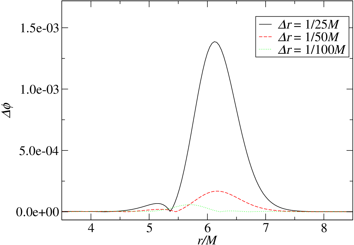
The time-harmonic initial data constructed essentially remains unchanged through the evolution while the non-time-harmonic data evolves towards a time-harmonic state. Figures 4 and 5 illustrate at different times for the maximum resolution employed (). Figure 4 corresponds to the time-harmonic initial data, and figure 5 to non-time-harmonic initial data. In both cases we sampled along two different periods at ; and then at . The corresponding pairs, are then plot together illustrating how after 22 periods apart the solutions are essentially the same.


This is further illustrated in figure 6 where we show the difference between each of these pairs for three different resolutions.

Finally, figure 7 displays the absolute value of the Fourier transform in time of , denoted . The scalar field is first integrated in space, then a discrete Fourier transform in is calculated, where ranges from to in the case of time-harmonic initial data, and from to in the non-time-harmonic case. In the plot we also indicate the frequencies () obtained from the shooting integration when calculating the time-harmonic states. The time is chosen after the initial transient behavior, indicated by a time-harmonic behavior observed in .

The initially non-time-harmonic scalar field relaxes to a superposition of the first three time-harmonic modes, the first one being the dominant one. We point out here that for this configuration, the shooting method gives raise to three possible modes. It is thus no surprising that the evolution gives rise to a solution described by these modes. Deeper potentials give rise to more modes.
Figures 8 and 9 show the Misner-Sharp mass function (equation (54)) for both types of initial data. The continuous line shows the initial value ( at ). The discontinuous lines show at for three different resolutions. In both cases the asymptotic value of the mass stays constant, indicating no scalar field energy is radiated away. An inspection of the mass behavior at smaller radii for the solution obtained with time-harmonic initial data reveals that this converges to essentially the initial value, thus a negligible amount of mass falls into the black hole. For the non-time-harmonic case about of the field’s initial mass falls into the black hole.
The amount of mass that falls into the black hole is calculated by subtracting the Misner-Sharp mass at the horizon, minus the initial mass of the black hole. In the case of time-harmonic initial data this number is , while for that of non-time-harmonic initial data it is (see table 1 and figure 14). These values are calculated using the highest resolution (), and the errors as the difference of these values with those of a lower resolution ().


Non-linear case
We turn now to the non-linear cases investigated. These correspond to initial mass configurations where the scalar field has a mass of at least 10% of that of the black hole. In this regime we solely adopt the “pulse” prescription defined in equation (50) for the scalar field since the time-harmonic data is obtained under an assumption which is no longer valid.
As we have done for the linear case, we also compare profiles at different times for simulations with higher initial . Figures 10 and 11 correspond to initial masses of the scalar field of and , respectively. The time it takes to reach a state described by a harmonic time dependence is longer than in the linear regime, especially for the higher initial . For that reason, the first samplings (labeld in the figures) occur later than in the linear case, and the interval between the profiles compared, , is ten periods, as opposed to 22 in the linear cases.


The absolute value of the Fourier transform of , , is shown in figure 12 for the two different initial masses of . Again, we compute the transformation after the initial transient behavior has passed and the scalar filed has already reached a quiescent state. As a useful indicator, we also show the frequencies corresponding to time-harmonic states. Now, while the observed modes do not coincide exactly with those obtained at the linear approximation, they are close to them.


In figure 13 we show the Misner-Sharp mass at ; and at for three different resolutions. Figures 13(a) and 13(b) correspond to initial masses of the scalar field of and , respectively. In all these cases about 10% of the scalar field’s mass falls into the black hole, while nothing escapes outwards. Additionally, for the case with grater mass, the scalar filed spreads slightly outwards before reaching a quiescent state.


Although we only show figures corresponding to two different initial values of , we have simulated the system for other values of this parameter (). In all these cases essentially no scalar field energy is radiated away, while a small portion falls into the black hole. The measured values are shown in table 1 and figure 14.
| Initial | ( |
|---|---|

If, after some transient time, the scalar field is finally confined within a compact region, lets say , the space-time should be that of Schwarzschild for , with a Schwarzschild mass equal to the total mass inside the sphere . This can be checked by evaluating the Kretschmann invariant. In figure 15 we show the quotient (see the paragraph containing equation (56)) at for the case with initial . This quotient converges to one for , and also for .

VI Conclusions
We have discussed difficulties encountered when attempting to confine a scalar field distribution within some region. The existence of a symmetry in the spacetime allows for doing so in a consistent manner. For the specific spherically symmetric case, we have given prescriptions for implementing a scalar field with a potential depending on the areal radius .
We have illustrated the viability of this approach by confining a scalar field distribution around a black hole. For our particular choice of potential and initial scalar field, the scalar field becomes totally confined after some transient time, which depends on the initial mass. During the transient, part of the scalar field accretes into the black hole, while nothing escapes to infinity. By adjusting the depth of the potential, the amount of energy that falls in can be controlled.
The approach can be exploited, an extended, to mimic situations of interest. These can range from physical studies of particular systems, to serve as a testing model for infrastructure development aimed to simulate more complex systems.
Acknowledgements.
We would like to thank M. Anderson, D. Garfinkle, C. Palenzuela-Luque, J. Pullin and R. Wald for helpful discussions as well as M. Tiglio and J. Pullin for comments and suggestions on the manuscript. This work was supported in part by NSF grants PHY-0244699, PHY-0244335, PHY0326311 and PHY0554793 to Louisiana State University. The simulations described here were performed on local clusters in the Dept. of Physics & Astronomy. L.L is grateful to the Alfred P Sloan Foundation and Research Corporation for financial support.Appendix A Coordinate-Dependent Potential in Axial Symmetry
Following chandra, we write the (general) axi-symmetric line element in the form
| (57) | |||||
where all the functions appearing here are functions of , , and , but independent of . We assume that the scalar field is independent of , and hence use as given in (16). Evaluating (and assuming that and are independent of ) we find that the -component is of the form times an expression depending on the metric functions and their derivatives. We assume that the expression multiplying is not zero, because at this moment we want to consider the case of no other symmetry other than the axial symmetry. Then, setting this component to zero, we have the condition , which, as we have seen earlier, implies that is a constant. This means that the potential will be independent of the coordinates.
Consider now the special case of axial symmetry without rotation. We can write the line element in the form
| (58) |
Evaluating , the -component this time results identically zero, and, setting the other components to zero, we have:
| (59) | |||||
| (60) | |||||
| (61) |
At this point, one can follow the same procedures as in section II.1 (compare these equations to (20) and (21)). For that reason, in this section we will just summarize the results.
Equations (59)-(61) are satisfied if, (i): depends on the coordinates only through an arbitrary function of ,
| (62) |
and (ii): is given in terms of by
| (63) |
Given these conditions, one can express with as a common factor, and, setting it to zero, obtain the equation of motion for the scalar field,
| (64) |
where and are arbitrary functions of and , respectively. On can, in particular, choose these functions as follows,
| (65) | |||||
| (66) |
Then, the evolution equation becomes
| (67) |
where we can interpret as a coordinate-dependent potential.
Appendix B The Equations
The equations of motion are
| (68) | |||||
| (69) | |||||
| (70) | |||||
| (71) | |||||
| (72) | |||||
| (73) | |||||
| (74) | |||||
| (75) | |||||
| (76) | |||||
| (77) | |||||
| (78) |
where ; dots denote derivative with respect to and primes denote derivatives with respect to ; and the “source terms” are defined in equations (84)-(88).
The constraint equations are
| (79) | |||||
| (80) | |||||
| (81) | |||||
| (82) | |||||
| (83) |
where the “source” terms are difined as
| (84) | |||||
| (85) | |||||
| (86) | |||||
| (87) | |||||
| (88) |
where (see section II.1).
Appendix C Characteristic structure
The characteristic modes and eigenvalues obtained at a surface are given by
| (89) |
Appendix D Code Tests
The standard code tests have been performed, showing that all the constraints and residuals converges to zero with order two. In figure 16 we show the Hamiltonian constraint, in the case of the strongest scalar filed studied, that with initial .
The evaluation of the constraints is a particularly important test in this work, to ensure that the implementation of a coordinate dependent potential is not breaking the covariance of the theory.

References
- (1) Misner C W, Thorne K S and Wheeler J A 1973 Gravitation, (New York: W H Freeman and Company)
- (2) Scheel M A, Shapiro S L and Teukolsky S A 1994 Phys. Rev. D 49 1894
- (3) Kaup D J 1968 Phys. Rev. 172 1331
- (4) Ruffini R and Bonazzola S 1969 Phys. Rev. 187 1767 .
- (5) E. Seidel and W. M. Suen, Phys. Rev. Lett. 66, 1659 (1991).
- (6) Liddle A R (Preprint astro-ph/9901124).
- (7) J. E. Lidsey, A. R. Liddle, E. W. Kolb, E. J. Copeland, T. Barreiro and M. Abney, Rev. Mod. Phys. 69, 373 (1997)
- (8) Choptuik M W 1993 Phys. Rev. Lett. 70 9.
- (9) C. Gundlach, Adv. Theor. Math. Phys. 2, 1 (1998) [arXiv:gr-qc/9712084].
- (10) Peres A 1960 Phys. Rev. 120 1044
- (11) Everson B L and Brill D R 1967 Bull. Am. Phys. Soc. 12 578
- (12) Rosen N 1940 Phys. Rev. 147 150
- (13) Kuchar K V and Torre C G 1991 Phys. Rev. D 44 3116
- (14) Choptuik M W, Hirschmann E W, Liebling S L and Pretorius F 2004 Phys. Rev. Lett. 93 131101
- (15) Olabarrieta I, Ventrella J, Choptuik M and Unruh W (Unpublished) Critical Bahavior in the Gravitational Collapse of a Scalar Field with Angular Momentum in Spherical Symmetry
- (16) Wald R M 1984 General Relativity (Chicago: The University of Chicago Press)
- (17) Anderson A and York J W, Jr. 1999 Phys. Rev. Lett. 82 4384
- (18) Kidder L E, Scheel M A and Teukolsky S A 2000 Phys. Rev. D 62 084032
- (19) Calabrese G, Lehner L and Tiglio M 2002 Phys. Rev. D 65 104031
- (20) Press W, Flannery B, Teukolsky S and Vetterling W 1992 Numerical Recipes in Fortran (Cambridge University Press)
- (21) Hindmarsh A C (Lawrence Livermore National Laboratory, http://www.llnl.gov/casc/odepack/)
- (22) Kreiss H O and Scherer G 1974 in Mathematical Aspects of Finite Elements in Partial Differential Equations, edited by C D Boor (New York: Academica Press)
- (23) Kreiss H O and Scherer G 1977 Tech. Rep. Dept. of Scientific Computing, Uppsala University
- (24) Strand B, 1994 Journal of Computational Physics 110 47
- (25) Calabrese G, Lehner L, Neilsen D, Pullin J, Reula O, Sarbach O and Tiglio M 2003 Class. Quant. Grav. 20 L245
- (26) Calabrese G, Lehner L, Reula O, Sarbach O and Tiglio M 2004 Class. Quant. Grav. 21 5735
- (27) Levy D and Tadmor E 1998 SIAM Journal on Num. Anal. 40 40
- (28) Kreiss H and Oliger J 1973 Methods for the approximate solution of time independent problems (Geneva: GARP Publication Series)
- (29) Gustafsson B, Kreiss H and Oliger J 1995 Time dependent problems and difference methods (John Wiley and Sons)
- (30) Lehner L, Neilsen D, Reula O and Tiglio M 2004 Class. Quant. Grav. 21 5819
- (31) Olsson P 1995 Math. Comp. 64 1035; 64 S23; 64 1473
- (32) Thomas J W 1995 Numerical Partial Differential Equations: Finite Difference Methods, Texts in Applied Mathematics 22 (New York: Springer-Verlag)
- (33) Chandrasekhar S 1992 The Mathematical Theory of Black Holes (New York: Oxford University Press)