An Eta Primer:
Solving the $U(1)$ Problem with AdS/QCD

While QCD has been unequivocally established as the theory of strong interactions, the resolution of one of its mysteries, the $U(1)$ problem, has remained somewhat unsatisfying. The $U(1)$ problem is that the Lagrangian of QCD

has, in the massless limit, a global chiral $U(1)_{A}$ symmetry, under which $q_{i}\rightarrow e^{i\theta\gamma_{5}}q_{i}$, which does not seem to be reflected in the spectrum of light pseudoscalar mesons. The formation of quark condensates $\langle\bar{q}_{i}q_{j}\rangle\approx\Lambda_{\mathrm{QCD}}^{3}\delta_{ij}$ spontaneously beaks the $U(3)_{L}\times U(3)_{R}$ symmetry of massless QCD down to a diagonal $U(3)_{V}$, which should result in nine pseudoscalar pseudogoldstone bosons. The problem is that, with masses included, chiral perturbation theory unambiguously predicts a neutral pseudoscalar meson whose mass is strictly less than $\sqrt{3}m_{\pi}$ Weinberg:1975ui. However, the true hadron spectrum contains only the regular $\pi^{0}$ (140), the $\eta$ (549), and the $\eta^{\prime}$(957), so the chiral perturbation theory bound is clearly violated.

Actually, the $U(1)$ problem is little more subtle; the $U(1)_{A}$ is anomalous, i.e. broken by quantum effects. Mathematically, while the QCD Lagrangian is invariant (except for the mass terms), the functional measure in the path integral is not, and so a chiral rotation results in

where $\tilde{G}_{\mu\nu}\equiv\frac{1}{2}\epsilon_{\mu\nu\alpha\beta}G_{\alpha\beta}$. The simplest solution of the $U(1)$ problem is then to say that the $U(1)_{A}$ symmetry is not really a symmetry at all, so there should be no corresponding pseudogoldstone boson 'tHooft:1999jc; 'tHooft:1986nc. However, from the QCD side it is hard to see how the new term in (2) could make any difference. Because it is a total derivative, any Feynman diagram involving the anomaly carries a factor of zero for total momentum. Thus, the new term does not contribute at any order in perturbation theory, and therefore the solution must be non-perturbative.

If we accept that $U(1)_{A}$ is not a symmetry, the pseudoscalar sector can be modeled in the chiral Lagrangian 'tHooft:1999jc; Nath:1980nf; Kaiser:1998ds. In full generality, the chiral Lagrangian has five free parameters, corresponding to a scale for the $U(1)$ breaking, and four decay constants characterizing the interaction strength between the $\eta$ and $\eta^{\prime}$ mesons and the $J_{\mu}^{(0)}$ and $J_{\mu}^{(8)}$ currents Nath:1980nf; Kaiser:1998ds. The number of parameters can be reduced, for example by going to the large $N_{c}$ limit, but a few parameters at least remain. In particular, none of the assumptions allow a first-principles calculation of the $\eta^{\prime}$ mass.

The first convincing resolution of the $U(1)$ problem was given by ’t Hooft 'tHooft:1976fv, who argued topological instanton configurations of the QCD vector potential can contribute to the path integral through the anomaly. The instanton contributions are suppressed by factors of $\exp(-1/g_{s}^{2})$, which can be significant only for large $g_{s}$, i.e. when QCD enters the non-perturbative regime. However, instanton calculations generically have infrared divergences, due to integrals over large instanton size, so it is impossible to use them for precise quantitative calculations. Nevertheless, they seem to be the correct qualitative solution. And, for example, using QCD sum rules Novikov:1979ux, they can be used to get a ballpark estimate of the $\eta^{\prime}$ mass ($\sim 1$ GeV).

Other non-perturbative insights into the $U(1)$ problem have come from the lattice Aoki:2006xk; DelDebbio:2004mc. Because the $\eta^{\prime}$ is critically sensitive to both quark loops and non-local field configurations, it has been a challenge to simulate. Nevertheless, the lattice has been remarkably successful in this case, and a recent estimate Aoki:2006xk puts the $\eta^{\prime}$ at $871\pm 46$ MeV, which is within 10% of the experimental value. This is absolute confirmation that QCD itself solves the $U(1)$ problem. But it is hard to get any qualitative understanding from such a purely numerical approach.

In this paper, we propose that the pseudoscalar mesons can be studied both qualitatively and quantitatively with a non-perturbative framework based on the AdS/CFT correspondence Maldacena:1997re. This framework has already produced an impressive post-diction of the meson spectrum, decay constants, and couplings Erlich:2005qh; DaRold:2005zs; Katz:2005ir. It has also led to some new insights into observations about QCD, such as vector meson dominance DaRold:2005zs, and the structure of tensor mesons Katz:2005ir. Thus, it is natural to ask whether it can say anything about the $U(1)$ mystery of QCD.

The approach to AdS/QCD we take in this paper is completely bottom up. Although the AdS/CFT correspondence began strictly as a duality between a four-dimensional conformal gauge theory and a 10-dimensional string theory, it is difficult to make any quantitative predictions about QCD from the string side. Early work, studying for example, the glueball spectrum of a large-$N$ theory Csaki:1998qr, had some success when compared to lattice results; but to study real world QCD, with three flavors and massive quarks, we would need much more information about the string dual of QCD than is currently known (see, for example Sakai:2004cn). Instead, we assume that whatever the string theory is, it must contain bulk modes dual to the various local operators of QCD. To reproduce the conformal behavior of the asymptotically free regime of QCD, these modes will propagate on a background close to Anti-deSitter space. It turns out this is enough information to reproduce a number of non-trivial quantitative predictions about QCD at low energy.

The setup is a five-dimensional space, with background metric

In pure AdS the warp factor is $w(z)=1$, but we will allow for background corrections due to deviations from conformality. The extra dimension can be thought of as energy, with small $z$ representing high energy. Thus we model the IR, where QCD is strong, by boundary conditions at a point $z_{m}\sim 1/\Lambda_{\mathrm{QCD}}$. We also impose boundary conditions at $z=0$, high energy, where QCD approaches a trivial conformal fixed point. Thus the gravity background is modeling energies between $\Lambda_{\mathrm{QCD}}$ and infinity.

For this 5-D description to be equivalent to QCD, it should reproduce QCD correlation functions of external currents. These appear as probes in the UV. For each QCD operator which couples the vacuum to these currents, there must be a corresponding field in 5D which also couples to the current. More generally, for each operator in QCD, there should be a 5D field. In our case, the currents of interest are $J_{\mu R}^{b}$ and $J_{\mu L}^{b}$, the right- and left-handed $U(3)$ currents. The corresponding fields are bulk gauge fields $A_{L}$ and $A_{R}$. The operator $\bar{q}_{i}q_{j}$ which spontaneously breaks $U(3)\times U(3)\rightarrow U(3)_{V}$ is represented by bifundamental bulk scalars $X_{ij}$. The fields X_ij have interactions and a potential. However, this potential is neither calculable nor relevant to low energy, so we simply parameterize this potential and fit to data.

To study the $U(1)$ problem, we now introduce a new complex field $Y$ to represent the square of the gluon field strength: $Y\sim G^{2}_{\mu\nu}$. We can think of the phase of $Y$ as dual to $G\tilde{G}$. We emphasize that identifying $Y$ is not important for the low energy physics, we only use it to manifest a linear representation of the symmetries. Thus our 5D Lagrangian, including all terms allowed by symmetry, is

That $X$ gets a 5D mass but $Y$ does not follows form the AdS/CFT map between masses and dimensions of operators. With these masses, the solutions to the equations of motion for $X$ and $Y$ in pure $\mathrm{AdS}_{5}$ are

These must correspond to the vacuum expectation values, $\langle\bar{q}_{i}q_{j}\rangle\sim\sigma_{ij}\sim\Lambda_{\mathrm{QCD}}^{3}$ and $\langle G_{\mu\nu}^{2}\rangle\sim\Xi\sim\Lambda_{\mathrm{QCD}}^{4}$ and to the sources $M_{q}$ and $g_{s}$. Thus the $z$-dependence of a field is seen to match the scaling dimension of the corresponding operator. In the 3-flavor case, for simplicity, we will assume that $\sigma_{ij}=\sigma\delta_{ij}$ (i.e., $\langle\bar{s}s\rangle=\langle\bar{d}d\rangle=\langle\bar{u}u\rangle)$ and use only two masses $\hat{m}=\frac{1}{2}(m_{u}+m_{d})$ and $m_{s}$.

To study this theory, we will explore the pseudoscalar excitations around the $X$ and $Y$ backgrounds.

There are of course scalar excitations as well, but these are harder to study as they are sensitive to details of the $X$ and $Y$ effective potentials. For the left and right $U(3)$ gauge fields, we will only need the axial combination $A=A_{R}-A_{L}$. The longitudinal modes of $A_{\mu}$ mix with the pions, so it is helpful to include them explicitly with the replacement $A_{\mu}\to\partial_{\mu}\varphi$. Then we get

The $0$ on $\eta^{0}$ refers to the $\tau^{0}=\frac{1}{\sqrt{6}}{\mathrm{diag}}(1,1,1)$ generator of $U(3)$, and an $8$ superscript will refer to the $\tau^{8}=\frac{1}{\sqrt{12}}{\mathrm{diag}}(1,1,-2)$ generator, in the $u,d,s$ basis. Note that we have absorbed a constant into the definition of $C$, and absorbed factors of $C$ into the definition of $\kappa$. We have also dropped $\Xi\sim\langle G_{\mu\nu}^{2}\rangle$, as it is will be a subleading power correction in everything that follows. Regardless of these conventions, it is simplest to regard Eq. (9), instead of Eq. (4), as the starting point for phenomenological analysis.

In 4D the $U(1)_{A}$ symmetry is anomalous; it is broken by quantum effects. But quantum effects in 4D correspond to classical effects in 5D, so the symmetry should be explicitly broken in 5D. In unitary gauge, this is true. But in the form (9), we have restored the symmetry with our “axion” Goldstone boson $a$. In fact the whole $U(3)_{A}$ is gauged, so there is a local symmetry under which

We can use this to set $A_{5}^{b}=0$, however it is helpful to retain these modes to simplify the calculations.

Because of the gauge symmetry, the fields $\varphi,\eta$ and $a$ are not strictly independent, but they do have different physical meanings as can be seen by introducing external sources (and notation). We define

The $U(1)_{A}$ current is normalized as

A source $J_{\mu}^{b}A_{\mu}^{b}\delta(z)$ on the UV brane leads to $\varphi^{b}\partial_{\mu}J_{\mu}^{b}\delta(z)$ after introducing $\varphi$ and integrating by parts. So the source for $\varphi$ is

Finally $\eta^{b}$ and $a$ by definition correspond to specific 4D fields, so we have

Note that we use constants $g_{\eta}$ and $g_{a}$ to normalize $J_{\eta}$ and $J_{a}$, while the normalization of $J_{\mu}$ is set by the interaction strength $g_{5}$ in the Lagrangian.

These currents help us identify our pseudoscalar fields. We see that although $\varphi,\eta$ and $a$ all mix they still have physical meanings: for a particular mode, $a$ is the “glueball” component and $\eta$ and $\varphi$ are the “quark” components of the corresponding mesonic wavefunction, with $\varphi$ related to the longitudinal mode of the axial vector field.

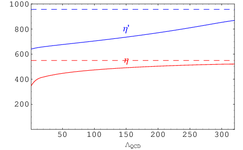
Having fit all the parameters in our Lagrangian (using only $m_{\rho},f_{\pi},m_{\pi}$ and $m_{K}$), we can now look at what masses are predicted. For the neutral pseudoscalar spectrum, there is a competition between the quark masses, which force the $\eta$ and $\eta^{\prime}$ into the $q$ and $s$ bases, and the anomaly and $\kappa$ terms, which push towards the $\eta^{0}$ and $\eta^{8}$ basis. There are seven fields, $\varphi^{0,8},\eta^{0,8},A_{5}^{0,8}$ and $a$, but we can use the residual gauge invariance to set $A_{5}^{0,8}=0$. Thus, to determine the $\eta$ and $\eta^{\prime}$ masses, we need to solve a set of five coupled differential equations. We find the smoothest numerical results if we use the equations of motion for $a,\varphi^{q},\varphi^{s},A_{5}^{q}$ and $A_{5}^{s}$, where

The equations are

with $v_{q}=m_{q}z+\sigma z^{3}$, $v_{s}=m_{s}z+\sigma z^{3}$ and $C$ given in equation (22). All the modes have Dirichlet conditions in the UV and Neumann in the IR. To canonically normalize the fields, we demand

The resulting masses are shown as a function of $\kappa$ on the left side of Figure 1. These curves are convergent, and the asymptotic values for large $\kappa$, as compared to the experimental central values (in MeV) are

So we are off by 5% and 9% respectively. We can also turn off the anomaly by lowering $\Lambda_{\mathrm{QCD}}$, as shown on the right in Figure 1.

It is worth emphasizing that taking $\kappa\to\infty$ does not send $m_{\eta^{\prime}}\to\infty$. In the chiral Lagrangian, there is a parameter like $\kappa$ which should be proportional to the anomaly 'tHooft:1999jc, and provides a mass term for the $U(1)$ pseudoscalar. In that case, taking $\kappa\to\infty$ does decouple the $\eta^{\prime}$, and the correct $\eta^{\prime}$ mass can only be reproduced by tuning $\kappa$ against the other chiral symmetry breaking terms in the Lagrangian. In AdS, we could have simply taken $\kappa=\infty$ to begin with, which would be a simpler model with $\kappa$ is replaced by a boundary condition. However, we choose to allow $\kappa$ to vary because it gives us an additional handle on the $U(1)$ sector.

Next, we calculate the decay constants. There is not a single $f_{\eta}$ and $f_{\eta^{\prime}}$. Instead, there is a decay constant for each into the $J^{0}$ and $J^{8}$ currents.

These can be calculated from the wavefunctions directly, using relations similar to those in Erlich:2005qh. For example, we solve the above differential equations with $m=m_{\eta}$, then evaluate

Similarly

So qualitatively, the $\eta^{\prime}$ is more $\eta^{0}$ and the $\eta$ more $\eta^{8}$, as expected. These values can be compared to decay constants extracted within chiral perturbation theory Feldmann:1999uf. It is, however, misleading to represent this mixing in terms of angles because the $|\eta^{0}\rangle$ and $|\eta^{8}\rangle$ components of the mass eigenstates $|\eta\rangle$ and $|\eta^{\prime}\rangle$ depend on $z$. This can be seen from Figure 2, which shows the profiles of the AdS wavefunctions of $\eta$ and $\eta^{\prime}$.

These decay constants are not directly observable. What is observable are the neutral pseudoscalar decays $P\rightarrow\gamma\gamma$, which are mediated by the axial anomaly. Amusingly, the form of this anomalous interaction in five dimensions was derived long go by Wess, Zumino and Witten (WZW) Wess:1971yu; Witten:1983tw. The bulk Chern-Simons (CS) term relevant for the decay to photons is

where $Q$ is the generator of electric charge. Here, $V_{\mathrm{AB}}$ are components of the field strength for the vector gauge field, $V_{M}(z)$, from which we want to extract the constant photon zero mode by setting $V_{\mu}(z)=1$ (this normalization is consistent with (11), see Katz:2005ir for more details about the photon). In addition to this bulk term, there is a WZW term on the IR boundary at $z=z_{m}$

which absorbs the anomaly. For constant $V_{\mu}$, with $A_{5}=0$ as usual, the CS term is a total derivative, and therefore only the boundary WZW term contributes. Explicitly, the amplitude is

which leads to (as compared to the experimental values extracted from the observed decay rates), in units of TeV^-1

These are the asymptotic values at large $\kappa$. The variation of the decay constants with $\kappa$ and $\Lambda_{\mathrm{QCD}}$ is shown in Figure 3.

We can also find the value of $\kappa$ which provides the best fit to the experimental values of $m_{\eta},m_{\eta^{\prime}},A_{\eta\gamma\gamma}$ and $A_{\eta^{\prime}\gamma\gamma}$. This is given by $\kappa=26.1$ with $m_{\eta}=466\>\mathrm{MeV},m_{\eta^{\prime}}=792\>\mathrm{MeV},A_{\eta\gamma\gamma}=30.2\>\mathrm{TeV}^{-1}$ and $A_{\eta^{\prime}\gamma\gamma}=37.3\>\mathrm{TeV}^{-1}$. The RMS error is 18%.

Now, let us turn to the topological susceptibility, $\chi_{t}$. The standard argument is that if there are massless quarks in the theory, then $\theta$ is unphysical, and thus $\chi_{t}$ must vanish. However, if all quarks are massive, or there are no quarks at all, then we expect $\chi_{t}$ to be nonzero. These facts lead the Witten-Veneziano relation Witten:1979vv; Veneziano:1979ec for the $\eta^{\prime}$ mass at large $N_{C}$

This relation, which gives $\chi_{t}=(171$ MeV)⁴, is only approximate. It assumes all the decay constants are equal, that the mesons have no glueball component, and that $N_{C}$ is large. Nevertheless, lattice seems to confirm these approximations DelDebbio:2004mc by producing $\chi_{t}=(191\mathrm{MeV})^{4}$. With our 5D construction, we can calculate the topological susceptibility, the meson masses, and the decay constants directly, and furthermore we can verify that $\chi_{t}$ vanishes only with massless quarks, from which the Witten-Veneziano relation follows.

Recall that

for a solution with $a(0)=1$. First, consider the case of pure gluodynamics. Then there are no $\eta$ or $A_{5}$ fields, and the equation of motion at zero momentum is simply

In the absence of a $\kappa$ term, it is simplest to just impose $a(z_{m})=0$ directly. Then the solution is $a(z)=1-(\frac{z}{z_{m}})^{4}=1-\frac{1}{4}(g_{a}^{2}/C^{2})\chi_{t}z^{4}$ from (60). Now suppose there are quarks. In the limit that the anomaly is weak (for example at large $N_{C}$), we can do a perturbation expansion in $C$. To leading order in $C$, the $\eta-\varphi$ system decouples from the $a$ mode. Then from (50) we get $\varphi(z)=1+\frac{1}{2}g_{5}^{2}f_{\eta}z^{2}$. Then the equation of motion (18), with $Q^{2}=-m_{\eta}^{2}$ and using (21) and (26), gives

which matches Witten-Veneziano.

To see that $\chi_{t}$ vanishes with massless quarks, we no longer assume that $C$ is small. Then the $\eta$ and $A_{5}$ equations of motion (at $Q=0$) are

If $m_{q}=0$ then the only solution for $\eta$ satisfying $\eta(0)=0$ is $\eta(z)=0$. Then $a(z)$ must be constant and the topological susceptibility vanishes. However, as long as $m_{q}\neq 0$, there is a solution with $\eta\sim z^{2}$ and $a\sim z^{4}$ near $z=0$. In this case $\chi_{t}$ is nonzero. In fact, we can solve the equations exactly for constant $C$ with $\eta(z_{m})=a(z_{m})$ boundary conditions, giving

For $C=0$ this reduces to the result from pure gluodynamics. If $C\neq 0$, then we can see directly that $m_{q}=0$ forces $\chi_{t}$ to vanish, as expected.

Note that we have not used the $\kappa$ term at all to calculate the topological susceptibility; we have only used the fact that it leads to $a(z_{m})=0$ in pure gluodynamics, or $a(z_{m})=\eta(z_{m})$ if quarks are included. The $\kappa$ term is supposed to represent some non-perturbative effects which are normally associated with instantons, so it is natural to ask if we can make the connection more precise. In QCD the one instanton contribution to the topological susceptibility can be calculated explicitly Novikov:1979ux; Geshkenbein:1979vb

Here, ${\mathcal{D}}(\rho)$ is the dilute-gas instanton density. For example, for $N_{C}=3$, ${\mathcal{D}}(\rho)=(\Lambda_{\mathrm{QCD}}\rho)^{11}$. The Bessel function ${\mathcal{K}}_{2}$ appears as the Fourier transform of $G\tilde{G}$ evaluated on a one-instanton solution. This expression is divergent due to large instantons, so one normally cuts off the integral at $\rho=\rho_{c}\sim\Lambda_{\mathrm{QCD}}^{-1}$.

In QCD it is not meaningful to compare the contribution of this specific gauge configuration to any particular calculation on the AdS side. This is because the five-dimensional dual describes only gauge invariant quantities resulting from integration over all gauge configurations, and it is not clear in which sense this particular configuration dominates the integral. Nevertheless, in truly conformal theories, where the coupling constant is a marginal parameter, it makes sense to compare non-perturbative contributions to correlators (i.e. in powers of $e^{-1/g^{2}}$) between the CFT and the five-dimensional theory. Of course, the axion would have a similar bulk description in such a case, the main difference being the $z$-dependence of the $\kappa$-like term in the dual to the CFT. We thus expect that the $\kappa$ term contribution to some correlation function to have structures similar to those one gets from integration over instanton size, since the bulk integration over the $z$-variable, must ultimately reproduce the same correlation function in the CFT.

To see the similarity to the instanton calculation, let us look at the $G\tilde{G}$ two-point function from the bulk perspective. We can solve for $a$ perturbatively around the conformal limit. In the conformal approximation, there is no IR brane, and the axion bulk-to-boundary propagator (with $a(0)=1$) is

Conformality is broken by the IR brane and by the $\kappa$ term. With these effects, the equation of motion becomes

where $\kappa(z)$ includes the non-conformal $z$-dependence of the $\kappa$ term. Now, we can get a simple expression for the topological susceptibility by integrating the action by parts on the equations of motion

If conformal invariance is a good approximation, we can estimate the effect of conformal symmetry breaking by evaluating this expression on $a^{(0)}$. We thus find

This has exactly the same form as the instanton contribution. Thus, the scale dependence of the $\kappa$ term acts just like the instanton density and the IR brane provides a natural cutoff on the integral over instanton size.

Finally, let us say a word about the QCD vacuum angle $\theta$. This angle is intimately tied to the solution of the $U(1)$ problem. The argument, roughly, is that the topological susceptibility must be nonzero to split the $\eta^{\prime}$ from the $\eta$ and the $\pi^{0}$. Since the topological susceptibility is the second variation of the effective action with respect to $\theta$, there must be sensitivity to $\theta$ in QCD. Thus the strong CP problem, which is why the apparent value of $\theta$ is so tiny ($\theta\lesssim 10^{-9}$), must be taken seriously.

In AdS, there are three angles, appearing in the $X$ and $Y$ vevs, and in the $\kappa$ term. We can write $\langle X\rangle=|\langle X\rangle|e^{i\theta_{1}}$, $\langle Y\rangle=|\langle Y\rangle|e^{i\theta_{2}}$ and $\kappa=|\kappa|e^{i\theta_{3}}$. Since $\theta_{1}$ and $\theta_{2}$ come from vevs, they can be functions of $z$ (as in Eqs.(5,6)), but $\theta_{3}$, like $\kappa$, should be a constant. In full generality, $\theta_{1}$ can have flavor indices as well. This leads to

References

- (1) S. Weinberg, Phys. Rev. D 11, 3583 (1975).
- (2) G. ’t Hooft, arXiv:hep-th/9903189.
- (3) G. ’t Hooft, Phys. Rept. 142, 357 (1986).
- (4) P. Nath and R. Arnowitt, Nucl. Phys. B 209, 251 (1982).
- (5) R. Kaiser and H. Leutwyler, arXiv:hep-ph/9806336.
- (6) G. ’t Hooft, Phys. Rev. D 14, 3432 (1976) [Erratum-ibid. D 18, 2199 (1978)].
- (7) V. A. Novikov, M. A. Shifman, A. I. Vainshtein and V. I. Zakharov, Phys. Lett. B 86, 347 (1979) [JETP Lett. 29, 594.1979 ZFPRA,29,649 (1979 ZFPRA,29,649-652.1979)].
- (8) S. Aoki et al. [JLQCD Collaborations], arXiv:hep-lat/0610021.
- (9) L. Del Debbio, L. Giusti and C. Pica, Nucl. Phys. Proc. Suppl. 140, 603 (2005) [arXiv:hep-lat/0409100].
- (10) J. M. Maldacena, Adv. Theor. Math. Phys. 2, 231 (1998) [Int. J. Theor. Phys. 38, 1113 (1999)] [arXiv:hep-th/9711200].
- (11) J. Erlich, E. Katz, D. T. Son and M. A. Stephanov, Phys. Rev. Lett. 95, 261602 (2005) [arXiv:hep-ph/0501128].
- (12) L. Da Rold and A. Pomarol, Nucl. Phys. B 721, 79 (2005) [arXiv:hep-ph/0501218].
- (13) E. Katz, A. Lewandowski and M. D. Schwartz, Phys. Rev. D 74, 086004 (2006) [arXiv:hep-ph/0510388].
- (14) C. Csaki, H. Ooguri, Y. Oz and J. Terning, JHEP 9901, 017 (1999) [arXiv:hep-th/9806021].
- (15) T. Sakai and S. Sugimoto, Prog. Theor. Phys. 113, 843 (2005) [arXiv:hep-th/0412141].
- (16) M. A. Shifman, A. I. Vainshtein and V. I. Zakharov, Nucl. Phys. B 147, 385 (1979).
- (17) L. J. Reinders, S. Yazaki and H. R. Rubinstein, Nucl. Phys. B 196, 125 (1982).
- (18) L. Randall and M. D. Schwartz, JHEP 0111, 003 (2001) [arXiv:hep-th/0108114].
- (19) T. Feldmann, Int. J. Mod. Phys. A 15, 159 (2000) [arXiv:hep-ph/9907491].
- (20) J. Wess and B. Zumino, Phys. Lett. B 37, 95 (1971).
- (21) E. Witten, Nucl. Phys. B 223, 422 (1983).
- (22) E. Witten, Nucl. Phys. B 156, 269 (1979).
- (23) G. Veneziano, Nucl. Phys. B 159, 213 (1979).
- (24) B. V. Geshkenbein and B. L. Ioffe, Nucl. Phys. B 166, 340 (1980).