Edges and Switches, Tunnels and Bridges

D. Eppstein Affiliation: Department of Computer Science, University of California, Irvine, E-mail eppstein@ics.uci.edu M. van Kreveld Affiliation: Department of Information and Computing Sciences, Utrecht University, E-mail marc@cs.uu.nl E. Mumford Affiliation: Department of Mathematics and Computer Science, TU Eindhoven, and E-mail e.mumford@tue.nl B. Speckmann E-mail speckman@win.tue.nl Affiliation: Department of Mathematics and Computer Science, TU Eindhoven, and E-mail e.mumford@tue.nl

Abstract

Edge casing is a well-known method to improve the readability of drawings of non-planar graphs. A cased drawing orders the edges of each edge crossing and interrupts the lower edge in an appropriate neighborhood of the crossing. Certain orders will lead to a more readable drawing than others. We formulate several optimization criteria that try to capture the concept of a “good” cased drawing. Further, we address the algorithmic question of how to turn a given drawing into an optimal cased drawing. For many of the resulting optimization problems, we either find polynomial time algorithms or NP-hardness results.

1 Introduction

Drawings of non-planar graphs necessarily contain edge crossings. The vertices of a drawing are commonly marked with a disk, but it can still be difficult to detect a vertex within a dense cluster of edge crossings. Edge casing is a well-known method—used, for example, in electrical drawings and, more generally, in information visualization—to alleviate this problem and to improve the readability of a drawing. A cased drawing orders the edges of each crossing and interrupts the lower edge in an appropriate neighborhood of the crossing. One can also envision that every edge is encased in a strip of the background color and that the casing of the upper edge covers the lower edge at the crossing. See Fig. 1 for an example.

Refer to caption — Figure 1: Normal and cased drawing of a graph.

If there are no application specific restrictions that dictate the order of the edges at each crossing, then we can in principle choose freely how to arrange them. Certain orders will lead to a more readable drawing than others. In this paper we formulate several optimization criteria that try to capture the concept of a “good” cased drawing. Further, we address the algorithmic question of how to turn a given drawing into an optimal cased drawing.

Definitions.

Let $G$ be a graph with $n$ vertices and $m$ edges and let $D$ be a drawing of $G$ with $k$ crossings. We want to turn $D$ into a cased drawing where the width of the casing is given in the variable $\mathit{casingwidth}$ . To avoid that the casing of an edge covers a vertex we assume that no vertex $v$ of $D$ lies on (or very close to) an edge $e$ of $D$ unless $v$ is an endpoint of $e$ . Further, no more than two edges of $D$ cross in one point and any two crossings are far enough apart so that the casings of the edges involved do not interfere. With these assumptions we can consider crossings independently. Without these restrictions the problem changes significantly—optimization problems that are solvable in polynomial time can become NP-hard. Additional details can be found in Appendix 0.A.

We define the edge crossing graph $G_{DC}$ for $D$ as follows. $G_{DC}$ contains a vertex for every edge of $D$ and an edge for any two edges of $D$ that cross. Let $C$ be a crossing between two edges $e_{1}$ and $e_{2}$ . In a cased drawing either $e_{1}$ is drawn on top of $e_{2}$ or vice versa. If $e_{1}$ is drawn on top of $e_{2}$ then we say that $C$ is a bridge for $e_{1}$ and a tunnel for $e_{2}$ . In Fig. 2, $C_{1}$ is a bridge for $e_{1}$ and a tunnel for $e_{2}$ . The length of a tunnel is ${\mathit{casingwidth}}/\sin\alpha$ , where $\alpha\leq\pi/2$ is the angle of the edges at the crossing. A pair of consecutive crossings $C_{1}$ and $C_{2}$ along an edge $e$ is called a switch if $C_{1}$ is a bridge for $e$ and $C_{2}$ is a tunnel for $e$ , or vice versa. In Fig. 2, $(C_{1},C_{2})$ is a switch.

Stacking and weaving.

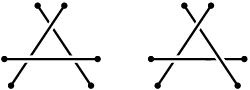
When we turn a given drawing into a cased drawing, we need to define a drawing order for every edge crossing. We can choose to either establish a global top-to-bottom order on the edges, or to treat each edge crossing individually. We call the first option the stacking model and the second one the weaving model, since cyclic overlap of three or more edges can occur (see Fig. 3).

Quality of a drawing.

Globally speaking, two factors may influence the readability of a cased drawing in a negative way. Firstly, if there are many switches along an edge then it might become difficult to follow that edge. Drawings that have many switches can appear somewhat chaotic. Secondly, if an edge is frequently below other edges, then it might become hardly visible. These two considerations lead to the following optimization problems for a drawing $D$ .

MinTotalSwitches: Minimize the total number of switches.
MinMaxSwitches: Minimize the maximum number of switches for any edge.
MinMaxTunnels: Minimize the maximum number of tunnels for any edge.
MinMaxTunnelLength: Minimize the maximum total length of tunnels for any edge.
MaxMinTunnelDistance: Maximize the minimum distance between any two consecutive tunnels.

Fig. 4 illustrates that the weaving model is stronger than the stacking model for MinTotalSwitches—no cased drawing of this graph in the stacking model can reach the optimum of four switches. For, the thickly drawn bundles of $c>4$ parallel edges must be cased as shown (or its mirror image) else there would be at least $c$ switches in a bundle, the four vertical and horizontal segments must cross the bundles consistently with the casing of the bundles, and this already leads to the four switches that occur as drawn near the midpoint of each vertical or horizontal segment. Thus, any deviation from the drawing in the casing of the four crossings between vertical and horizontal segments would create additional switches. However, the drawing shown is not a stacked drawing.

Related work.

If we consider only simple arrangements of line segments in the plane as our initial drawing, then there is a third model to consider, an intermediate between stacking and weaving: drawings which are plane projections of line segments in three dimensions. We call this model the realizable model. Clearly every cased drawing in the stacking model is also a drawing in the realizable model, but not every cased drawing in the weaving model can be realized (see [9]). The optimal drawing in Fig. 4 can be realized, hence the realizable model is stronger than the stacking model. In Appendix 0.B we show that the weaving model is stronger than the realizable model.

Results.

For many of the problems described above, we either find polynomial time algorithms or NP-hardness results in both the stacking and weaving models. We summarize our results in Table 1. In this paper we assume that our input drawing is a straight line drawing, but several of our results also generalize to curved drawings. Section 2 presents the results concerning the optimization problems that seek to minimize the number of switches and Section 3 discusses our solutions to the optimization problems that concern the tunnels. In Appendix 0.A we show that MinTotalSwitches becomes NP-hard in both the weaving and the stacking model if we allow more than three edges to cross in one point. We conclude with some open problems.

Model	Stacking	Weaving
MinTotalSwitches	open	$O(qk+q^{5/2}\log^{3/2}k)$
MinMaxSwitches	open	open
MinMaxTunnels	$O(m\log m+k)$ exp.	$O(m^{4})$
MinMaxTunnelLength	$O(m\log m+k)$ exp.	NP-hard
MaxMinTunnelDistance	$O(m\log m+k\log m)$ exp.	$O((m+K)\log m)$ exp.

Table 1: Table of results:

n

is the number of vertices,

m=\Omega(n)

is the number of edges,

K=O(m^{3})

is the total number of pairs of crossings on the same edge,

k=O(m^{2})

is the number of crossings of the input drawing, and

q=O(k)

is the number of its odd face polygons.

2 Minimizing switches

In this section we discuss results related to the MinTotalSwitches and MinMaxSwitches problems. We first discuss some non-algorithmic results giving simple bounds on the number of switches needed, and recognition algorithms for graphs needing no switches. As we know little about these problems for the stacking model, all results stated in this section will be for the weaving model.

Lemma 1

Given a drawing $D$ of a graph we can turn $D$ into a cased drawing without any switches if and only if the edge crossing graph $G_{DC}$ is bipartite.

Corollary 1

Given a drawing $D$ of a graph we can decide in $O((n+m)\log(n+m))$ time if $D$ can be turned into a cased drawing without any switches.

Proof

We apply the bipartiteness algorithm of [3]. Note that this does not construct the arrangement, so there is no term with $k$ in the runtime.∎

Define a vertex-free cycle in a drawing of a graph $G$ to be a face $f$ formed by the arrangement of the edges in the drawing, such that there are no vertices of $G$ on the boundary of $f$ . An odd vertex-free cycle is a vertex-free cycle composed of an odd number of segments of the arrangement.

Lemma 2

Let $f$ be an odd vertex-free cycle in a drawing $D$ . Then in any casing of $D$ , there must be a switch on one of the segments of $f$ .

Proof

Unless there is a switch, the segments must alternate between those that cross above the previous segment, and those that cross below the previous segment. However, this alternation cannot continue all the way around an odd cycle, for it would end up in an inconsistent state from how it started.∎

Lemma 3

Given a drawing $D$ of a graph the minimum number of switches of any cased drawing obtained from $D$ is at least half of the number of odd vertex-free cycles in $D$ .

Proof

Let $o$ be the number of odd vertex-free cycles in $D$ . By Lemma 2, each odd vertex-free cycle must have a switch on one of its segments. Choose one such switch for each cycle; then each segment belongs to at most two vertex-free cycles, so these choices group the odd cycles into pairs of cycles sharing a common switch, together with possibly some unpaired cycles. The number of pairs and unpaired cycles must be at least $o/2$ , so the number of switches must also be this large.

Lemma 4

For any $n$ large enough, a drawing of a graph $G$ with $n$ vertices and $O(n)$ edges exists for which any crossing choice gives rise to $\Omega(n^{2})$ switches.

Proof

A construction with three sets of parallel lines, each of linear size, gives $\Omega(n^{2})$ vertex-free triangles, and each triangle gives at least one switch (see Fig. 5).∎

Lemma 5

For any $n$ large enough, a drawing of a graph $G$ with $n$ vertices and $O(n^{2})$ edges exists for which any crossing choice gives rise to $\Omega(n^{4})$ switches.

Proof

We build our graph as follows: make a very elongated rectangle, place $n/6$ vertices equally spaced on each short edge, and draw the complete bipartite graph. This graph has $(n/6)^{2}$ edges. One can prove that there is a strip parallel to the short side of the rectangle, such that the parts of the edges inside the strip behave in the same way as parallel ones do with respect to creating triangles when overlapped the way it is described in the previous lemma. This gives us the desired graph with $\Omega(n^{4})$ triangles, and hence with $\Omega(n^{4})$ switches.∎

We define a degree-one graph to be a graph in which every vertex is incident to exactly one edge; that is, it must consist of a collection of disconnected edges.

Lemma 6

Let $D$ be a drawing of a graph $G$ . Then there exists a drawing $D^{\prime}$ of a degree-one graph $G^{\prime}$ , such that the edges of $D$ correspond one-for-one with the edges of $D^{\prime}$ , casings of $D$ correspond one-for-one to casings of $D^{\prime}$ , and switches of $D$ correspond one-for-one with switches of $D^{\prime}$ .

Proof

Form $G^{\prime}$ by placing a small circle around each vertex of $G$ . Given an edge $e=(u,v)$ in $G$ , let $u_{e}$ be the point where $e$ crosses the circle around $u$ and similarly let $v_{e}$ be the point where $e$ crosses the circle around $v$ . Form $D^{\prime}$ and $G^{\prime}$ by replacing each edge $e=(u,v)$ in $G$ by the corresponding edge $(u_{e},v_{e})$ , drawn as the subset of edge $e$ connecting those points.

As these replacements do not occur between any two crossings along any edge, they do not affect the switches on the edge. Both drawings have the same set of crossings, and any switch in a casing of one drawing gives rise to a switch in the corresponding casing of the other drawing.∎

In a drawing of a degree-one graph, define a polygon to be a sequence of segments of the arrangement formed by the drawing edges that forms the boundary of a simple polygon in the plane. Define a face polygon to be a polygon that forms the boundary of the closure of a face of the arrangement; note that there may be edges drawn in the interior of this polygon, as long as they do not separate it into multiple components.

Lemma 7

In a drawing of a degree-one graph, there can be no vertex on any segment of a polygon.

Proof

We have already required that no vertex can lie on an edge unless it is the endpoint of an edge. And, if a segment contains the endpoint of an edge, it cannot continue past the endpoint to form the boundary of a polygon.∎

Note, however, that a polygon can contain vertices in its interior. Define the complexity of a polygon to be the number of segments forming it, plus the number of graph vertices interior to the polygon. We say that a polygon is odd if its complexity is an odd number, and even if its complexity is an even number (see Fig. 6).

Lemma 8

Let $p$ be a polygon in a drawing of a degree-one graph. Then, modulo two, the complexity of $p$ is equal to the sum of the complexities of the face polygons of faces within $p$ .

Proof

Each segment of $p$ contributes one to the complexity of $p$ and one to the complexity of some face polygon. Each vertex within $p$ contributes one to the complexity of $p$ and one to the complexity of the face that contains it. Each segment within the interior of $p$ either separates two faces, and contributes two to the total complexity of faces within $p$ , or does not separate any face and contributes nothing to the complexity. Thus in each case the contribution to $p$ and to the sum of its faces is the same modulo two.∎

Lemma 9

Let $p$ be an odd polygon in a drawing of a degree-one graph. Then there exists an odd face polygon in the same drawing.

Proof

By Lemma 8, the complexity of $p$ has the same parity as the sum of the complexities of its faces. Therefore, if $p$ is odd, it has an odd number of odd faces, and in particular there must be a nonzero number of odd faces.∎

Lemma 10

Let $D$ be a drawing of a degree-one graph. Then $D$ has a casing with no switches if and only if it has no odd face polygon.

Proof

As we have seen, $D$ has a casing with no switches if and only if the edge crossing graph is bipartite. This graph is bipartite if and only if it has no odd cycles, and an odd cycle in the edge crossing graph corresponds to an odd polygon in $D$ . For, if $C$ is an odd cycle in the edge crossing graph, it must lie on a polygon $p$ of $D$ . Each crossing in $C$ contributes one to the complexity of this polygon. Each edge of $D$ that crosses $p$ without belonging to $C$ either crosses it an even number of times (contributing that number of additional segments to the complexity of $p$ ) and has both endpoints inside $p$ or both outside $p$ , or it crosses an odd number of times and has one endpoint inside $p$ ; thus, it contributes an even amount to the complexity of $p$ . Thus, $p$ must be an odd polygon. By Lemma 9, there is an odd face polygon in $D$ . Conversely, any odd face polygon in $D$ can be shown to form an odd cycle in the edge crossing graph.∎

Theorem 2.1

MinTotalSwitches in the weaving model can be solved in time $O(qk+q^{5/2}\log^{3/2}k)$ , where $k$ denotes the number of crossings in the input drawing and $q$ denotes the number of its odd face polygons.

Proof

Let $D$ be the drawing which we wish to case for the minimum number of switches. By Lemma 6, we may assume without loss of generality that each vertex of $D$ has degree one.

We apply a solution technique related to the Chinese Postman problem, and also to the problem of via minimization in VLSI design [2]: form an auxiliary graph $G^{o}$ , and include in $G^{o}$ a single vertex for each odd face polygon in $D$ . Also include in $G^{o}$ an edge connecting each pair of vertices, and label this edge by the number of segments of the drawing that are crossed in a path connecting the corresponding two faces in $D$ that crosses as few segments as possible. We claim that the minimum weight of a perfect matching in $G^{o}$ equals the minimum total number of switches in any casing of $D$ .

In one direction, we can case $D$ with a number of switches equal to or better than the weight of the matching, as follows: for each edge of the matching, insert a small break into each of the segments in the path corresponding to the edge. The resulting broken arrangement has no odd face cycles, for the breaks connect pairs of odd face cycles in $D$ to form larger even cycles. Therefore, by Lemma 10, we can case the drawing with the breaks, without any switches. Forming a drawing of $D$ by reconnecting all the break points adds at most one switch per break point, so the total number of switches equals at most the weight of the perfect matching.

In the other direction, suppose that we have a casing of $D$ with a minimum number of switches; we must show that there exists an equally good matching in $G^{o}$ . To show this, consider the drawing formed by inserting a small break in each segment of $D$ having a switch. This eliminates all switches in the drawing, so by Lemma 10, the modified drawing has no odd face polygons. Consider any face polygon in the modified drawing; by Lemma 9 it must include an even number of odd faces in the original drawing. Thus, the odd faces of $D$ are connected in groups of evenly many faces in the modified drawing, and within each such group we can connect the odd faces in pairs by paths of breaks in the drawing, giving a matching in $G^{o}$ with total weight at most equal to the number of switches in $D$ .

The number of vertices of the graph $G^{o}$ is $O(q)$ , where $q$ is the number of odd face polygons in $D$ . We can construct $G^{o}$ in time $O(qk)$ where $k$ is the number of crossings in $D$ by using breadth-first search in the arrangement dual to $D$ to find the distances from each vertex to all other vertices. A minimum weight perfect matching in a complete weighted graph with integer weights bounded by $k$ can be found in time $O(q^{5/2}\log^{3/2}k)$ using the algorithm of Gabow and Tarjan [5]. Therefore the time for this algorithm is $O(qk+q^{5/2}\log^{3/2}k)$ .∎

3 Minimizing tunnels

In this section we present three algorithms that solve MinMaxTunnels, MinMaxTunnelLength, and MaxMinTunnelDistance in the stacking model. We also present algorithms for MinMaxTunnels and MaxMinTunnelDistance in the weaving model. MinMaxTunnelLength is NP-hard in the weaving model.

3.1 Stacking model

In the stacking model, some edge $e$ has to be bottommost. This immediately gives the number of tunnels of $e$ , the total length of tunnels of $e$ , and the shortest distance between two tunnels of $e$ . The idea of the algorithm is to determine for each edge what its value would be if it were bottommost, and then choose the edge that is best for the optimization to be bottommost (smallest value for MinMaxTunnels and MinMaxTunnelLength, and largest value for MaxMinTunnelDistance). The other $m-1$ edges are stacked iteratively above this edge. It is easy to see that such an approach indeed maximizes the minimum, or minimizes the maximum. We next give an efficient implementation of the approach. The idea is to maintain the values of all not yet selected edges under consecutive selections of bottommost edges instead of recomputing it.

We start by computing the arrangement of edges in $O(m\log m+k)$ expected time, for instance using Mulmuley’s algorithm [8]. This allows us to determine the value for all edges in $O(k)$ additional time.

For MinMaxTunnels and MinMaxTunnelLength, we keep all edges in a Fibonnacci heap on this value. One selection involves an extract-min, giving an edge $e$ , and traversing $e$ in the arrangement to find all edges it crosses. For these edges we update the value and perform a decrease-key operation on the Fibonnacci heap. For MinMaxTunnels we decrease the value by one and for MinMaxTunnelLength we decrease by the length of the crossing, which is ${\mathit{casingwidth}}/\sin\alpha$ , where $\alpha$ is the angle the crossing edges make. For MinMaxTunnels and MinMaxTunnelLength this is all that we need. We perform $m$ extract-min and $k$ decrease-key operations. The total traversal time along the edges throughout the whole algorithm is $O(k)$ . Thus, the algorithm runs in $O(m\log m+k)$ expected time.

For MaxMinTunnelDistance we use a Fibonnacci heap that allows extract-max and increase-key. For the selected edge we again traverse the arrangement to update the values of the crossing edges. However, we cannot update the value of an edge in constant time for this optimization. We maintain a data structure for each edge that maintains the minimum tunnel distance in $O(\log m)$ time under updates. The structure is an augmented balanced binary search tree that stores the edge parts in between consecutive crossings in its leaves. Each leaf stores the distance between these crossings. Each internal node is augmented such that it stores the minimum distance for the subtree in a variable. The root stores the minimum distance of the edge if it were the bottommost one of the remaining edges. An update involves merging two adjacent leaves of the tree and computing the distance between two crossings. Augmentation allows us to have the new minimum in the root of the tree in $O(\log m)$ time per update. In total this takes $O(m\log m+k\log m)$ expected time.

Theorem 3.1

Given a straight-line drawing of a graph with $n$ vertices, $m=\Omega(n)$ edges, and $k$ edge crossings, we can solve MinMaxTunnels and MinMaxTunnelLength in $O(m\log m+k)$ expected time and MaxMinTunnelDistance in $O(m\log m+k\log m)$ expected time in the stacking model.

3.2 Weaving model

In the weaving model, the polynomial time algorithm for MinMaxTunnels comes from the fact that the problem of directing an undirected graph, and minimizing the maximum indegree, can be solved in time quadratic in the number of edges [10]. We apply this on the edge crossing graph of the drawing, and hence we get $O(m^{4})$ time. For minimizing tunnel length per edge, we can show:

Theorem 3.2

MinMaxTunnelLength is NP-hard in the weaving model.

Proof

The reduction is from planar 3-sat, shown NP-hard by Lichtenstein [7]. The reduction is similar to the one for maximizing minimum visible perimeter length in sets of opaque disks of unit size [1]. Note that the proof implies that no PTAS exists. The reduction only uses edges that intersect two or three other edges, so restricting the number of intersections per edge to be constant leaves the problem NP-hard. Also, the number of orientations of edges is constant.

A cased drawing of a set of line segments has property (A) if every line segment has at most two tunnels at crossings with a perpendicular segment, or one tunnel at a crossing with a non-perpendicular segment. Our reduction is such that a planar 3-sat instance is satisfiable if and only if a set of line segments has a cased drawing with property (A).

We arrange a set of line segments of equal length, using only four orientations. The slopes are $-4$ , $-\frac{1}{4}$ , $+\frac{1}{4}$ , and $+4$ . If two perpendicular line segments cross, then one has tunnel length equal to the width $w$ of the casing at the crossing. If two other line segments cross, then one edge has tunnel length $w/\sin(\gamma)=2,125\cdot w$ at the crossing, where $\gamma=2\cdot\arctan(\frac{1}{4})$ is the (acute) angle between the line segments. Therefore, a cased drawing with property (A) has tunnel length at most $2,125\cdot w$ , whereas a cased drawing that does not satisfy property (A) has an edge that has tunnel length at least $3\cdot w$ . This shows the direct relation between property (A) and MinMaxTunnelLength, and provides the gap that shows that no PTAS exists.

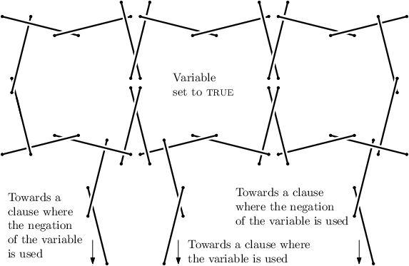
A Boolean variable $x_{i}$ is modeled by a cycle of crossing line segments as in Fig. 7. Along the cycle, crossings alternate between perpendicular and non-perpendicular, and hence it has even length. The variable satisfies property (A) iff the cycle has cyclic overlap, which can be clockwise or counterclockwise. One state is associated with $x_{i}=\,$ true, the other is associated with $x_{i}=\,$ false. In each state, the line segments of the cycle alternate in allowing an additional, perpendicular line segment to have a bridge over the line segment of the cycle. In the figure, where the cycle is in the true-state, the line segments with slope $+\frac{1}{4}$ and $+4$ allow such an extra tunnel under a line segment that is not from the cycle. If the cycle is in the false-state, the line segments with slope $-4$ and $-\frac{1}{4}$ allow the extra tunnel. We use the line segments of slope $-\frac{1}{4}$ to make connections and channels to clauses where $\overline{x_{i}}$ occurs, and the line segments with slope $+\frac{1}{4}$ for clauses where $x_{i}$ occurs. Note that the variable can be made larger easily to allow more connections, in case the variable occurs in many clauses.

Channels are formed by line segments that do not cross perpendicularly. So any line segment of the channel can have a tunnel at at most one of its two crossings, or else property (A) is violated. Note that a sequence of crossing line segments with slopes such as $-4,\,+4,\,+\frac{1}{4},\,-\frac{1}{4}$ gives a turn in the channel. The exact position of the crossing is not essential and hence we can easily reach any part of the plane with a channel, and ending with a line segment of any orientation.

A 3-sat clause is formed by a single line segment that is crossed perpendicularly by three other line segments, see Fig. 8. Property (A) holds if the clause line segment has at most two tunnels. This corresponds directly to satisfiability of the clause.

With this reduction, testing if property (A) holds is equivalent to testing if the planar 3-sat instance is satisfiable, and NP-hardness follows.∎

In the remainder of this section we show how to solve MaxMinTunnelDistance. We observe that there are polynomially many possible values for the smallest tunnel distance, and perform a binary search on these, using 2-sat instances as the decision tool.

We first compute the arrangement of the $m$ edges to determine all crossings. Only distances between two—not necessarily consecutive—crossings along any edge can give the minimum tunnel distance. One edge crosses at most $m-1$ other edges, and hence the number of candidate distances, $K$ , is $O(m^{3})$ . Obviously, $K$ is also $O(k^{2})$ . From the arrangement of edges we can determine all of these distances in $O(m\log m+K)$ time. We sort them in $O(K\log K)$ time to set up a binary search. We will show that the decision step takes $O(m+K)$ time, and hence the whole algorithm takes $O(m\log m+K\log K)=O((m+K)\log m)$ time.

Let $\delta$ be a value and we wish to decide if we can set the crossings of edges such that all distances between two tunnels along any edge is at least $\delta$ . For every two edges $e_{i}$ and $e_{j}$ that cross and $i<j$ , we have a Boolean variable $x_{ij}$ . We associate $x_{ij}$ with true if $e_{i}$ has a bridge at its crossing with $e_{j}$ , and with false otherwise. Now we traverse the arrangement of edges and construct a 2-sat formula. Let $e_{i}$ , $e_{j}$ , and $e_{h}$ be three edges such that the latter two cross $e_{i}$ . If the distance between the crossings is less than $\delta$ , then $e_{i}$ should not have the crossings with $e_{j}$ and $e_{h}$ as tunnels. Hence, we make a clause for the 2-sat formula as follows (Fig. 9): if $i<j$ and $i<h$ , then the clause is $(x_{ij}\vee x_{ih})$ ; the other three cases ( $i>j$ and/or $i>h$ ) are similar. The conjunction of all clauses gives a 2-sat formula that is satisfiable if and only if we can set the crossings such that the minimum tunnel distance is at least $\delta$ . We can construct the whole 2-sat instance in $O(m+K)$ time since we have the arrangement, and satisfiability of 2-sat can be determined in linear time [4].

Theorem 3.3

Given a straight-line drawing of a graph with $n$ vertices and $m=\Omega(n)$ edges, we can solve MaxMinTunnelDistance in $O((m+K)\log m)$ expected time in the weaving model, where $K=O(m^{3})$ is the total number of pairs of crossings on the same edge.

4 Conclusions and Open Problems

We presented polynomial time algorithms or NP-hardness results for a number of optimization problems that are motivated by cased drawings. Naturally, we would like to establish the difficulty of the MinMaxSwitches problem. We would also like to implement our algorithms to visually evaluate the quality of the resulting drawings.

References

[1] S. Cabello, H. Haverkort, M. van Kreveld, and B. Speckmann. Algorithmic aspects of proportional symbol maps. In 14th European Symposium on Algorithms, number 4168 in LNCS, pages 720–731, 2006.
[2] R.-W. Chen, Y. Kajitani, and S.-P. Chan. A graph-theoretic via minimization algorithm for two-layer printed circuit boards. IEEE Transactions on Circuits and Systems, 30(5):284–299, 1983.
[3] D. Eppstein. Testing bipartiteness of geometric intersection graphs. In Proc. 15th ACM-SIAM Symposium on Discrete Algorithms, pages 853–861, 2004.
[4] S. Even, A. Itai, and A. Shamir. On the complexity of timetable and multicommodity flow problems. SIAM Journal on Computing, 5(4):691–703, 1976.
[5] H. N. Gabow and R. E. Tarjan. Faster scaling algorithms for general graph-matching problems. Journal of the ACM, 38(4):815–853, 1991.
[6] L. J. Guibas, J. E. Hershberger, J. S. B. Mitchell, and J. S. Snoeyink. Approximating polygons and subdivisions with minimum link paths. International Journal of Computational Geometry and Applications, 3(4):383–415, 1993.
[7] D. Lichtenstein. Planar formulae and their uses. SIAM Journal on Computing, 11(2):329–343, 1982.
[8] K. Mulmuley. Computational Geometry: An Introduction through Randomized Algorithms. Prentice Hall, 1994.
[9] J. Pach, R. Pollack, and E. Welzl. Weaving patterns of lines and line segments in space. Algorithmica, 9(6):561–571, 1993.
[10] V. Venkateswaran. Minimizing maximum indegree. Discrete Applied Mathematics, 143:374–378, 2004.

Appendix 0.A Removing the restrictions

The restrictions that we impose on the input drawing—no vertex lies on a or very close to an edge, no more than two edges cross in one point, and crossing are not too close—have a significant influence on the problems that we study. For example, if we allow edges to partly overlap with vertices, then it is natural to always draw the vertex on top with a casing around it. In this case, however, there might be no cased drawing in the stacking model, because three edges that necessarily give cyclic overlap can easily be constructed. Testing if cyclic overlap occurs, and hence, if a cased drawing in the stacking model exists can be done by topological sort.

If we remove the restriction that edge crossings are not too close, we may have three edges that intersect so close that it is not possible for the edges to have a tunnel at the one crossing and a bridge at the other. Consequently, three such edges must (locally) be stacked, where one edge has a single bridge over both other edges, and both other edges have a single tunnel. Allowing such “triple crossings” makes the problem MinTotalSwitches NP-hard.

Theorem 0.A.1

If triple crossings of edges are allowed, then MinTotalSwitches is NP-hard in both the weaving and the stacking model.

Proof

By reduction from planar max-2sat shown NP-hard by [6]. Assume an instance of such a problem which has $n$ Boolean variables and $m$ clauses. The objective is to satisfy as many of the 2sat clauses as possible. We reduce the instance to an instance of cased drawing such that the number of switches is the same as the number of unsatisfied clauses in the planar max-2sat instance.

A variable is an even cycle of bundles of edges. Each bundle consists of $m+1$ parallel edges that are either horizontal or vertical. A horizontal bundle intersects two vertical bundels, and each vertical bundle intersects two horizontal bundles, see Fig. 10. Since the variables part of the construction is bipartite, it need not contain any switches. Either all horizontal edges are on top of the vertical ones, or vice versa. This corresponds to the true and false assignment of the variable, respectively.

We tap off a channel from a variable construction with a single vertical edge as in Fig. 10. The edge crosses all edges of a horizontal bundle, and to avoid switches, it must be below or above all of them (depending on whether the vertical edges in the variable are below or above). The channel itself is a sequence of single edges that leads from the variable construction to a clause construction. A channel has no switches if the edges alternate in having bridges at both crossings and having tunnels at both crossings. The parity of the number of edges in a channel determines if the channel arrives at a clause with an edge that already has a tunnel, or with an edge that already has a bridge. By using horizontal, vertical, and diagonal edges, we can always get the parity as desired and end with an edge in any orientation. So far, no switches are needed yet in a MinTotalSwitches cased drawing.

A clause consists of a single edge that has a triple crossing with the two channels that come from variables that occur in the clause. The clause edge itself cannot have a switch, because it only has the triple intersection. To avoid switches on the last edges of the channels, we can put the clause edge on top if both channel edges already have a tunnel, or we can put the clause edge at the bottom otherwise. If both channel edges already have a bridge, then there is no way to avoid a switch because one of the them will have to go below the other. There will be exactly one switch; in all other cases there are no switches at the clause. So we let the parity of any chain be such that the last channel edge be such that it has a bridge if the variable has a state that gives false in the clause.

The maximum number of switches needed is obviously at most $m$ , the number of clauses of the planar max-2sat instance. We used bundles of $m+1$ parallel edges in the variables to make sure that a variable cannot have a mixed state without giving at least $m+1$ switches already. If the bundles were just single edges, then with only two switches, one part of the channels can use the true state and the other part the false state of the variable, possibly satisfying many more clauses. The use of bundles prevents this possibility.

Note that the minimum number of switches will be achieved with a stacking drawing. Hence, the problem is NP-hard in both models.∎

Appendix 0.B Optimal drawing in the weaving model

Fig. 11 shows that the weaving model is stronger than the realizable model for MinTotalSwitches—no cased drawing of this graph in the realizable model can reach the optimum number of 12 switches. The reasoning is quite similar to the one employed for the construction in Fig. 4. The thickly drawn bundles of $c>12$ parallel edges must be cased as shown (or its mirror image) else there would be at least $c$ switches in each bundle. The 8 vertical and horizontal “normal” edges must cross the bundles consistently with the casing of the bundles, and this already leads to the 12 switches as drawn in this figure. Thus, any deviation from the drawing in the casing of the 16 crossings between the normal edges would create additional switches. However, the normal edges as drawn here constitute a perfect $4\times 4$ weaving which can not be realized (see [9]).