Inverse-free Berlekamp–Massey–Sakata Algorithm and Small Decoders for Algebraic-Geometric Codes
Abstract
This paper proposes a novel algorithm for finding error-locators of algebraic-geometric codes that can eliminate the division-calculations of finite fields from the Berlekamp–Massey–Sakata algorithm. This inverse-free algorithm provides full performance in correcting a certain class of errors, generic errors, which includes most errors, and can decode codes on algebraic curves without the determination of unknown syndromes. Moreover, we propose three different kinds of architectures that our algorithm can be applied to, and we represent the control operation of shift-registers and switches at each clock-timing with numerical simulations. We estimate the performance in comparison of the total running time and the numbers of multipliers and shift-registers in three architectures with those of the conventional ones for codes on algebraic curves.
Index Terms:
codes on algebraic curves, syndrome decoding, Berlekamp–Massey–Sakata algorithm, Gröbner basis, linear feedback shift-register.I Introduction
Algebraic-geometric (AG) codes, especially codes on algebraic curves, are comprehensive generalization of prevailing Reed–Solomon (RS) codes. They can be applied to various systems by choosing suitable algebraic curves without any extension to huge finite (Galois) fields. In fast decoding of such codes, Berlekamp–Massey–Sakata (BMS) algorithm [25] is often used for finding the location of errors, and the evaluation of error-values is done by using outputs of BMS algorithm with O’Sullivan’s formula [24].
RS codes have the features of high error-correcting capability and less complexity for the implementation of encoder and decoder. On the other hand, codes on algebraic curves have the issues related to the size of decoders as well as the operating speed of decoders. In particular, we notice that RS-code decoders need no inverse-calculator of the finite field (no finite-field inverter). The extended Euclidean algorithm [30] for RS codes has no divisions, and this enables us to operate compactly and quickly in calculating error-locator and error-evaluator polynomials. One inverse computation requires thirteen multiplications in practical GF and needs enormous circuit scale. Thus, it is strongly expected that the fast inverse-free algorithm for AG codes will be established, since division operations are inevitable on the original BMS algorithm. In addition, the decoder that has small circuit-size, such as the conventional RS decoder, is considered necessary.
In this paper, we propose an inverse-free BMS algorithm, and give a whole proof of its adequacy. Moreover, we propose three kinds of small-sized architectures that generate error-locator polynomials for codes on algebraic curves. We then explain our architectures with model structures and numerical examples, and show the practical operation of proposed architectures in terms of the control flow of registers and switches at each clock-timing. The performance is estimated on the total running time and the numbers of multipliers and shift-registers for all architectures.
The divisions in the original BMS algorithm appear at the Berlekamp transform [1]
| (1) |
at each -loop in the algorithm, where , , and are called minimal polynomial, auxiliary polynomial, and discrepancy at , respectively, runs over for sufficiently large , and is equal to a certain previous . Then the inverse-free BMS algorithm consists of modified Berlekamp transforms of the form
| (2) |
where is equal to a certain previous in this expression. Thus the denominator in (1) is converted into the multiplication of in (2). This version of inverse-free BMS algorithm can be proved in the comparable line of the original algorithm. However, there is a significant obstacle to apply this inverse-free algorithm to the decoders for AG codes; we have to mention the existence of unknown syndromes, namely, the lack of syndrome values to decode errors whose Hamming weights are less than or equal to even the basic , where is the Goppa (designed) minimum distance. Feng and Rao’s paper [3] originally proposed majority logic scheme to determine unknown syndromes in the decoding up to , where is their designed minimum distance . In the sequel, Sakata et al. [26] and independently Kötter [7] modified and applied Feng–Rao’s method to their decoding algorithm. If the divisions of the finite field are removed from BMS algorithm, one cannot execute the determination of unknown syndromes because of breaking the generation of candidate values of unknown syndromes for majority voting. Unfortunately, the elimination of finite-field divisions seemed to be a difficult problem in this regard. For this reason, no inverse-free algorithm for AG codes has been proposed until now.
In this research, we effectively overcome this difficulty. Namely, we decode such codes with the only known syndrome values from received code-words. So far the type and amount of errors that could be corrected if one does not determine unknown syndromes have not been clear; the well-known fact up to in Peterson-type algorithm [6], where is the genus of underlying algebraic curve, is not available for our case of BMS algorithm. We confirm that a class of generic errors [12][23] (independent errors in [5]) can be corrected up to only with syndromes from received words, where is the minimal pole order of underlying algebraic curve: for elliptic curves over arbitrary finite fields and for Hermitian curve over GF. Furthermore, we successfully obtain the approximate ratio of the generic errors to all errors in the application of Gröbner-basis theory, where is the number of elements in the finite field. It means that we can decode most of the errors without majority logic scheme and voting. Thus we can realize not only inverse-free error-locator architectures for AG codes but also avoiding complicated procedure and transmission of voting data among parts of decoders. Our method is applicable to all former architectures, and is not a go-back to the past but a real solution to construct decoders with feasible circuit-scale.

Recently, the BMS algorithm has become more important not only in decoding codes on algebraic curves but also in algebraic soft-decision decoding [8] of RS codes. Sakata et al. [22][28] applied the BMS algorithm to the polynomial interpolation in Sudan and Guruswami–Sudan algorithms [4][29] for RS codes and codes on algebraic curves. Lee and O’Sullivan [9][10] applied the Gröbner-basis theory of modules, which is related to the BMS algorithm, to soft-decision decoding of RS codes. Our method can be expected to help further structural analysis of these methods.
The rest of this paper is organized as follows. In Section II, we prepare notations, and define codes on algebraic curves. In Section III, we propose an inverse-free BMS algorithm, and state the main theorem for output of the algorithm. In the next three sections, we describe three types of small-scale error-locator architectures, i.e., inverse-free, serial, and serial inverse-free architectures; the mutual relations among them and past architectures are depicted in Fig. 1. In Section IV, we describe the inverse-free architecture, and divide it into three subsections: Subsection IV-A is an overview, Subsection IV-B deals with the technique for avoiding the determination of unknown syndromes, and Subsection IV-C is numerical simulation. In Section V, we describe the serial architecture using parallel BMS algorithm. In Section VI, we describe the serial inverse-free architectures combined with the previous methods. In Section VII, we estimate the total running time and the numbers of finite-field calculators for three and past architectures. Finally, in Section VIII, we state our conclusions. In the appendices, we prove the basics of BMS algorithm, the property of generic errors, and the main theorem of proposed algorithm.

II Preliminaries
In this paper, we consider one-point algebraic-geometric codes on non-singular plane curves over a finite field , in particular -type codes (not -type). Let be the set of non-negative integers, and let be and . We define a C curve by an equation
| (3) |
over with . Then the polynomial quotient ring consists of all the algebraic functions having no poles except at the unique infinite point . Let be a set of -rational points except . We denote the pole order of at as . For , the -linear subspace
has dimension , provided by Riemann–Roch theorem, which we assume for simplicity in this paper. Our code is defined as
As shown in [20][21], the class of C curves is sufficiently wide and contains almost all well-known plane algebraic curves that have many -rational points such as Hermitian codes. Although Miura in [21] defined a more general class rC including the Klein’s quartic curve, we consider mainly C for simplicity.
Throughout this paper, we denote as the number of correctable errors. Given a received word , where corresponding to a set of error-locations , we need to find a Gröbner basis [2] of the error-locator ideal
Then we can obtain as the set of common zeros of all the polynomials in the Gröbner basis.
For and , let
and . Moreover, for , let
and . Fig. 2 illustrates and for and ; although we defined as , it must be generalized into in the case of well-known Klein’s quartic curve, which is one of the important examples not contained in C curves; we will also take up codes on this curve later in section V. We note that if and only if for , and this is false for . Thus is uniquely expressed as
| (4) |
We denote by and define , where is defined on both and ; we remember that .
From a given received word , we calculate syndrome values for by , where we have by the definition of . Our aim is to find and with .
III Inverse-free BMS algorithm
We continue to prepare notations to describe the algorithm. The standard partial order on is defined as follows: for and , and . For , let be if there exists such an for and . Then is uniquely determined for each and if it exists. Note that from its definition. Table I illustrates for , where “” indicates the nonexistence of from a gap-number in .
Before the description of the algorithm, we introduce the important index for for updating in the algorithm. For and , we define a unique integer by , where the integer is defined by . If there is with , then since . Note that , and that exists if and only if exists with .
We define degree of uniquely by , and let . From now on, is abbreviated to . Defining, for ,
| (5) |
where “otherwise” includes the vacant case of , we call discrepancy of at . Let be the set of whose discrepancies are zero at all , and let . Then, for all , is an ideal in the ring (as proved at Proposition 1 in Appendix A). The BMS algorithm computes a Gröbner basis of for each , namely, a minimal polynomial ideal-basis with respect to the pole order . We may express the basis of for each as polynomials by (4). For sufficiently large , we have (proved at Proposition 3 in Appendix B). Then are called error-locator polynomials, and the set of their common zeros agrees with . Since the Goppa designed distance of equals , we may set
| (6) |
and can obtain by using .
![[Uncaptioned image]](0705.0286v1/Table_ll.png)
In the following inverse-free BMS algorithm, we denote the preserved condition (P) for updating formulae as follows: (P) or .
- Inverse-free BMS Algorithm
- Input
-
syndrome values for .
- Output
-
error-locator polynomials .
-
In each step, the indicated procedures are carried out for all .
- Step 0
-
(initializing) , ,
, ,
, , . - Step 1
-
(checking discrepancy) If exists and , then , else ;
moreover, . - Step 2
-
(-updating)
(11) (14) - Step 3
-
(checking termination) If , then and go to Step 1, else stop the algorithm.
In the formula (14), “” means that is defined by omitting the term of in . Then , can be represented by
and , are defined by these. We obtain through
Then in the algorithm agrees with the discrepancy of at , i.e., .
This inverse-free BMS algorithm is a novel version that eliminates the inverse calculation from the parallel BMS algorithm [16][27]. Compared with updating formulae in the original algorithm, which are later quoted at (21)–(V), we see that (11)–(Step 2) have eliminated the use of divisions, and in consequence have used . It is possible that one could remove the inverse calculation from the original (not parallel) BMS algorithm if the values of , which are actually previous values of , are registered to memory-elements; in our parallel inverse-free BMS algorithm, we can conveniently take from the coefficients of (as done in Step 1).
The following theorem confirms that is a Gröbner basis of .
Theorem 1
We have , ,
| (17) | |||
As explained at Proposition 3 in Appendix B, the integer is required as to correct up to errors. Moreover, it is well-known [3][26] that the determination of unknown-syndrome values has to be done to proceed the loops for of BMS algorithm. In our Theorem 1, as a result of division-less, “” is not generally true differently from Theorem 1 of [16], and this fact disables us from generating the candidate values of unknown syndromes for majority voting. Therefore, in our inverse-free BMS algorithm, we avoid the determination of unknown syndrome, and the loops of the algorithm are proceeded only for by using the known syndrome values obtained directly from the received word. Furthermore, we mainly consider the error-correction of generic errors [5][23] (defined in the next section). These techniques cause a slight decrease in the error-correcting capability; however, as described later in section IV-B, it does not matter in practice.

IV Inverse-free architecture
As the first of three kinds of architectures proposed in this paper, we describe inverse-free architecture, which has the plainest structure of the three.
IV-A Model structure
In this subsection, we give a direct application of the inverse-free BMS algorithm, which corresponds to Kötter’s architecture [7] of which inverse-calculators have been replaced by multipliers. To make the case clear, we describe the architecture for elliptic codes, that is, codes on elliptic curves, although we take the generality into account; we can employ it for other codes on algebraic curves without difficulty.
As shown in the model Fig. 3, the coefficients of , are arranged in a sequence of shift-registers, and those of , are arranged in another sequence. It is similar to Kötter’s architecture [7] that the proposed architecture has -multiple structure (i.e. blocks) of the architecture for the Berlekamp–Massey algorithm [1][11] of RS codes. The difference is that division-calculators in the Kötter’s architecture are replaced with multipliers in our architecture. Moreover, while the values of discrepancy are computed in the Kötter’s architecture with one multiplier and a shift-register according to definition (5), our architecture derives the values from the coefficients of with discrepancy registers and reduces the one multiplier for computing discrepancy.
In Fig. 3, we omit input and output terminals, and the initial () arrangement of the coefficients in polynomials is indicated. The number of registers in one shift-register sequence for and should be equal to the total number of coefficients in and , i.e., for ; although it might seem that there is no space for , it is made by shortening and shifting of as is increased. On the other hand, the number of shift-registers required for and is one more than that for and because of the structure of parallel BMS algorithm, and should be .
If , the switches in the discrepancy registers are closed downward to obtain the values of discrepancy , and if , they are closed upward to output the values of discrepancy at each clock. The head-coefficient registers work similarly to the discrepancy registers, and output the values of the head coefficient of . The coefficients of and are transferred from the block of to that of for . The switches A and B work according to the preserving or updating of and , i.e., “(P)” or “otherwise” in (Step 2) and (Step 2).
![[Uncaptioned image]](0705.0286v1/Table_registervalueIF.png)
Thus, one may only perform simple additions and multiplications for the values in the shift-register sequences for and to update them. On the other hand, as for and , one must not only perform additions and multiplications but also set register-values to zero, or else old disused values corrupt and . We describe this procedure in a later subsection IV-C.
This inverse-free architecture has an -multiple structure closer to Kötter’s than to the latter two architectures, and has been changed to division-free and parallel in the sense of using two types of polynomials, and , to compute discrepancy. We see in Section VII that the total number of shift-registers in our architecture is nearly the same as that in Kötter’s, i.e., the additional polynomials do not contribute essentially to the total number of registers.
IV-B Decoding of generic errors
To implement the inverse-free algorithm effectively, we concentrate on decoding generic -errors [5][23], for which the degree of error-locator polynomials is characterized by , while in general we have . In other word, the error-location is generic if and only if so-called delta set of error-locator polynomials corresponds to the first non-gaps in . Then the loops of BMS algorithm are required for to obtain the error-locator polynomials for generic -errors, while in general for all errors; these facts are proved in Appendix C. Thus we see that errors are corrected in after -updating for . The merits of this method are not only that it is inverse-free and there is no majority logic [3] but also that there are fewer loops of the BMS algorithm; we can cut it down to loops. Furthermore, this method can also be applied to Kötter’s and systolic-array architectures [16].
There are two drawbacks to this method. The first is that non-generic errors cannot be corrected. Since generic or non-generic is also defined by whether a matrix determinant or not (as shown in Appendix C), the ratio of generic errors to all errors is estimated at , under the hypothesis for the randomness of values (which is supported by numerical tests [12]). As for a practical size , the ratio is equal to . Moreover, for errors less than , the percentage of correctable errors increases since s decrease. Thus we have less effect of this drawback. The second is that the number of correctable errors is decreased for -error correctable codes . This corresponds to errors for all elliptic codes, and errors for Hermitian codes over . However, this has no serious effect on practical function; we might choose to correct errors, and the remaining error-correcting capability is available for error-detection up to errors. In the next subsection, we demonstrate the decoding of with (i.e. ) for -error correction in codes on elliptic curves.

IV-C Simulation and numerical example
In this subsection, we focus on an elliptic code, especially on the elliptic curve defined by the equation over , and simulate a decoder for it. This curve has 25 -rational points equal to the Hasse-Weil bound with genus one, and we obtain code of length 24.
We choose a primitive element of satisfying , and represent each non-zero element of as the number of powers of . Moreover, we represent zero in as ; note that, e.g., 0 and mean and 0, respectively. Let the set of error-locations , and let the error-values be 6, 8, 11, respectively.
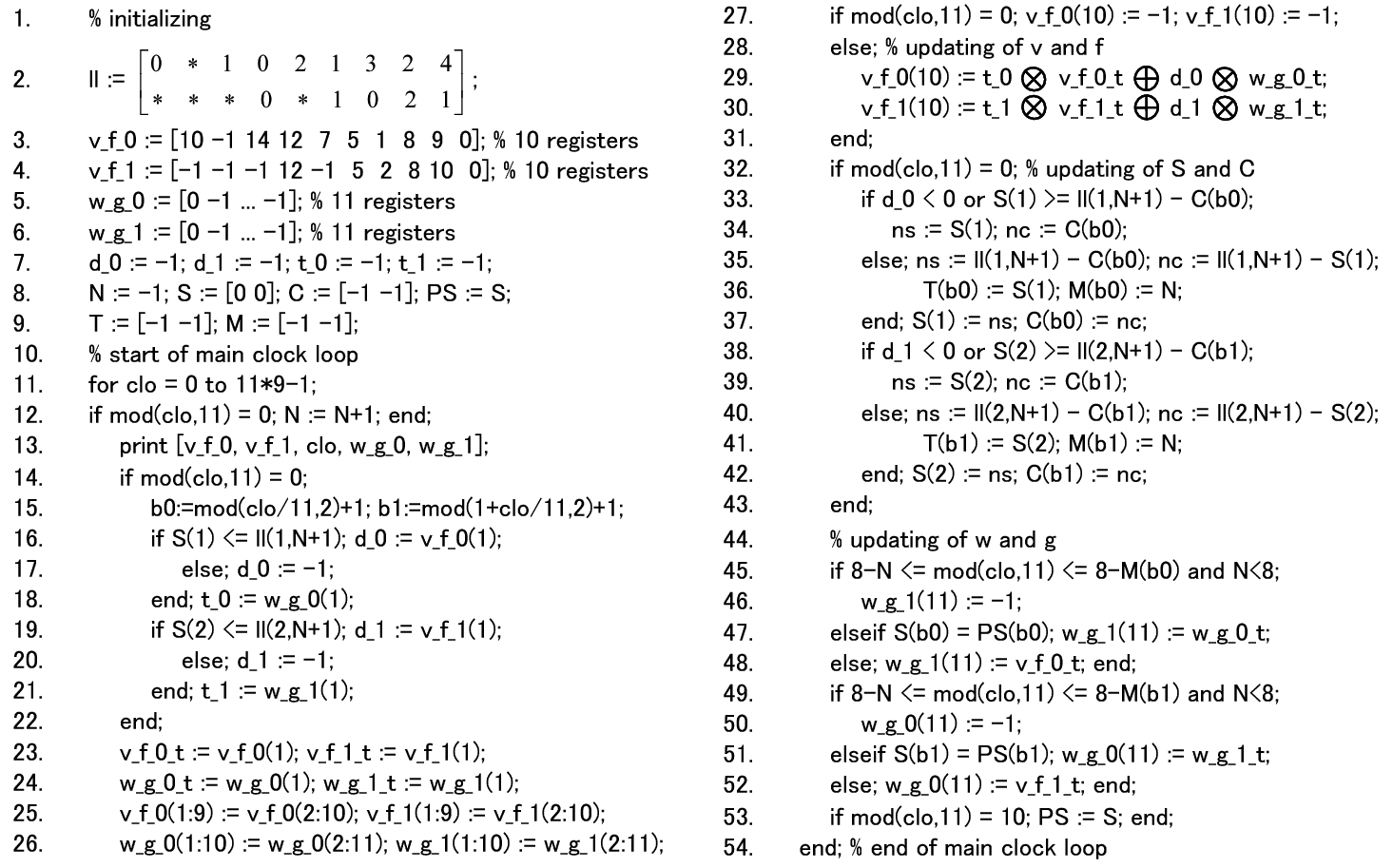
In Fig. 4, we provide a brief description of MATLAB m-file program for our architecture, where returns the smallest non-negative integer satisfying . Comments are written next to “%.” At line 2, ll, which corresponds to the -th component of matrix ll in MATLAB m-file notations, defines with of to decode errors in with . In the case in ll, the logical sentences at lines 16 and 19 are regarded to be false.
In the case of elliptic codes , the number of registers for and should be by (6), and that for and should be , as in lines 3–6 for . At line 15, the value b0 (resp. b1) corresponds to at for (resp. ). At lines 25 and 26, the shift-register values are shifted to the neighbors, and, e.g., “v f 0(1:9):=v f 0(2:10)” indicates the shifts of nine values v f 0(1):=v f 0(2), , v f 0(9):=v f 0(10), where v f 0 corresponds to the -th component of v f 0.
Table II shows that our architecture outputs the
error-locator polynomials and the auxiliary
polynomials for . The top of Table
II indicates the indexes of registers of four
shift-register sequences. The center column indicates the values of “clo” in the program, which corresponds to the underlying clock of the
architecture.
The values of discrepancy are indicated at the left bottom of
Table II, where
“
![[Uncaptioned image]](0705.0286v1/Fig_shaded.png) ’’ indicates
the state that does not exist or .
The values of discrepancy are obtained at clo
from v f 0(1) or v
f 1(1) if .
The values of are indicated at the right bottom of Table
II.
’’ indicates
the state that does not exist or .
The values of discrepancy are obtained at clo
from v f 0(1) or v
f 1(1) if .
The values of are indicated at the right bottom of Table
II.

The most difficult point in the program is that suitable register values must be settled to at the lines 45 and 49 for not changing the coefficients of . Let and be the value of at which the last updating of occurred; we have with at , and have T, M in the program. Then, we claim that , that is, the head coefficient of
is located at the -th register of w g 0 or w g 1 according to or if mod(clo,11) . For example, if clo and N , we can see from in Table II that . Then is in w g 0(6). As another example, if clo and N , we can see that , and then is in w g 0(4).
Noting that the value in w g 0(j) at mod(clo,11) is the shifted value at mod(clo,11) , e.g., w g 0(11) := w g 1(1), we obtain the upper and lower conditions of w g 0(11) and w g 1(11) at lines 45 and 49, since each value of w g 0(j) and w g 1(j) for , , , must be at mod(clo,11) in each . The condition “N8” is required to obtain the values of for error-evaluation (stated below).
Thus, the Gröbner basis of ideal has been obtained together with the auxiliary polynomials . We obtain the set of error-locations through the Chien search, and obtain each error-value by O’Sullivan’s formula [24]
| (20) |
where is the formal derivative of with respect to , e.g., . Note that the divisions in this formula are independent from BMS algorithm, and are calculated by the repetitional multiplications using the multipliers in our architecture as follows.
Since we have for , and have for the sequence defined by and , we see that the calculation of consists of multiplications of and squares, and the total is multiplications in . Thus we can say that our architecture eliminates inverse-calculators, each of which corresponds to multipliers, with slight drop of error-correction capability for .
V Serial architecture
As the second architecture, we describe serial architecture [13], which has a different structure from Kötter’s and the preceding ones. In this section, we focus on well-known codes on Klein’s quartic curve over , and simulate a decoder for it. Many articles so far have treated codes on this curve as examples.
Klein’s quartic curve is defined by equation in projective plane , which causes by in the affine form, and has the same number of -rational points as Hasse–Weil–Serre upper bound 24 with genus 3. We denote -rational points and as and , and other 22 points as the values of . Although it is not a C curve, the monomial basis of to make is obtained by with and the minimal pole order as in Fig. 2. We note that and , and then obtain code of length 23.
We intend to correct generic errors in with (cf. IV-B). Let a primitive element of be . We represent each non-zero element of as the number of powers of as in IV-C. Let the set of error-locations , and let error-values be 1, 2, 5, 4, respectively.
As in the model Fig. 5, the serial architecture has a single structure similar to that of RS codes, while Kötter’s and the preceding inverse-free architectures have an -multiple structure. The initial () arrangement of the coefficients in polynomials is also indicated in Fig. 5. In the case of the architecture for codes on Klein’s quartic, it is convenient to exchange and in all updating formulae (Step 2)–(Step 2), and the validity follows from . For the serial architecture, we employ not the inverse-free BMS algorithm but the original parallel BMS algorithm [16][27], which is described by exchanging updating formulae (11)–(Step 2) into the following (quoted from [16]):
| (21) | ||||
| (24) | ||||
Then the coefficients of and are arranged serially in the order in one sequence of shift-registers, and those of and are arranged in the order in another. This arrangement of coefficients is decided by the pair , and is special to the codes on Klein’s quartic; for codes on C curves, see the next subsection.
Instead of the round of among blocks in the preceding architecture, the order of at is changed to at , and to at , and so on. Although one may change the order of the coefficients of , our layout is easier because of the existence of updating (i.e., the switch “U” in Fig. 5).
![[Uncaptioned image]](0705.0286v1/Table_registervalueS.png)
The exchange register has this role of changing the order. We introduce a method to carry it out with only shift-registers and switches. The following is a small example; at , the switch is down to take the leftmost value in the exchange register, and at other clo’s, the switch is up in order to pass it.
![[Uncaptioned image]](0705.0286v1/Fig_exchange.png)
|
We can see that the exchange register works like a shift-register, since the order-changing has been finished at and the omission by in (14) has been done after more clo’s.
The number of registers in one shift-register sequence for s and s should be equal to the total number of coefficients minus one, i.e., for , and this works like together with the exchange registers. On the other hand, s and s require more shift-registers than s and s because of the structure of parallel BMS algorithm. Thus the number of registers for s and s should be . Then and registers are required for with .
In Fig. 6, we describe the architecture with a MATLAB m-file program, where the notations are the same as in Fig. 4. At line 6, the values of and are initialized differently from all 0 and because of the exclusion of from .
The most difficult point in the program is again that suitable register values should be settled to zero at line 40 in the successive loop for not meeting the coefficients of . Since is at the 49-th register in the initial values of v f r, we claim that (the head coefficient of ) is located at the -th register of w g r if mod(clo,54) . For example, if clo and , we can see from in Table III that . Then are in w g r(16) at clo and 649.
Similarly as in Subsection IV-C, we note that the value in w g r(j) at mod(clo,54) is the shifted value at mod(clo,54) , e.g., w g r(54) := v f r(1). Moreover, since each value of w g r(j) for , , , must be at mod(clo,54) in each , we obtain the upper and lower conditions of w g r(54) at line 40 as the union of


Thus we have obtained the error-locator polynomials
whose common zeros in the rational points decide , and the auxiliary polynomials
Then we obtain each error-value by O’Sullivan’s formula [24]
where is the formal derivative of with respect to , e.g., . The divisions in (20) are not required in this architecture since and have been normalized as .
The definite difference from the preceding one is that the serial architecture has a compact structure analogous to the RS-code case, with one inverse-calculator for the parallel BMS algorithm (not inverse-free). In the next section, we will try to remove it from the serial architecture.
VI Serial inverse-free architecture
We describe serial inverse-free architecture [17], which has the smallest circuit-scale we have ever obtained and is the last among the three kinds of proposed architectures. In this section, we focus on Hermitian codes, that is, codes on Hermitian curves. These codes over have the outstanding properties, and are ones of the most promising candidates for practical use. For simplicity, here we simulate the architecture for a Hermitian code over . The Hermitian curve defined by equation is one of C curves, and has 65 -rational points equal to the Hasse–Weil upper bound with genus . Then codes on this curve can have code-length 64.
![[Uncaptioned image]](0705.0286v1/Table_registervalueSIF.png)
As in the preceding two sections, we intend to correct generic errors in with . The notations concerning are the same as in subsection IV-C. We demonstrate 5-error correction, and set the error-locations , and let error values be 11, 13, 2, 12, 9, respectively.
As shown in the model Fig. 7, the serial inverse-free architecture also has the same single structure as that of RS codes. Initially, the coefficients of s and s are arranged serially in the order in a sequence of shift-registers, and those of s and s are arranged in the order in another. This arrangement of coefficients is decided by the pair with , and in general for other codes on C curves, one can also arrange them in a similar manner with . Then the exchange register changes the order of s at into at , , at . In general, for other codes on C curves, it changes the order of so as to keep as the definition of .
In the case of the serial inverse-free architecture, we require two other sequences of shift-registers, supplementary registers, as in Fig. 7. These do not appear in the algorithm but are due to technical reasons in the architecture. For example, we can see in Table IV that the values and are increased to 3 and 2 at the same . For such cases, the supplementary registers hold the values of the head coefficients and ; otherwise the value cannot be updated to .

For the same reason as the previous ones, suitable register values should be set to zero at line 41, where the condition is derived by taking the supplementary registers into account as follows: Since is at the 101-th register in the initial values of v f r as seen in line 3, we claim that the head coefficient is located at the -th register of w g r if mod(clo,112) . For example, if , we can see from in Table IV that . Then, in w g r(33), is at clo , and is at clo .
Similarly as in section V, we note that the value in w g r(j) at mod(clo,112) is the shifted value at mod(clo,112) , where “” is caused by the supplementary four shift-registers. Moreover, since each value of w g r(j) for , , , must be at mod(clo,112) in each , we obtain the upper and lower conditions of w g r(108) at line 41 as the union of
Thus, the Gröbner basis of ideal and the auxiliary polynomials have been obtained as in Fig. 9, e.g.,
and obtain each error-value by O’Sullivan’s formula (20).
In this manner, we have constructed the smallest-scale architecture, which uses the supplementary registers differently from the others. In our example, the total number of shift-registers for polynomials is 215, while for the supplementary registers, it is 8, i.e., 3.7%. Furthermore, this percentage is decreased for larger , and approximately , as seen in the next section; we have, e.g., for the other Hermitian codes over . Hence we can say that shift-registers for the supplementary registers are reasonably small in the whole architecture.
VII Performance estimation
In this section, we estimate the numbers of multipliers, calculators for inverse, and registers, and the total running time. Although the estimation at Section IX in [16] was done with respect to the upper bound of s, it is now convenient to estimate with respect to of the code since we consider architectures without the determination of unknown-syndrome values.
We quote the result of the systolic array in [16]; the numbers of multipliers and calculators for inverse are and , respectively, as seen at the upper part of Fig.4 in [p.3866,References]. The number of registers and the total running time are and , respectively.
The Kötter’s architecture [7] has multipliers, calculators for inverse, and registers, where since we restrict correctable errors to the generic errors. The total running time takes .
The serial architecture and the serial inverse-free architecture have two multipliers, and the inverse-free architecture has times two multipliers. There is one calculator for inverse only in the serial architecture. The number of registers for these three architectures is equal to times , which consists of the number of syndromes including the gaps plus one for the initial value of ; we ignore the contribution of the discrepancy, exchange, and supplementary registers since these are at most a few multiples of and disappear in the order of . The total running time for the inverse-free architecture agrees with times the number of registers in the sequence for and , which is equal to . Those for the other two agree with .
We summarize these results in Table V, where we denote only the terms of the highest orders for in the estimations. In addition, there is an architecture between Kötter’s and Inverse-free that employs the parallel BMS algorithm (not inverse-free); we call this temporarily parallel-BMS architecture and add it to the table. For example, in the case of Hermitian codes over -element finite field, and is equal to 16 and , respectively. Since the numbers of registers in all architectures have an unchanged order in Table V, we can see that these architectures have optimized their space complexity.
Then we can see in Table V that multipliers have been reduced from Kötter’s to Parallel-BMS, and that inverse-calculators have been reduced from Parallel-BMS to Inverse-free. Both contribute to the reduction of computational complexity. It is noticed that the latter reduction has been accompanied in by the slight decrease of correctable errors that is assignable to error-detection. On the other hand, two types of serial architectures have the constant numbers of finite-field calculators, and their running time takes times longer than that of non-serial types. Thus our serializing method has provided a preferred trade-off between calculators and delay.
![[Uncaptioned image]](0705.0286v1/Table_performance.png)
VIII Conclusions
In this paper, we have proposed the inverse-free parallel BMS algorithm for error-location in decoding algebraic-geometric codes. Thus we have improved decoding bound in [6] based on linear system without the determination of unknown syndromes for AG codes, to for generic errors, where, e.g., and for Hermitian codes over . Moreover, we have constructed three kinds of error-locator architectures using our algorithm. These architectures were not implemented until the determination procedure of unknown syndromes was removed from the error-location algorithm. Our novel algorithm and architectures have a wide range of applications to Gröbner-basis schemes in various algebraic-coding situations, such as Sudan algorithm [29], Guruswami–Sudan algorithm [4], Koetter–Vardy algorithm [8], and encoding of algebraic codes [19].
We have aimed to construct our architectures with only shift-registers, switches, and finite-field calculators. The composition of shift-registers is superior to that of RAMs (random-access memories) in decoding speed, and moreover, our approach is useful for revealing their regularity.
We can conclude that the error-locator architectures correcting generic errors have been completed by the whole from systolic array (max. parallelism) to serial inverse-free ones (min. parallelism). These architectures enable us to fit the decoder of the codes to various sizes and speeds in many applications. It may also be concluded that our methodology, which is the direct decoding from only the received syndromes, correctly generalizes the RS-code case.
Appendix A Proof that is an ideal
We first note that, by (5) and the following lemma,
| (27) |
Lemma 1
We have .
Proof. Obviously equals
where the last equality follows from correspondence .
For simplicity, we denote and as and the error-value without loss of generality. Then we convert the sum in (27) as
| (28) |
Proposition 1
For all , the set is a polynomial ideal.
Proof. Suppose that and with and . Then we show that and . Note that, by (28),
and the last two sums are zero from the assumption and , by Lemma 1. For , note that
and by Lemma 1. Although in general, the monomial is represented as the linear combination of elements in . Then we obtain from the assumption, which completes the proof.
Appendix B Proof of
This follows from the next Corollary and Lemma 2.
Proposition 2
Let be satisfying
and . Then holds.
Proof. Since is converted as (28).
Using Riemann–Roch Theorem, we see that the map
is surjective. Hence there are linearly independent vectors of the form for , and we obtain the following sufficient condition for all errors.
Corollary
Let be satisfying for all . Then holds.
Lemma 2
We can choose a Gröbner basis of as for all .
Proof. First, we notice that an element of Gröbner basis may be determined uniquely by
| (29) |
Let be one of satisfying . We temporarily denote as , where for a divisor . Since we have
where , there is satisfying . Then is obtained by (29), and leads Lemma 2.
Proposition 3
Proof. If and , then is converted similarly as (28) to
Hence, if , then we have , and thus is obvious. To prove , let be a Gröbner basis of , where “” is for consistency in the previous notation. Since , we can choose it as from Lemma 2 and its proof. Now we suppose that for all with . Then we have, by Lemma 1, . Thus we see that the inverse inclusion follows from Corollary Corollary of Proposition 2.
Appendix C Generic case
Let ; recall that is equal to the number of . If , then we have since and . However, for , we have for example for Hermitian curve over . We define that -error position is generic if for and . If is generic, we obtain a Gröbner basis of by solving
with . Then Lemma 2 is improved to for generic .
Conversely, if , then the equation from the linear dependency gives with . Thus we see that is generic if and only if the delta set (footprint in [12]) agrees with . Namely, our definition of generic is equivalent to the definition of generic in [23] and that of “independent” in [5].
Proposition 4
Suppose that is generic.
If , then we have .
In particular, with .
Appendix D Proof of Theorem 1
Theorem 1 is proved by the following three lemmas.
Lemma 3
Suppose that , , and with , , and . Moreover, suppose that and with . Then, at least one condition of and holds.
Proof. We suppose that and . Since and , we have
Since and for , we have and for , and moreover,
where the last equality follows from and for since and for , and the last sum agrees with since and . This contradicts .
Lemma 4
We have .
Proof. We prove it by induction. The case of follows from the initializing. Assuming for all , we prove . We may assume that there is . It follows that . Thus we may assume that , , and without loss of generality. If , then it contradicts Lemma 3 since , , , and . Thus, we obtain and .
Lemma 5
Let , with for , and let , with for . Suppose that , and . Then we have
and , where if , and otherwise.
Proof. Since and
| (30) | ||||
we obtain . Next, since and , we have
We may assume that . If and , then we have and from , and moreover,
Proof of Theorem 1. If and , then and . Thus and hold. Supposing that , let be satisfying , , and , then we have . Thus the theorem except for (17) and (1) follows from Lemma 5. We prove (1) by induction. The case of in (1) holds by the definition. Supposing that the equality is true for , we prove it for . Let be the minimum of in (1). If (P), then , thus holds. If and , then we have as in the proof of Lemma 4 and , which is actually the equation by Lemma 3 for and satisfying . Finally, as for (17), if we suppose with , then we have and , which contradict the minimality of .
Thus we have proved the theorem for an algorithm that is not a parallel version, i.e., the algorithm with direct calculation of by (5) without and . To prove our parallel inverse-free BMS algorithm described in Section III, we have to show further that is obtained by the coefficient of ; we omit this procedure and refer to similar cases [14][16] of ordinary parallel BMS algorithm.
References
- [1] E. R. Berlekamp, Algebraic coding theory, McGraw-Hill, New York, 1968.
- [2] D. Cox, J. Little, D. O’Shea, Ideals, varieties, and algorithms, UTM Springer–Verlag, 1992.
- [3] G.-L. Feng, T. R. N. Rao, “Decoding algebraic-geometric codes up to the designed minimum distance,” IEEE Trans. Inf. Theory, vol.39, pp. 37–45, Jan. 1993.
- [4]
V. Guruswami, M. Sudan,
“Improved decoding of Reed–Solomon and algebraic-geometric codes,”
IEEE Trans. Inf. Theory, vol.45, no.6,
pp.1757–1767, Sep. 1999. - [5] H. E. Jensen, R. R. Nielsen, T. Høholdt, “Performance analysis of a decoding algorithm for algebraic-geometry codes,” IEEE Trans. Inf. Theory, vol.45, no.5, pp.1712–1717, July 1999.
- [6] J. Justesen, K. J. Larsen, H. E. Jensen, A. Havemose, T. Høholdt, “Construction and decoding of a class of algebraic geometry codes,” IEEE Trans. Inf. Theory, vol.35, no.4, pp.811–821, July 1989.
- [7] R. Kötter, “A fast parallel implementation of a Berlekamp–Massey algorithm for algebraic-geometric codes,” IEEE Trans. Inf. Theory, vol.44, no.4, pp.1353–1368, July 1998.
- [8] R. Koetter, A. Vardy, “Algebraic soft-decision decoding of Reed–Solomon codes,” IEEE Trans. Inf. Theory, vol.49, no.11, pp.2809–2825, Nov. 2003.
- [9] K. Lee, M. E. O’Sullivan, “An interpolation algorithm using Gröbner bases for soft-decision decoding of Reed–Solomon codes,” Proc. IEEE Int. Symp. Information Theory, Seattle, July 2006.
- [10] K. Lee, M. E. O’Sullivan, “Sudan’s list decoding of Reed–Solomon codes from a Gröbner basis perspective,” arXiv:math.AC/0601022.
- [11] J. L. Massey, “Shift-register synthesis and BCH decoding,” IEEE Trans. Inf. Theory, vol.IT-15, pp.122–127, Jan. 1969.
- [12] H. Matsui, S. Mita, “Footprint of polynomial ideal and its application to decoder for algebraic-geometric codes,” Proc. Int. Symp. Information Theory and Its Applications (ISITA), pp.1473–1478, Parma, Italy, Oct. 2004.
- [13] H. Matsui, E. Yamamoto, S. Mita, “Reduction of decoder for codes on algebraic curves as an application of footprint,” (in Japanese) Proc. 27th Symp. Information Theory and Its Applications (SITA), pp.471–474, Dec. 2004.
- [14] H. Matsui, S. Sakata, M. Kurihara, “Fast parallel decoding on systolic array architecture for codes on a class of algebraic curves,” RIMS Kokyuroku (Lecture note at Research Institute for Mathematical Sciences in Kyoto University), vol.1420Cpp.193–205, April 2005.
- [15] H. Matsui, S. Mita, “On small-scale decoders for codes on curves,” Proc. Hawaii, IEICE and SITA Joint Conference on Information Theory, IT2005-16, pp.91–95, May 2005.
- [16] H. Matsui, S. Sakata, M. Kurihara, S. Mita, “Systolic array architecture implementing Berlekamp–Massey–Sakata algorithm for decoding codes on a class of algebraic curves,” IEEE Trans. Inf. Theory, vol.51, no.11, pp.3856–3871, Nov. 2005.
- [17] H. Matsui, “On the smallest-scale decoder for codes on algebraic curves,” Proc. 28th Symp. Information Theory and Its Applications (SITA), pp.547–550, Nov. 2005.
- [18]
H. Matsui, S. Mita, “Inverse-free implementation of
Berlekamp–Massey–Sakata algorithm for decoding codes on algebraic curves,” Proc. IEEE Int. Symp. Information Theory, pp.2250–2254, Seattle, July 2006. - [19] H. Matsui, S. Mita, “Efficient encoding via Gröbner bases and discrete Fourier transforms for several kinds of algebraic codes,” Submitted in 2007 IEEE Int. Symp. Information Theory, arXiv:cs.IT/0703104.
- [20] R. Matsumoto, “The curve—A generalization of the Weierstrass form to arbitrary plane curves,” in his website.
- [21]
S. Miura,
“Algebraic geometric codes on certain plane curves,”
(Japanese) Trans. IEICE, J75–A, no.11, pp.1735–1745, Nov. 1992. - [22] Y. Numakami, M. Fujisawa, S. Sakata, “A fast interpolation algorithm for list decoding of Reed–Solomon codes,” (Japanese) Trans. IEICE, vol.J83–A, no.11, pp.1309–1317, Nov. 2000.
- [23] M. E. O’Sullivan, “Decoding Hermitian codes beyond ,” Proc. IEEE International Symposium on Information Theory, p.384, Ulm, Germany, June 29–July 4, 1997. See also “Decoding of Hermitian codes: Beyond the minimum distance bound,” in his website.
- [24] M. E. O’Sullivan, “On Koetter’s algorithm and the computation of error values,” Designs, Codes and Cryptography, vol.31, pp.169–188, 2004.
- [25] S. Sakata, “Finding a minimal set of linear recurring relations capable of generating a given finite two dimensional array,” Journal of Symbolic Computation, no.5, pp.321–337, Nov. 1988.
- [26] S. Sakata, H. E. Jensen, T. Høholdt, “Generalized Berlekamp–Massey decoding of algebraic geometric code up to half the Feng–Rao bound,” IEEE Trans. Inf. Theory, vol.41, no.6, Part I, pp.1762–1768, Nov. 1995.
- [27] S. Sakata, M. Kurihara, “A systolic array architecture for fast decoding of one-point AG codes and scheduling of parallel processing on it,” Proc. AAECC–13 (Eds., M. Fossorier, H. Imai, S. Lin, A. Poli), Lecture Notes in Computer Science, vol.1719, pp.302–313, Springer Verlag, 1999.
- [28] S. Sakata, “Applications of the BMS algorithm to decoding of algebraic codes,” preprint for Workshop on Gröbner bases in Cryptography, Coding Theory and Algebraic Combinatorics, Linz, April 30–May 5, 2006.
- [29] M. Sudan, “Decoding of Reed–Solomon codes beyond the error-correction bound,” Journal of Complexity, vol.13, no.1, pp.180–193, 1997.
- [30] Y. Sugiyama, M. Kasahara, S. Hirasawa, T. Namekawa, “A method for solving key equation for decoding Goppa codes,” Information and Control, vol.27, pp.87–99, 1975.