More Efficient Algorithms and Analyses for Unequal Letter Cost Prefix-Free Coding

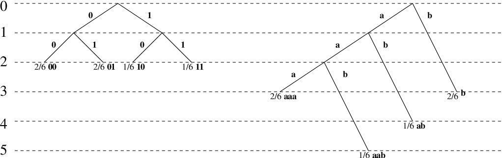
Let $\Sigma=\{\sigma_{1},\sigma_{2}.\ldots,\sigma_{t}\}$ be an encoding alphabet. Word $w\in\Sigma^{*}$ is a prefix of word $w^{\prime}\in\Sigma^{*}$ if $w^{\prime}=wu$ where $u\in\Sigma^{*}$ is a non-empty word. A Code over $\Sigma$ is a collection of words $C=\{w_{1},\ldots,w_{n}\}$. Code $C$ is prefix-free if for all $i\not=j$ $w_{i}$ is not a prefix of $w_{j}.$ See Figure 1.

Let $cost(w)$ be the length or number of characters in $w.$ Given a set of associated probabilities $p_{1},p_{2},\ldots,p_{n}\geq 0$, $\sum_{i}p_{i}=1,$ the cost of the code is $Cost(C)=\sum_{i=1}^{n}cost(w_{i})p_{i}$. The prefix coding problem, sometimes known as the Huffman encoding problem is to find a prefix-free code over $\Sigma$ of minimum cost. This problem is very well studied and has a well-known $O(tn\log n)$-time greedy-algorithm due to Huffman [14] ($O(tn)$-time if the $p_{i}$ are sorted in non-decreasing order).

Alphabetic coding is the same problem with the additional constraint that the codewords must be chosen in increasing alphabetic order (with respect to the words to be encoded). This corresponds, for example, to the problem of constructing optimal (with respect to average search time) search trees for items with the given access probabilities or frequencies. Such a code can be constructed in $O(tn^{3})$ time [16].

One well studied generalization of the problem is to let the encoding letters have different costs. That is, let $\sigma_{i}\in\Sigma$ have associated cost $c_{i}.$ The cost of codeword $w=\sigma_{i_{1}}\sigma_{i_{2}}\ldots\sigma_{i_{l}}$ will be $cost(w)=\sum_{k=1}^{l}c_{i_{k}}$, i.e., the sum of the costs of its letters (rather than the length of the codeword) with the cost of the code still being defined as $Cost(C)=\sum_{i=1}^{n}cost(w_{i})p_{i}$ with this new cost function.

The existing, large, literature on the problem of finding a minimal-cost prefix free code when the $c_{i}$ are no longer equal, which will be surveyed below, assumes that $\Sigma$ is a finite alphabet, i.e., that $t=|\Sigma|<\infty$. The original motivation of this paper was to address the problem when $\Sigma$ is unbounded. which, as will briefly be described in Section 3 models certain types of language restrictions on prefix free codes and the imposition of different cost metrics on search trees. The tools developed, though, turn out to provide improved approximation bounds for many of the finite cases as well. More specifically, it was known [20, 23]¹¹ 1 Note that if $t=2$ with $c_{1}=c_{2}=1$ then $c=1$ and this reduces to the standard entropy lower bound for prefix-free coding. Although the general lower bound is usually only explicitly derived for finite $t$, Krause [20] showed how to extend it to infinite $t$ in cases where a positive root of $1=\sum_{i=1}^{\infty}2^{-cc_{i}}$ exists. that $\frac{1}{c}H(p_{1},\ldots,p_{n})\leq OPT$ where $H(p_{1},\ldots,p_{n})=-\sum_{i=1}^{n}p_{i}\log p_{i}$ is the entropy of the distribution, $c$ is the unique positive root of the characteristic equation $1=\sum_{i=1}^{t}2^{-cc_{i}}$ and $OPT$ is the minimum cost of any prefix free code for those $p_{i}.$ Note that in this paper, $\log x$ will always denote $\log_{2}x.$

The known efficient algorithms create a code $T$ that satisfies

where $C(T)$ is the cost of code $T$, ${{\cal C}}=(c_{1},c_{2},\cdots,c_{t})$ and $f({\cal C})$ is some function of the letter costs ${\cal C}$, with the actual value of $f({\cal C})$ depending upon the particular algorithm. Since $\frac{1}{c}H(p_{1},\ldots,p_{n})\leq OPT$, code $T$ has an additive error at most $f({\cal C})$ from $OPT.$ The $f({\cal C})$ corresponding to the different algorithms shared an almost linear dependence upon the value $c_{t}=\max({\cal C}),$ the largest letter cost. They therefore can not be used for infinite ${\cal C}.$ In this paper we present a new algorithmic variation (all algorithms for this problem start with the same splitting procedure so they are all, in some sense, variations of each other) with a new analysis:

• •

  (Theorems 2 and 3) For finite ${\cal C}$ we derive new additive error bounds $f({\cal C})$ which in many cases, are much better than the old ones.

• •

  (Lemma 9) If ${\cal C}$ is infinite but $d_{j}=|\{m\mid j\leq c_{m}<j+1\}|$ is bounded, then we can still give a bound of type (1). For example, if $c_{m}=1+\lfloor\frac{m-1}{2}\rfloor$, i.e., exactly two letters each of length $i,=1,2,3,\ldots$, then we can show that $f({\cal C})\leq 1+\frac{3}{\log 3}$.

• •

  (Theorem 4) If ${\cal C}$ is infinite but $d_{i}$ is unbounded then we can not provide a bound of type (1) but, as long as $\sum_{i=1}^{\infty}c_{m}2^{-cc_{m}}<\infty$, we can show that

  $$\forall\epsilon>0,\quad C(T)\leq(1+\epsilon)\frac{1}{c}H(p_{1},\ldots,p_{n})+f({\cal C},\epsilon)$$

  (2)

  where $f({\cal C},\epsilon)$ is some constant based only on ${\cal C}$ and $\epsilon$.

We now provide some more history and motivation.

For a simple example, refer to Figure 2. Both codes have minimum cost for the frequencies $(p_{1},p_{2},p_{3},p_{4})=\left(\frac{1}{3},\frac{1}{3},\frac{1}{6},\frac{1}{6}\right)$ but under different letter costs. The code $\{00,01,10,11\}$ has minimum cost for the standard Huffman problem in which of $\Sigma=\{0,1\}$ and $c_{1}=c_{2}=1$, i.e., the cost of a word is the number of bits it contains. The code $\{aaa,aab,ab,b\}$ has minimum cost for the alphabet $\Sigma=\{a,b\}$ in which the length of an “$a$” is 1 and the length of a “$b$” is 3, i.e., ${{\cal C}}=(1,3).$

The unequal letter cost coding problem was originally motivated by coding problems in which different characters have different transmission times or storage costs [4, 22, 18, 27, 28]. One example is the telegraph channel [9, 10, 20] in which $\Sigma=\{\cdot,-\}$ and $c_{1}=1,c_{2}=2$, i.e., in which dashes are twice as long as dots. Another is the $(a,b)$ run-length-limited codes used in magnetic and optical storage [15, 11], in which the codewords are binary and constrained so that each 1 must be preceded by at least $a$, and at most $b$, 0’s. (This example can be modeled by the unequal-cost letter problem by using an encoding alphabet of $r=b-a+1$ characters $\{0^{k}1:k=a,a+1,\ldots,b\}$ with associated costs $\{c_{i}=a+i-1\}$.)

The unequal letter cost alphabetic coding problem arises in designing testing procedures in which the time required by a test depends upon the outcome of the test [19, 6.2.2, ex. 33] and has also been studied under the names dichotomous search [13] or the leaky shower problem [17].

The literature contains many algorithms for the unequal-cost coding problem. Blachman [4], Marcus [22], and (much later) Gilbert [10] give heuristic constructions without analyses of the costs of the codes they produced. Karp gave the first algorithm yielding an exact solution (assuming the letter costs are integers); Karp’s algorithm transforms the problem into an integer program and does not run in polynomial time [18]. Later exact algorithms based on dynamic programming were given by Golin and Rote [11] for arbitrary $t$ and a slightly more efficient one by Bradford et. al. [5] for $t=2.$. These algorithms run in $n^{\theta(c_{t})}$ time where $c_{t}$ is the cost of the largest letter. Despite the extensive literature, there is no known polynomial-time algorithm for the generalized problem, nor is the problem known to be NP-hard. Golin, Kenyon and Young [12] provide a polynomial time approximation scheme (PTAS). Their algorithm is mainly theoretical and not useful in practice. Finally, in contrast to the non-alphabetic case, alphabetic coding has a polynomial-time algorithm $O(tn^{3})$ time algorithm [16].

Karp’s result was followed by many efficient algorithms [20, 8, 7, 23, 2]. As mentioned above, $\frac{1}{c}H(p_{1},\ldots,p_{n})\leq OPT$; almost²² 2 As mentioned by Mehlhorn [23], the result of Cot [7] is a bit different. It’s a redundancy bound and not clear how to efficiently implement as an algorithm. Also, the redundancy bound is in a very different form involving taking the ratio of roots of multiple equations that makes it difficult to compare to the others in the literature. all of these algorithms produce codes of cost at most $C(T)\leq\frac{1}{c}H(p_{1},\ldots,p_{n})+f({\cal C})$ and therefore give solutions within an additive error of optimal. An important observation is that the additive error in these papers $f({{\cal C}})$ somehow incorporate the cost of the largest letter $c_{t}=\max({\cal C})$. Typical in this regard is Mehlhorn’s algorithm [23] which provides a bound of

Thus, none of the algorithms described can be used to address infinite alphabets with unbounded letter costs.

The algorithms all work by starting with the probabilities in some given order, grouping consecutive probabilities together according to some rule, assigning the same initial codeword prefix to all of the probabilities in the same group and then recursing. They therefore actually create alphabetic codes. Another unstated assumption in those papers (related to their definition of alphabetic coding) is that the order of the $c_{m}$ is given and must be maintained.

In this paper we are only interested in the general coding problem and not the alphabetic one and will therefore have freedom to dictate the original order in which the $p_{i}$ are given and the ordering of the $c_{m}.$ We will actually always assume that $p_{1}\geq p_{2}\geq p_{2}\geq\cdots$ and $c_{1}\leq c_{2}\leq c_{3}\leq\cdots$. These assumptions are the starting point that will permit us to derive better bounds. Furthermore, for simplicity, we will always assume that $c_{1}=1.$ If not, we can always force this by uniformly scaling all of the $c_{i}.$

For further references on Huffman coding with unequal letter costs, see Abrahams’ survey on source coding [1, Section 2.7], which contains a section on the problem.

There is a very standard correspondence between prefix-free codes over alphabet $\Sigma$ and $|\Sigma|$-ary trees in which the $m^{\mbox{th}}$ child of node $v$ is labelled with character $\sigma_{m}\in\Sigma.$ A path from the root in a tree to a leaf will correspond to the word constructed by reading the edge labels while walking the path. The tree $T$ corresponding to code $C=\{w_{1},\ldots,w_{n}\}$ will be the tree containing the paths corresponding to the respected words. Note that the leaves in the tree will then correspond to codewords while internal nodes will correspond to prefixes of codewords. See Figures 2 and 5.

Because this correspondence is 1-1 we will speak about codes and trees interchangeably, with the cost of a tree being the cost of the associate code.

We note that many of the previous results in the literature, e.g., (3) from [23], were stated in terms of ${\rm NR}.$ We will see later that this is a very natural measure for deriving bounds. Also, note that by the lower bound previously mentioned, $C(T)\geq\frac{1}{c}H(p_{1},\ldots,p_{n})$ for all $T$ and $p_{i}$, so $R(T;p_{1},\ldots,p_{n})$ is a good measure of absolute error.

It is very easy to understand the unequal-cost letter problem as modelling situations in which different characters have different transmission times or storage costs [4, 22, 18, 27, 28]. Such cases will all have finite alphabets. It is not a-priori as clear why infinite alphabets would be interesting. We now discuss some motivation.

In what follows we will need some basic language notation. A language ${\cal L}$ is just a set of words over alphabet $\Sigma.$ The concatenation of languages $A$ and $B$ is $AB=\{ab\mid a\in A,b\in B\}.$ The $i$-fold concatenation, ${\cal L}^{i}$, is defined by ${\cal L}^{0}=\{\lambda\}$ (the language containing just the empty string), ${\cal L}^{1}={\cal L}$ and ${\cal L}^{i}={\cal L}{\cal L}^{i-1}.$ The Kleene star of ${\cal L}$, is ${\cal L}=\bigcup_{i=0}^{\infty}{\cal L}^{i}$.

We start with cost vector ${\cal C}=\{1,2,3,\ldots,\}$ i.e, $\forall m>0,c_{m}=m.$ An early use of this problem was [24]. The idea there was to construct a tree (not a code) in which the internal pointers to children were stored in a linked list. Taking the $m^{\mbox{\small th}}$ pointer corresponds to using character $\sigma_{m}.$ The time that it takes to find the $m^{\mbox{\small th}}$ pointer is proportional to the location of the pointer in the list. Thus (after normalizing time units) $c_{m}=m.$

We now consider a generalization of the problem of 1-ended codes. The problem of finding min-cost prefix free code with the additional restriction that all codewords end with a 1 was studied in [3, 6] with the motivation of designing self-synchronizing codes. One can model this problem as follows. Let ${\cal L}$ be a language. In our problem,

We say that a code $C$ is in ${\cal L}$ if $C\subseteq{\cal L}.$ The problem is to find a minimum cost code among all codes in ${\cal L}.$

Now suppose further that ${\cal L}$ has the special property that ${\cal L}={\cal Q}^{*}$ where ${\cal Q}$ is itself a prefix-free language. Then every word in ${\cal L}$ can be uniquely decomposed as the concatenation of words in ${\cal Q}$. If the decomposition of $w\in{\cal L}$ is $w=q_{1}q_{2}\ldots q_{r}$ for $q_{i}\in{\cal Q}$ then $cost(w)=\sum_{i=1}^{r}cost(q_{i}).$ We can therefore model the problem of finding a minimum cost code among all codes in ${\cal L}$ by first creating an infinite alphabet $\Sigma_{\cal Q}=\{\sigma_{q}\mid q\in Q\}$ with associated cost vector $C_{\cal Q}$ (in which the length of $\sigma_{q}$ is $cost(q)$) and then solving the minimal cost coding problem for $\Sigma_{\cal Q}$ with those associated costs. For the example of 1-ended codes we set ${\cal Q}=\{1,01,001,0001,\ldots\}$ and thus have ${\cal C}=\{1,2,3,\ldots,\}$ i.e, an infinite alphabet with $c_{m}=1$ for all $m\geq 1.$

Now consider generalizing the problem as follows. Suppose we are given an unequal cost coding problem with finite alphabet $\Sigma=\{\sigma_{1},\ldots,\sigma_{t}\}$ and associated cost vector ${\cal C}=(c_{1},\ldots,c_{t}).$ Now let $\Sigma^{\prime}\subset\Sigma$ and define

Now note that ${\cal L}=D^{*}$ where $D=(\Sigma-\Sigma^{\prime})^{*}\Sigma^{\prime}$ is a prefix-free language. We can therefore model the problem of finding a minimum cost code among all codes in ${\cal L}$ by solving an unequal cost coding problem with alphabet $\Sigma_{D}$ and ${\cal C}_{D}.$ The important observation is that

the number of letters in $\Sigma_{D}$ of length $j$, satisfies a linear recurrence relation. Bounding redundancies for these types of ${\cal C}$ will be discussed in Section 6, Case 4.

As an illustration, consider $\Sigma=\{1,2,3\}$ with ${\cal C}=(1,1,2)$ and $\Sigma^{\prime}=\{1\}$; our problem is find minimal cost prefix free codes in which all words end with a $1.$ ${\cal L}=\{1,2,3\}^{*}\{1\}=D^{*}$, where $D=\{2,3\}^{*}\{1\}.$ The number of characters in $\Sigma_{D}$ with length $j$ is

and, in general, $d_{i+2}=d_{i+1}+d_{i}$, so $d_{i}=F_{i},$ the Fibonacci numbers.

We conclude with a very natural ${\cal L}$ for which we do not know how to analyze the redundancy. In Section 6, Case 5 we will discuss why this is difficult.

Let ${\cal L}$ be the set of all ‘‘balanced’’ binary words³³ 3 This also generalizes a problem from [21] which provides heuristics for constructing a min-cost prefix-free code in which the expected number of 0’s equals the expected number of 1’s., i.e., all words which contain exactly as many 0’s as 1’s. Note that ${\cal L}={\cal D}^{*}$ where ${\cal D}$ is the set of all non-empty balanced words $w$ such that no prefix of $w$ is balanced. Let

and set $L(z)=\sum_{n=0}^{\infty}\ell_{n}z^{n}$ and $D(z)=\sum_{n=0}^{\infty}d_{n}z^{n}$ to be their associated generating functions. If ${\cal L}=D^{*}$, then standard generating function rules, see e.g., [25], state that $L(z)=(1-D(z))^{-1}.$ Observe that $l_{n}=0$ if $n$ is odd and $l_{n}={{n}\choose{n/2}}$ for $n$ even, so

and

This can then be solved to see that, for even $n>0$, $d_{n}=2C_{n/2-1}$ where $C_{i}=\frac{1}{i+1}{{2i}\choose i}$ is the $i^{\mbox{\small th}}$ Catalan number. For $n=0$ or odd $n$, $d_{n}=0.$

All of the provably efficient heuristics for the problem, e.g., [20, 8, 7, 23, 2], use the same basic approach, which itself is a generalization of Shannon’s original binary splitting algorithm [26]. The idea is to create $t$ bins, where bin $m$ has weight $2^{-cc_{m}}$ (so the sum of all bin weights is $1$). The algorithms then try to partition the probabilities into the bins; bin $m$ will contain a set of contiguous probabilities $p_{l_{m}},p_{l_{m}+1},\ldots,p_{r_{m}}$ whose sum will have total weight ”close” to $2^{-cc_{m}}.$ The algorithms fix the first letter of all the codewords associated with the $p_{k}$ in bin $m$ to be $\sigma_{m}.$ After fixing the first letter, the algorithms then recurse, normalizing $p_{l_{m}},p_{l_{m}+1},\ldots,p_{r_{m}}$ to sum to $1$, taking them as input and starting anew. The various algorithms differ in how they group the probabilities and how they recurse. See Figures 5, 5 and 5 for an illustration of this generic procedure.

Here we use a generalization of the version introduced in [23]. The algorithm first preprocesses the input and calculates all $P_{k}=p_{1}+p_{2}+\ldots+p_{k}$ ($P_{0}=0$)and $s_{k}=p_{1}+p_{2}+\ldots+p_{k-1}+\frac{p_{k}}{2}$. Note that if we lay out the $p_{i}$ along the unit interval in order, then $s_{k}$ can be seen as the midpoint of interval $p_{i}.$ It then partitions the probabilities into ranges, and for each range it constructs left and right boundaries $L_{m},R_{m}$. $p_{k}$ will be assigned to bin $m$ if it “falls” into the “range” $[L_{m},R_{m})$.

If the interval $p_{k}$ falls into the range, i.e., $L_{m}\leq P_{k-1}<P_{k}<R_{m}$ then $p_{k}$ should definitely be in bin $m$. But what if $p_{k}$ spans two (or more) ranges, e.g., $L_{m}\leq P_{k-1}<R_{m}<P_{k}$? To which bin should $p_{k}$ be assigned? The choice made by [23] is that $p_{k}$ is assigned to bin $m$ if $s_{k}=p_{1}+p_{2}+\ldots+p_{k}/2$ falls into $[L_{m},R_{m})$, i.e., the midpoint of $p_{k}$ falls into the range.

Our procedure $CODE(l,r,U)$ will build a prefix-free code for $p_{l},\ldots,p_{r}$ in which every code word starts with prefix $U$. To build the entire code we call $CODE(1,n,\lambda)$, where $\lambda$ is the empty string.

The procedure works as follows (Figure 6 gives pseudocode and Figures 9, 9 and 9 illustrate the concepts):

Assume that we currently have a prefix of $U$ assigned to $p_{l},\ldots,p_{r}$. Let $v$ be node in the tree associated with $U.$ Let $w(v)=\sum_{k=l}^{r}p_{k}.$

(i) If $l=r$ then word $U$ is assigned to $p_{l}$. Correspondingly, $v$ is a leaf in the tree with weight $w(v)=p_{l}.$

(ii) Otherwise let $L=P_{l}$ and $R=P_{r}$. Split $R-L=w(v)$ into $t$ ranges⁴⁴ 4 In the description, $t$ is permitted to be finite or infinite. as follows.

Insert $p_{k}$, $l\leq k\leq r$ in bin $m$ if $s_{k}\in[L_{m},R_{m})$. Bin $m$ will thus contain the $p_{k}$ in $I^{*}_{m}(v)=\{k\mid L_{m}\leq s_{k}<R_{m}\}$.

We now shift the items $p_{k}$ leftward in the bins as follows. Walk through the bins from left to right. If the current bin already contains some $p_{k}$, continue to the next bin. If the current bin is empty, take the first $p_{k}$ that appears in a bin to the right of the current one, shift $p_{k}$ into the current bin and walk to the next bin. Stop when all $p_{k}$ have been seen. Let $I_{m}(v)$ denote the items in the bins after this shifting.

Note that after performing this shifting there is some $M(v)$ such that all bins $m\leq M(v)$ are nonempty and all bins $m>M(v)$ are empty. Also notice that it is not necessary to actually construct the $I^{*}_{m}(v)$ first. We only did so because they will be useful in our later analysis. We can more efficiently construct the $I_{m}(v)$ from scratch by walking from left to right, using a binary search each time, to find the rightmost item that should be in the current bin. This will take $O(M(v)\log(l-r))$ time in total.

We then check if all of the items are in $I_{1}(v)$. If they are, we take $p_{r}$ and move it into $I_{2}(v)$ (and set $M(v)=2$).

Finally, after creating the all of the $I_{m}(v)$ we let $l_{m}=\min\{k\in I_{m}(v)\}$ and $r_{m}=\max\{k\in I_{m}(v)\}$ and recurse, for each $m<M(v)$ building $CODE(l_{m},r_{m},U\sigma_{m})$

It is clear that the algorithm builds some prefix code with associated tree $T$. As defined, let $N_{T}$ be the set of internal nodes of $T.$ Since every internal node of $T$ has at least two children, $\sum_{v\in N_{T}}M(v)\leq 2n-1.$

The algorithm uses $O(1)$ time at each of its $n$ leaves and $O(M(v)\log n)$ time at node $v.$ Its total running time is thus bounded by

with no dependence upon $t.$

For comparison, we point out the algorithm in [23] also starts by first finding the $I^{*}_{m}(v)$. Since it assumed $t<\infty$, its shifting stage was much simpler, though. It just shifted $p_{l}$ into the first bin and $p_{r}$ into the $t^{\mbox{th}}$ bin (if they were not already there).

We will now see that our modified shifting procedure not only permits a finite algorithm for infinite encoding alphabets, but also often provides a provably better approximation for finite encoding alphabets.

In the analysis we define $w^{*}_{m}(v)=\sum_{k\in I^{*}_{m}(v)}p_{k}$, $w_{m}(v)=\sum_{k\in I_{m}(v)}p_{k}$. Note that $w(v)=\sum_{m=1}^{t}w^{*}_{m}(v)=\sum_{m=1}^{t}w_{m}(v)=\sum_{k=l}^{r}p_{k}$.

We first need three Lemmas from [23]. The first was proven by recursion on the nodes of a tree, the second followed from the definition of the splitting procedure and the third from the second by some algebraic manipulations.

Lemma 1 permits expressing the normalized redundancy of $T$ as

Set

Note that ${\rm NR}(T)=\sum_{v\in N_{T}}w(v)\left(\sum_{m=1}^{t}E(v,m)\right).$ For convenience we will also define

The analysis proceeds by bounding the values of ${\rm NR}^{*}(T)$ and ${\rm NR}(T)-{\rm NR}^{*}(T)$.

References

- [1] Julia Abrahams. Code and parse trees for lossless source encoding. Communications in Information and Systems, 1(2):113–146, April 2001.
- [2] Doris Altenkamp and Kurt Melhorn. Codes: Unequal probabilies, unequal letter costs. Journal of the Association for Computing Machinery, 27(3):412–427, July 1980.
- [3] Toby Berger and Raymond W. Yeung. Optimum ’1’ ended binary prefix codes. IEEE Transactions on Information Theory, 36(6):1435–1441, 1990.
- [4] N. M. Blachman. Minimum cost coding of information. IRE Transactions on Information Theory, PGIT-3:139–149, 1954.
- [5] P. Bradford, M. Golin, L. L. Larmore, and W. Rytter. Optimal prefix-free codes for unequal letter costs and dynamic programming with the monge property. Journal of Algorithms, 42:277–303, 2002.
- [6] Renato M. Capocelli, Alfredo De Santis, and Giuseppe Persiano. Binary prefix codes ending in a ”1”. IEEE Transactions on Information Theory, 40(4):1296–1302, 1994.
- [7] Norbert Cott. Characterization and Design of Optimal Prefix Codes. PhD Thesis, Stanford University, Department of Computer Science, June 1977.
- [8] I. Csisz’ar. Simple proofs of some theorems on noiseless channels. Inform. Contr., 514:285–298, 1969.
- [9] E. N. Gilbert. How good is morse code. Inform Control, 14:585–565, 1969.
- [10] E. N. Gilbert. Coding with digits of unequal costs. IEEE Trans. Inform. Theory, 41:596–600, 1995.
- [11] M. Golin and G. Rote. A dynamic programming algorithm for constructing optimal prefix-free codes for unequal letter costs. IEEE Transactions on Information Theory, 44(5):1770–1781, 1998.
- [12] Mordecai J. Golin, Claire Kenyon, and Neal E. Young. Huffman coding with unequal letter costs. In Proceedings of the 34th Annual ACM Symposium on Theory of Computing (STOC’02), pages 785–791, 2002.
- [13] K. Hinderer. On dichotomous search with direction-dependent costs for a uniformly hidden objec. Optimization, 21(2):215–229, 1990.
- [14] D. A. Huffman. A method for the construction of minimum redundancy codes. In Proc. IRE 40, volume 10, pages 1098–1101, September 1952.
- [15] K. A. S. Immink. Codes for Mass Data Storage Systems. Shannon Foundations Publishers, 1999.
- [16] I. Itai. Optimal alphabetic trees. SIAM J. Computing, 5:9–18, 1976.
- [17] Sanjiv Kapoor and Edward M. Reingold. Optimum lopsided binary trees. Journal of the Association for Computing Machinery, 36(3):573–590, July 1989.
- [18] Richard Karp. Minimum-redundancy coding for the discrete noiseless channel. IRE Transactions on Information Theory, IT-7:27–39, January 1961.
- [19] Donald E. Knuth. The Art of Computer Programming, Volume III: Sorting and Searching. Addison-Wesley, 1973.
- [20] R. M. Krause. Channels which transmit letters of unequal duration. Inform. Contr., 5:13–24, 1962.
- [21] Jia-Yu Lin, Ying Liu, and Ke-Chu Yi. Balance of 0, 1 bits for huffman and reversible variable-length coding. IEEE Transactions on Communications, 52(3):359–361, 2004.
- [22] R.S. Marcus. Discrete Noiseless Coding. M.S. Thesis, MIT E.E. Dept, 1957.
- [23] K. Mehlhorn. An efficient algorithm for constructing nearly optimal prefix codes. IEEE Trans. Inform. Theory, 26:513–517, September 1980.
- [24] Yale N. Patt. Variable length tree structures having minimum average search time. Commun. ACM, 12(2):72–76, 1969.
- [25] Robert Sedgewick and Philippe Flajolet. An introduction to the analysis of algorithms. Addison-Wesley Longman Publishing Co., Inc., Boston, MA, USA, 1996.
- [26] Claude E. Shannon. A mathematical theory of communication. The Bell System Technical Journal, 27:379–423, 623–656, July, October 1948.
- [27] L. E. Stanfel. Tree structures for optimal searching. Journal of the Association for Computing Machinery, 17(3):508–517, July 1970.
- [28] B. Varn. Optimal variable length codes (arbitrary symbol cost and equal code word probability). Information Control, 19:289–301, 1971.