Joint free energy distribution in the random directed polymer problem

Directed polymers subject to a random potential exhibit non-trivial behavior deriving from the interplay between elasticity and disorder; numerous physical systems can be mapped onto this model and the topic has been the subject of intense studies hh_zhang_95. Despite its undisputable importance, our knowledge on this generic problem is still limited. Traditionally, the main focus is on the free energy distribution function, for which two types of analytical solutions are known for the $(1+1)$-dimensional case, a polymer confined to a plane (see Fig. 1): one class addresses the ‘longitudinal’ problem and determines the distribution function ${\cal P}_{L}(F)$ for the free energy $F$ of a polymer of length $L$ and fixed endpoint $y=0$ kardar_87; zhang_89; spohn_00; monthus_04; kk_06, while the other concentrates on the ‘transverse’ problem aiming at the distribution function ${\cal P}_{u}(F^{\prime})$ involving the free energy difference $F^{\prime}=F^{+}\!-\!F^{-}$ between two configurations with endpoints at $y=\pm u$ hhf_85; parisi_90; spohn_02, assuming no dependence on the mean energy $\bar{F}\!=\!(F^{+}\!+\!F^{-})/2$ in the limit $L\!\to\!\infty$. Both approaches have been helpful in finding the wandering exponent $\zeta$ hh_85 of transverse fluctuations $\delta y(L)\propto L^{\zeta}$ of the polymer. On the other hand, questions how the result for ${\cal P}_{u}(F^{\prime})$ is approached from finite $L$ and how the transverse and longitudinal problems are interrelated have remained unclear; it is the purpose of this letter to shed light upon these issues.

Here, we generalize the task of finding the free energy distribution function for a polymer of length $L$ by studying two configurations of the string ending in two points separated by $2u$, see Fig. 1, and treating both the mean free energy $\bar{F}$ and the free energy difference $F^{\prime}$ as relevant variables. The two-point object $F^{\prime}$ relates to the natural variable appearing in the Burgers problem hhf_85, while for $u=0$ the variable $\bar{F}$ reduces to the free energy $F$ of a single configuration studied in Refs. kardar_87; zhang_89; spohn_00; monthus_04; kk_06. Our new scheme then should allow us to place the previous results for ${\cal P}_{L}(F)$ and ${\cal P}_{u}(F^{\prime})$ into a common context. Using the replica approach, we determine the joint distribution function ${\cal P}_{L,u}(\bar{F},F^{\prime})$ and prove (for a $\delta$-correlated disorder potential) the separation ${\cal P}_{L,u}(\bar{F},F^{\prime})={P}_{L,u}(\bar{F})\,{P}_{u}(F^{\prime})$ in the limit of large $L$ and for large negative values of the mean free energy $\bar{F}$. Furthermore, we derive the form of the two factors ${P}_{L,u}(\bar{F})$ and ${P}_{u}(F^{\prime})$: on the one hand, we find that ${P}_{L,u}(\bar{F})$ has the same form as Zhang’s tail zhang_89 for ${\cal P}_{L}(F)$. On the other hand, to our surprise, we find that the transverse part ${P}_{u}(F^{\prime})$ exactly coincides with the stationary distribution function ${\cal P}_{u}(F^{\prime})$ of the Burgers problem hhf_85, although our solution is associated with rare events in the far-left tail, while the result of Ref. hhf_85 describes an equilibrium situation reached in the limit $L\to\infty$. In the following, we first describe the previous replica analysis leading to the distribution function ${\cal P}_{L}(F)$ and its potential pitfalls and then proceed with the derivation of the joint distribution function ${\cal P}_{L,u}(\bar{F},F^{\prime})$.

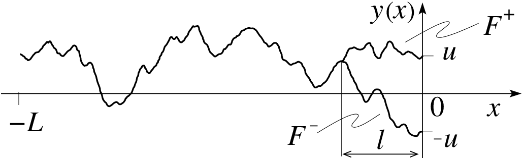
We consider an elastic string (elasticity $c$) directed along the $x$-axis within an interval $[-L,0]$ and subject to a disorder potential $V[x,y]$ driving the displacement field $y(x)$, see Fig. 1; its energy is given by

The disorder average is carried out over a Gaussian distribution with zero mean $\langle V(x,y)\rangle_{\scriptscriptstyle V}=0$ and a $\delta$-correlator $\langle{V(x,y)V(x^{\prime},y^{\prime})}\rangle_{\scriptscriptstyle V}=U_{0}\,\delta(x-x^{\prime})\delta(y-y^{\prime})$.

The standard procedure kardar_87 leading to the distribution function ${\cal P}_{L}(F)$ starts from the partition function (we set the Boltzmann constant $k_{B}$ equal to unity)

providing us with the free energy $F(L;V)=-T{\rm ln}Z$. The $N$-fold replication of the polymer and subsequent averaging over disorder realizations $V$ maps the problem to $N$ quantum bosons with local interactions $-U_{0}\delta(y-y^{\prime})/T$. In the large $L$ limit, the replica partition function $Z_{r}(N;L)=\langle Z^{N}(L;V)\rangle_{\scriptscriptstyle V}$ is dominated by the ground state of the quantum problem, which can be obtained from a Bethe Ansatz solution McGuire_64, $Z_{r}(N;L)\propto\exp[-(N\langle F\rangle_{\scriptscriptstyle V}+e_{3}N^{3}L)/T]$ (with $e_{3}=-cU_{0}^{2}/24T^{4}$). Exploiting the relation between the replica partition function $Z_{r}(N;L)$ and ${\cal P}_{L}(F)$ as given by the bilateral Laplace transform

allows one to show zhang_89 that the far-left tail of the distribution function ${\cal P}_{L}(F)$ assumes the form ${\cal P}_{L}(F)\propto\exp[-(2/3)(|F|/F_{\ast})^{3/2}]$ with the characteristic free energy scale $F_{\ast}=(cU_{0}^{2}L/8T^{2})^{1/3}\propto L^{1/3}$.

In Ref. kardar_87, an attempt has been made to use the result for $Z_{r}(N;L)$ and extract the third moment of the distribution function ${\cal P}_{L}(F)$. While predicting a wrong prefactor krug_92, this approach also misses to produce results for other moments. The reason for this failure was identified by Medina and Kardar Medina_93; Kardar_LH, who pointed out that the two limits $L\to\infty$ (allowing to ignore excited states) and $N\to 0$ (providing the irreducible moments $\langle\langle F^{k}\rangle\rangle_{\scriptscriptstyle V}=(-T)^{k}\partial^{k}_{N}\ln\langle Z_{r}(N;L)|_{N\to 0}$ of the distribution function) do not commute. To obtain estimates for moments, the assumption has to be made that the distribution function ${\cal P}_{L}(F)$ is governed by a unique free energy scale $F_{\ast}\propto L^{1/3}$; although this assumption cannot be expected to work for the very distant (non-equilibrium) tails, it turns out that its validity indeed extends to the far-left tail in the present problem, but does not for the far-right tail kk_06. Summarizing, the original Bethe Ansatz solution kardar_87 allows one to find the (far-left) tail of the distribution function zhang_89 but cannot a priori provide information on its body Medina_93; Kardar_LH; Bouchaud_90 as this requires knowledge of the behavior of $Z_{r}(N;L)$ for $N\to 0$.

Here, we study a different setup involving two configurations of a polymer with length $L$ ending in points separated by $2u$; we define the mean free energy $\bar{F}=(F^{\scriptscriptstyle+}+F^{\scriptscriptstyle-})/2$ and difference $F^{\prime}=F^{\scriptscriptstyle+}-F^{\scriptscriptstyle-}$, with $F^{\scriptscriptstyle\pm}\equiv F(L,\pm u;V)$ the free energies of polymers ending in $y(0)=\pm u$. The quantities $\bar{F}$ and $F^{\prime}$ are random variables and we are aiming for the joint distribution function ${\cal P}_{L,u}(\bar{F},F^{\prime})$. We define the replica partition function $Z_{r}^{\prime}(n,m;L,u)$, which can be expressed as the bilateral Laplace transform of ${\cal P}_{L,u}(\bar{F},F^{\prime})$,

The average over disorder realizations $V$ provides us with the replica partition function in the form

with the replica Hamiltonian

The replica partition function $Z_{r}^{\prime}(n,m;L,u)$ describes a system with $n+m$ trajectories $y_{a}(x)$ ($a=1,\dots,n+m$) of which $n$ traces terminate at the point $u$, while the other $m$ trajectories end in the point $-u$; we adopt free initial conditions notefi at $x=-L$ as implied by the absence of any restriction on $y_{a}(-L)$ in (5). All these trajectories are coupled by the attractive potential $-U_{0}\delta(y_{a}-y_{b})/T$ deriving from the disorder correlator.

We use the standard way kardar_87 to map the path integral (5) to a Schrödinger problem: allowing the $n+m$ trajectories to end in an arbitrary point ${\bf y}=(y_{1},\dots,y_{n+m})$, we define the wave function $\Psi({\bf y};x)=Z_{r}^{\prime}(n,m;L+x,{\bf y})$ which satisfies the imaginary-time Schrödinger equation $-T\partial_{x}\Psi({\bf y};x)=\hat{H}\Psi({\bf y};x)$ with the initial condition $\Psi({\bf y};-L)=1$. The Hamiltonian reads

and describes $n+m$ particles of mass $c/T^{2}$ interacting via the attractive two-body potential $-U_{0}\delta(y-y^{\prime})/T$. The partition function (5) is obtained by a particular choice of the final-point coordinates, $Z_{r}^{\prime}(n,m;L,u)=\Psi({\bf u};0)$ with ${\bf u}\equiv(u_{1},\dots,u_{n}=u;u_{n+1},\dots,u_{n+m}=-u)$.

The expansion of $\Psi\bigl({\bf y};x\bigr)$ in terms of eigenfunctions $\Psi_{K,\alpha}=\exp[iK\sum_{a}y_{a}/(n+m)]\psi_{\alpha}(\{y_{a}\})$ of (7) involves a center of mass component and a factor $\psi_{\alpha}(\{y_{a}\})$ depending only on relative coordinates $y_{a}-y_{b}$. Our choice of free initial condition $\Psi({\bf y};-L)=1$ implies a vanishing center of mass momemtum $K=0$ and our expansion assumes the simplified form

with $E_{\alpha}$ the eigenenergies. The coefficients $c_{\alpha}=\langle\psi_{\alpha}|\Psi(-L)\rangle/\langle\psi_{\alpha}|\psi_{\alpha}\rangle$ follow from the initial condition $\Psi({\bf y};-L)=1$ with the scalar product $\langle\psi|\phi\rangle=\int[\prod_{a}dy_{a}]\,\delta\bigl[\sum_{a}y_{a}/(n+m)\bigr]\psi(\{y_{a}\})\phi(\{y_{a}\})$.

In the limit of large $L$, fixed $u$, and for integer $n,m\geq 1$ (see below for a detailed discussion on limits and scaling $u$ versus $L$) the sum in (8) is dominated by the ground state wave function $\psi_{0}$, for which the Bethe Ansatz provides the solution McGuire_64

with the inverse length $\kappa=cU_{0}/4T^{3}$ and the energy noteE

The normalization $\langle\psi_{0}|\psi_{0}\rangle=(n+m)/(4\kappa)^{n+m-1}\Gamma(n+m)$ and the matrix element $\langle\psi_{0}|\Psi(-L)\rangle=(n+m)/(2\kappa)^{n+m-1}\Gamma(n+m)$ provide the result $\Psi({\bf y};0)=2^{n+m-1}e^{-\beta E_{0}L}\psi_{0}({\bf y})$ and evaluating (9) at the endpoint ${\bf u}$, we obtain the expression $\psi_{0}({\bf u})=\exp[-4\kappa|u|nm]$ and hence

Rewriting the exponent $4\kappa|u|nm=\kappa|u|[(n+m)^{2}+(n-m)^{2}]$, we can factorize $Z_{r}^{\prime}(n,m;L,u)=Z_{r}^{+}(n+m;L,u)$ $Z_{r}^{-}(n-m;u)$ with

depending only on the variables $n+m$ and $n-m$, cf. (4). Hence we find that the ‘transverse’ problem described by $Z_{r}^{-}(n-m;u)$ can be separated from the (mainly) ‘longitudinal’ part encoded in $Z_{r}^{+}(n+m;L,u)$. This separation into transverse and longitudinal factors is a central element of our solution and tells us that the joint distribution function ${\cal P}_{L,u}(F^{\prime}\!,\bar{F})$ as defined in (4) factorizes as well, ${\cal P}_{L,u}(\bar{F},F^{\prime})={P}_{L,u}(\bar{F})\,{P}_{u}(F^{\prime})$. Correspondingly, we find that the distribution functions ${P}_{L,u}(\bar{F})$ and ${P}_{u}(F^{\prime})$ are related to the factors $Z_{r}^{+}(n+m;L,u)$ and $Z_{r}^{-}(n-m;u)$ through the bilateral Laplace transforms

We note that the above results could be derived for fixed initial conditions $y_{a}(-L)=y^{i}$ as well, however, in this case the factorization appears only in the limit $L\to\infty$. Also, the restriction to $m,\,n\geq 1$ limits the accessible values of $\bar{F}$ to large negative values and restricts the factorization of ${\cal P}_{L,u}(\bar{F},F^{\prime})$ to the far-left tail in $\bar{F}$.

The expression (13) for $Z_{r}^{-}$ has been derived for positive integer $n,m\geq 1$ and large $L$; its dependence on $n-m$ defines $Z_{r}^{-}$ on all integers and simple inspection of (15) allows us to (uniquely) infer the final expression for the free energy distribution function

Formally, the result (16) can be obtained via analytic continuation of $Z_{r}^{-}$ into the complex plane and use of the inverse Laplace transform (we define $\xi_{-}=(n-m)/2T$)

requiring an analytic continuation of $Z_{r}^{-}$ to the imaginary axis. This procedure leads to the identical result (16), however, without solid control on the analytic continuation. The result (16) coincides with the Gaussian distribution function for the velocities in the corresponding Burgers problem hhf_85, including all numericals. This comes as a surprise and may indicate that the factorization, which we can prove for the far-left tail, may actually prevail throughout all values of $\bar{F}$.

Next, we analyze what information on $P_{L,u}(\bar{F})$ can be extracted from $Z_{r}^{+}(n+m;L,u)$. For $u=0$, the distribution function $P_{L,u}(\bar{F})$ coincides with ${\cal P}_{L}(F)$, $F=\bar{F}$, and the partition function $Z_{r}^{+}(n+m;L,u)$ with the ground state approximation of $Z_{r}(N;L)$, $N=n+m$. The partition function $Z_{r}^{+}$ as given by (12) is valid for positive $N=n+m$ and provides, via (14), information on large negative free energies $F=\bar{F}$, i.e., the left tail of the distribution function, ${\cal P}_{L}(F)\propto\exp[-(2/3)(|F|/F_{\ast})^{3/2}]$ as calculated by Zhang zhang_89. Inserting this result back into Eq. (14) and evaluating the integral via the method of steepest descent, one finds that the main contribution to the integral arises from values $F\sim-(F_{\ast}^{3}/T^{2})(n+m)^{2}$; negative free energies such that $-F>F_{\ast}^{3}/T^{2}$ then correspond to positive values $n+m$ for which we can trust the expression for $Z_{r}^{+}(n+m;L,0)$ and hence for ${\cal P}_{L}(F)$. Going to finite $u$, we still can trust our result for $Z_{r}^{+}(n+m;L,u)$ provided that $F_{\rm el}=cu^{2}/2L\ll|\bar{F}|$ (see below) and we find a factor $P_{L,u}(\bar{F})$ of basically the same form as for $u=0$.

In order to assess the regime of validity of our results, we have to study the contribution to Eq. (8) of excited states. For $u=0$, the relevant excited state is the one with lowest energy; this state is one-fold ionized takahashi and its excitation ‘energy’ is given by $\Delta E\,L/T=(F_{\ast}/T)^{3}(n+m)(n+m-1)$. With $(n+m)^{2}\sim|{\bar{F}}|T^{2}/F_{\ast}^{3}$, ground state dominance then requires that ${\bar{F}}\gg T$ and combining this condition with the one above we find that $|{\bar{F}}|\gg\max[F_{\ast}^{3}/T^{2},T]$. Introducing the temperature dependent Larkin length $L_{c}(T)\sim T^{5}/cU_{0}^{2}$, see Ref. blatter_94, this condition assumes the form $|{\bar{F}}|\gg\max[T,TL/L_{c}]$. For large $u$, the most dangerous excited state involves two free clusters with $n$ and $m$ bound particles; with an ‘energy’ $E\,L/T=-(F_{\ast}/T)^{3}[n(n^{2}-1)+m(m^{2}-1)]/3$ and no tunneling suppression through the excited state wave function, we find a difference in exponents $[(F_{\ast}/T)^{3}(n+m)-4\kappa|u|]nm$, from which we obtain the condition $|{\bar{F}}|\gg u^{2}c/L$; the combination with the restrictions obtained before produces the overall condition $|{\bar{F}}|\gg\max[cu^{2}/L,T,TL/L_{c}]$. Hence, for $L\gg L_{c}$, typical excursions $\delta y(L)\propto L^{2/3}$ are well within the domain of applicability of our results.

In analogy with (17), one might directly apply the inverse Laplace transform (${\cal L}^{-1}$) to the approximate result $Z_{r}^{+}$ as given by (12). Dropping terms linear in $n+m$ and choosing $u=0$, one easily recognizes the integral representation of the Airy function, ${\cal L}^{-1}[Z_{r}^{+}(n+m)]\propto{\rm Ai}(-F/F_{\ast})$. The asymptotics at negative $F=-|F|$ of the Airy function agrees with Zhang’s tail of the distribution function ${\cal P}_{L}(F)$, as already noted above. However, pushing the free energy $F$ to positive values, the characteristic oscillations of the Airy function are incompatible with the positivity of the distribution function ${\cal P}_{L}(F)$.

Although the above simplified approach correctly accounts for the center of mass (COM) degrees of freedom, it still fails to produce a consistent result for ${\cal P}_{L}(F)$. This observation is in line with a previous study mezard, where the COM motion was accounted for and a negative mean square displacement $\langle\langle\delta y^{2}(L)\rangle_{\mathrm{th}}\rangle_{\scriptscriptstyle V}$ was found in the $N\to 0$ limit, but contradicts to the claim in Ref. Bouchaud_90 that the inclusion of the COM motion leads to a consistent result. We attribute the severe problems appearing in the derivation of ${\cal P}_{L}(F)$ to the impossibility to analytically continue the ground state approximation of $Z_{r}(N;L)$ derived for integer $N>1$ and large $L$ to values $N<1$: at $N=1$, all the spectrum describing the relative motion between bosons collapses to 0 and the former ground state energy reappears at $N<1$ with positive energy, cf. (10). As a result, there is no control on the relevant excitations in the regime $N<1$.

While the inconsistencies in the analytical continuation of the replica number $N=n+m$ across unity are quite prominent in the longitudinal problem of finding ${\cal P}_{L}(F)$, they appear much more subtle in the analogous calculation of the transverse distribution function ${\cal P}_{u}(F^{\prime})$: Following Ref. parisi_90 and setting $n+m=0$ in (4), the integration over $\bar{F}$ could be trivially done and the inverse Laplace transform of $Z_{r}^{\prime}=Z_{r}^{-}/2$, see Eq. (15), provides a result for ${\cal P}_{u}(F^{\prime})$ which, surprisingly, is correct up to a prefactor 1/2. Although the missing excitations entail merely a spoiled normalization in this case, the consequences of dropping excitations are much more drastic when dealing with fixed initial conditions where the prefactor diverges. Since our above analysis of ${\cal P}_{L,u}(\bar{F},F^{\prime})$ does not rely on the replacement of $n+m$ by zero it is devoid of these problems.

In conclusion, we have calculated the joint distribution function ${\cal P}_{L,u}(\bar{F},F^{\prime})$ for two polymer configurations with endpoints separated by $2u$, allowing us to discuss the longitudinal and transverse problems on an equal footing, cf. (4). Starting from a modified replica approach, we make use of the Bethe Ansatz solution of the associated quantum boson problem: We find separability of the longitudinal and transverse problems at large lengths $L$, a transverse factor which, to our surprise, coincides with the stationary distribution in the Burgers problem hhf_85, and a longitudinal factor which agrees with Zhang’s tail zhang_89. The validity of these results is limited to large negative values of $\bar{F}$, a consequence of keeping only the ground state wave function in the solution of the quantum problem. For a finite-width random potential correlator these conclusions remain (approximately) valid at not too low temperatures and not too large $-{\bar{F}}$, whereas the decrease in temperature or the increase in $-{\bar{F}}$ lead to the disappearance of the factorization in ${\cal P}_{L,u}(\bar{F},F^{\prime})$. Further progress, particularly with respect to the longitudinal problem, seems to rely on a better understanding of the spectral properties of the quantum-boson problem in the regime $0<n+m<1$.

We acknowledge the hospitality of KITP (VBG) and financial support from the CTS at ETH Zürich and from the NSF Grant No. PHY99-07949.

References

- (1) T. Halpin-Healy and Y.-C. Zhang, Phys. Rep. 254, 215 (1995).
- (2) M. Kardar, Nucl. Phys. B 290, 582 (1987).
- (3) Y.-C. Zhang, Europhys. Lett. 9, 113 (1989).
- (4) M. Prähofer and H. Spohn, Phys. Rev. Lett. 84, 4882 (2000).
- (5) C. Monthus and T. Garel, Phys. Rev. E 69, 061112 (2004).
- (6) I.V. Kolokolov and S.E. Korshunov, Phys. Rev. B 75, 140201(R) (2007).
- (7) D.A. Huse, C.L. Henley, and D.S. Fisher, Phys. Rev. Lett. 55, 2924 (1985).
- (8) G. Parisi, J. Phys. France 51, 1595 (1990).
- (9) M. Prähofer and H. Spohn, J. Stat. Phys. 108, 1071 (2002).
- (10) D.A. Huse and C.L. Henley, Phys. Rev. Lett. 54, 2708 (1985).
- (11) J.B. McGuire, J. Math. Phys. 5, 622 (1964).
- (12) J. Krug, P. Meakin, and T. Halpin-Healy, Phys. Rev. A 45, 638 (1992).
- (13) E. Medina and M. Kardar, J. Stat. Phys. 71, 967 (1993).
- (14) M. Kardar, Les Houches Summer School Lectures, cond-mat/9411022.
- (15) J.P. Bouchaud and H. Orland, J. Stat. Phys. 61, 877 (1990).
- (16) Free initial conditions correspond to proper replication of .
- (17) We drop the trivial self-energy term in the result for .
- (18) M. Takahashi, Thermodynamics of one-dimensional solvable models (Cambridge University Press, 1999).
- (19) G. Blatter et al., Rev. Mod. Phys. 66, 1125 (1994).
- (20) M. Mézard, J. Physique 51, 1831 (1990).