跳到论文正文
W Papers独立论文阅读器 arXiv:0705.0022 论文正文 计算阅读时间 · 0%
引用这篇论文根据当前论文元数据生成,正式投稿前建议核对。


License: Assumed arXiv.org perpetual non-exclusive license
arXiv:0705.0022v2 [hep-th] 21 May 2007

UCLA/07/TEP/09

1 May 2007

Exact half-BPS Type IIB interface solutions I:

Local solution and supersymmetric Janus

Eric D’Hoker, John Estes and Michael Gutperle

Department of Physics and Astronomy
University of California, Los Angeles, CA 90095, USA

Abstract

The complete Type IIB supergravity solutions with 16 supersymmetries are obtained on the manifold A​d​S4×S2×S2×ΣAdS_{4}\times S^{2}\times S^{2}\times\Sigma with S​O​(2,3)×S​O​(3)×S​O​(3)SO(2,3)\times SO(3)\times SO(3) symmetry in terms of two holomorphic functions on a Riemann surface Σ\Sigma, which generally has a boundary. This is achieved by reducing the BPS equations using the above symmetry requirements, proving that all solutions of the BPS equations solve the full Type IIB supergravity field equations, mapping the BPS equations onto a new integrable system akin to the Liouville and Sine-Gordon theories, and mapping this integrable system to a linear equation which can be solved exactly. Amongst the infinite class of solutions, a non-singular Janus solution is identified which provides the AdS/CFT dual of the maximally supersymmetric Yang-Mills interface theory discovered recently. The construction of general classes of globally non-singular solutions, including fully back-reacted A​d​S5×S5AdS_{5}\times S^{5} and supersymmetric Janus doped with D5 and/or NS5 branes, is deferred to a companion paper [2].

1 Introduction

A particularly interesting application of the AdS/CFT correspondence [3, 4, 5] (for reviews, see [6, 7]) is provided by conformal field theory (CFT) in the presence of a planar interface or a planar defect.11 1 We distinguish between the interface and defect theories as follows. Compared to the bulk theory, the defect theory has extra degrees of freedom localized on the defect, while the interface does not. The addition of a planar interface to four-dimensional 𝒩=4{\cal N}=4 super Yang-Mills, (specified by interface couplings of local bulk operators which are supported only on the interface) already gives rise to a rich family of interface CFTs. In particular, it was shown in [8] that, while the conformal symmetry group S​O​(2,4)SO(2,4) of the 𝒩=4{\cal N}=4 theory is always reduced to the conformal group S​O​(2,3)SO(2,3) of the planar interface, the 32 conformal supersymmetries of the bulk theory may be reduced to either 0, 4, 8, or 16 conformal supersymmetries, and maximal internal symmetry groups of S​O​(6)SO(6), S​U​(3)SU(3), S​U​(2)×U⁡(1)SU(2)\times U(1) and S​O​(3)×S​O​(3)SO(3)\times SO(3) respectively.

The AdS/CFT duals of conformal interface and defect theories reflect the residual conformal group S​O​(2,3)SO(2,3) of the planar interface, and correspond to Type IIB superstring theory (or its Type IIB supergravity limit) on a warped space containing A​d​S4AdS_{4}, since the isometry group of A​d​S4AdS_{4} is precisely S​O​(2,3)SO(2,3). For example, the intersection of D3 and probe D5 branes produces AdS/CFT duals to planar defect theories, where the extra degrees of freedom are produced by the dynamics of open strings spanned between the various intersecting branes [9, 10, 12, 13, 14, 11].

The original Janus solution of [15] is AdS/CFT dual to the interface Yang-Mills theory with 0 supersymmetries listed at the end of the first paragraph. (see [16, 17, 18, 19, 20] for other developments on the Janus solution). The Janus solution is a 1-parameter family of dilatonic deformations of A​d​S5×S5AdS_{5}\times S^{5} in which the entire internal symmetry S​O​(6)SO(6) is preserved, but supersymmetry is completely broken. Nonetheless, Janus is stable against all small and a certain class of large perturbations [21, 22]. Its geometry is A​d​S4×𝐑×S5AdS_{4}\times{\bf R}\times S^{5}, where 𝐑{\bf R} parametrizes the varying dilaton, and is of co-homogeneity 1. The AdS/CFT dual interface theory is pure 𝒩=4{\cal N}=4 super-Yang-Mills on either side of the interface, across which the gauge coupling varies discontinuously. Several dynamical problems in the interface Yang-Mills theory, such as the persistence of the interface conformal symmetry at the quantum level, may be addressed by directly exploiting the dynamics of the bulk theory [23, 24].

A 2-parameter family of supersymmetric Janus solutions to Type IIB supergravity was obtained in [25] (see also [26]). With its 4 supersymmetries, and S​U​(3)SU(3) internal symmetry, it emerged as a natural AdS/CFT dual to the interface theory with 4 supersymmetries listed at the end of the first paragraph. Its geometry is now AdS4×𝐑×CP2×1S1AdS_{4}\times{\bf R}\times CP_{2}\times_{1}S^{1}, and is of co-homogeneity 1. Here, C​P2×1S1CP_{2}\times_{1}S^{1} is topologically S5S^{5}, but isometric only under the S​U​(3)×U⁡(1)SU(3)\times U(1) subgroup of the isometry group S​U​(4)SU(4) of S5S^{5}. This space was encountered earlier in the context of supergravity solutions in [27, 28, 29].

The initial motivation for the present work was to obtain a Janus solution of Type IIB supergravity which is dual to the interface Yang-Mills theory with 16 supersymmetries, listed at the end of the first paragraph. The geometry of the solution is in part determined by the conformal S​O​(2,3)SO(2,3), and the internal S​O​(3)×S​O​(3)SO(3)\times SO(3) symmetries of the Yang-Mills interface theory, which require a manifold A​d​S4×M6AdS_{4}\times M_{6} where M6M_{6} has S​O​(3)×S​O​(3)SO(3)\times SO(3) isometry and the product is warped over M6M_{6}. There are many possible such M6M_{6} spaces. The particular reduction of S​O​(6)SO(6) internal symmetry on the six scalars of the Yang-Mills theory, obtained in [8], lead one to conclude that M6M_{6} is a warping of S2×S2S^{2}\times S^{2}, which manifestly exhibits the desired S​O​(3)×S​O​(3)SO(3)\times SO(3) isometry.

The initial motivation described above, namely a search for a Janus solution with 16 supersymmetries, thus leads one to consider Type IIB supergravity on the following spaces,

A​d​S4×S2×S2×Σ\displaystyle AdS_{4}\times S^{2}\times S^{2}\times\Sigma (1.1)

with S​O​(2,3)×S​O​(3)×S​O​(3)SO(2,3)\times SO(3)\times SO(3) isometry. In general, the product spaces are warped over the two-dimensional parameter space Σ\Sigma, which is a Riemann surface with boundary, and these spaces are of co-homogeneity 2. A further motivation for considering Type IIB solutions on these spaces derives from the similarity of this problem to the one of “bubbling AdS space and 1/2 BPS geometries” of [30] (see also [31]). The Killing spinors and the reduced BPS equations for this case were calculated by Gomis and Römelsberger [32], but the only explicit solution obtained there was A​d​S5×S5AdS_{5}\times S^{5}.

In the present paper, we shall derive all Type IIB supergravity solutions with 16 supersymmetries and A​d​S4×S2×S2×ΣAdS_{4}\times S^{2}\times S^{2}\times\Sigma space-time geometry with S​O​(2,3)×S​O​(3)×S​O​(3)SO(2,3)\times SO(3)\times SO(3) symmetry, in terms of two harmonic functions h1h_{1} and h2h_{2} on Σ\Sigma. In general, these solutions have varying dilaton ϕ\phi and non-vanishing 3-form field strengths. For example, the dilaton field for the general solution takes the following form,

e4​ϕ=2​h1​h2​|∂wh2|2−h22​(∂wh1​∂w¯h2+∂wh2​∂w¯h1)2​h1​h2​|∂wh1|2−h12​(∂wh1​∂w¯h2+∂wh2​∂w¯h1)\displaystyle e^{4\phi}={2h_{1}h_{2}|\partial_{w}h_{2}|^{2}-h_{2}^{2}(\partial_{w}h_{1}\partial_{\bar{w}}h_{2}+\partial_{w}h_{2}\partial_{\bar{w}}h_{1})\over 2h_{1}h_{2}|\partial_{w}h_{1}|^{2}-h_{1}^{2}(\partial_{w}h_{1}\partial_{\bar{w}}h_{2}+\partial_{w}h_{2}\partial_{\bar{w}}h_{1})} (1.2)

for any local complex coordinate ww on Σ\Sigma. Other fields are given by analogous explicit expressions in terms of h1h_{1} and h2h_{2}, which will be derived and presented in section 9.

Some of these solutions are everywhere non-singular, while others have singularities. The analysis in this paper is mostly restricted to the local structure of the solutions and we defer to a companion paper [2] the study of global properties and singularities such as those of the D5 and NS5 brane type. Amongst the regular solutions, we readily identify in section 10 of this paper one family which is of the Janus type. By construction, this solution has 16 supersymmetries and S​O​(3)×S​O​(3)SO(3)\times SO(3) internal symmetry, as was hoped for.

The complete and exact solution to the reduced BPS equations is constructed by mapping the BPS equations onto a seemingly new integrable system, which is akin to the Liouville and Sine-Gordon theories. Its field equation is given by,

∂w¯∂wϑ+1cos⁡μ​(e−i​ϑ​∂w¯ϑ​∂wλ+ei​ϑ​∂wϑ​∂w¯λ¯)−2​sin⁡μcos2⁡μ​∂wλ​∂w¯λ¯​cos⁡ϑ=0\displaystyle\partial_{\bar{w}}\partial_{w}\vartheta+{1\over\cos\mu}\left(e^{-i\vartheta}\,\partial_{\bar{w}}\vartheta\,\partial_{w}\lambda+e^{i\vartheta}\,\partial_{w}\vartheta\,\partial_{\bar{w}}\bar{\lambda}\right)-2{\sin\mu\over\cos^{2}\mu}\partial_{w}\lambda\,\partial_{\bar{w}}\bar{\lambda}\,\cos\vartheta=0 (1.3)

Here ϑ\vartheta is the field of the integrable system, λ\lambda is any holomorphic function of the complex coordinate ww, and μ\mu is a real harmonic function defined by i​μ=λ−λ¯i\mu=\lambda-\bar{\lambda}. The field ϑ\vartheta is simply related to the dilaton by e2​i​ϑ=sh⁡(2​ϕ+2​λ)/sh⁡(2​ϕ+2​λ¯)e^{2i\vartheta}={\rm sh}(2\phi+2\lambda)/{\rm sh}(2\phi+2\bar{\lambda}). The equation (1.3) is invariant under conformal reparametrizations, just as Liouville theory is. Choosing the conformal coordinate to coincide with λ\lambda gives a non-translation-invariant equation, akin to Liouville theory in a non-translation invariant ground state, as was examined in [33, 34].

Remarkably, the system (1.3) is completely integrable. Actually, even better, it may be mapped onto a linear equation which can be solved exactly, and whose general solution may be exhibited in explicit form, just as in Liouville theory [33].

The remainder of this paper is organized as follows. In section 2, the interface Yang-Mills theory with the maximal number of 16 supersymmetries, and in section 3, Type IIB supergravity are briefly reviewed, mostly to fix notations. In section 4, the A​d​S4×S2×S2×ΣAdS_{4}\times S^{2}\times S^{2}\times\Sigma Ansatz is implemented on all the Type IIB supergravity fields, and in section 5, the BPS equations are reduced on this Ansatz. This reduction was already carried out by Gomis and Römelsberger [32]; the derivation given here is included in order to clarify a number of important issues and to give the proper SS-duality interpretation of the reality conditions which are key to obtaining a full solution to the BPS equations.

In section 6, it is shown that every Type IIB solution with 16 supersymmetries may be mapped, using the S​L​(2,𝐑)SL(2,{\bf R}) S-duality of Type IIB supergravity, onto a solution in which the axion vanishes, and the 3-form field strengths, as well as the supersymmetry generating spinors obey certain reality conditions. In section 7, it is shown that the fully reduced BPS equations consist of two first order differential equations for the dilaton ϕ\phi and the Weyl factor ρ\rho of the metric on Σ\Sigma, as well as two arbitrary holomorphic functions on Σ\Sigma. It is further shown that this system of differential equations is automatically integrable. In section 8, the Bianchi identities and field equations are reduced to the A​d​S4×S2×S2×ΣAdS_{4}\times S^{2}\times S^{2}\times\Sigma Ansatz, and are shown to hold whenever ϕ\phi and ρ\rho are solutions to the BPS system of first order equations.

In section 9, a first change of variables is used to map the system onto the integrable system (1.3), for which the reduced BPS system constitutes a Bäcklund pair. A second change of variables is used to map this integrable system onto a set of linear equations, which is then solved in terms of two holomorphic functions, or equivalently, two harmonic functions h1h_{1} and h2h_{2}, on Σ\Sigma. The exact solution for the dilaton ϕ\phi, the metric ρ\rho, as well as all the other geometrical data entering the solution are obtained explicitly. In section 10, the Janus solution with 16 supersymmetries is identified and shown to be everywhere regular.

The general solutions obtained in this paper will be the starting point in a companion paper [2] for the construction of infinite classes of non-singular solutions corresponding to back-reacted solutions of A​d​S5×S5AdS_{5}\times S^{5} and Janus doped with D5 and NS5 branes. These solutions generalize the supersymmetric Janus solution found in this paper. Instead of two there can be 2​g+22g+2 asymptotic A​d​S5×S5AdS_{5}\times S^{5} regions where the dilaton approaches (in general) different values. In addition, there are non-trivial NSNS and RR 3-form fluxes present in these solutions. In certain limits the geometry has singularities which correspond to probe D5 and NS5 branes. The AdS/CFT duals correspond to generalized interface Yang-Mills theories.

There is a closely related supergravity solution which has S​O​(2,1)×S​O​(3)×S​O​(5)SO(2,1)\times SO(3)\times SO(5) symmetry and is described by an A​d​S2×S2×S4×ΣAdS_{2}\times S^{2}\times S^{4}\times\Sigma Ansatz. The gravitational solution describes the fully back reacted geometry dual to half-BPS Wilson loops [35, 36, 37]. A detailed analysis of this solution applying the methods of this paper can be found in a further companion paper [38].

2 Interface Yang-Mills with maximal supersymmetry

The Yang-Mills theory with planar interface and maximal supersymmetry has 8 Poincaré supersymmetries, an additional 8 supersymmetries in the conformal limit, and S​O​(3)×S​O​(3)∼S​U​(2)×S​U​(2)SO(3)\times SO(3)\sim SU(2)\times SU(2) R-symmetry. This reduced R-symmetry canonically splits the scalar multiplet into two triplets, which we shall denote by ϕi\phi^{i} and ϕ~i\tilde{\phi}^{i}, with i∈{1,3,5}i\in\{1,3,5\} for ϕi\phi^{i} and i∈{2,4,6}i\in\{2,4,6\} for ϕ~i\tilde{\phi}^{i}. Under S​O​(3)×S​O​(3)SO(3)\times SO(3) the triplet ϕ\phi transforms as (𝟑,𝟏)({\bf 3},{\bf 1}), while ϕ~\tilde{\phi} transforms as (𝟏,𝟑)({\bf 1},{\bf 3}). The bulk Lagrangian is given by

ℒb​u​l​k\displaystyle{\cal L}_{bulk} =\displaystyle= −14​g2​tr​(Fμ​ν​Fμ​ν)−12​g2​tr​(Dμ​ϕi​Dμ​ϕi)−g22​tr​(Dμ​ϕ~i​Dμ​ϕ~i)\displaystyle-{1\over 4g^{2}}{\rm tr}\left(F^{\mu\nu}F_{\mu\nu}\right)-{1\over 2g^{2}}{\rm tr}(D^{\mu}\phi^{i}D_{\mu}\phi^{i})-{g^{2}\over 2}{\rm tr}(D^{\mu}\tilde{\phi}^{i}D_{\mu}\tilde{\phi}^{i}) (2.1)
+14​g2​tr​([ϕi,ϕj]​[ϕi,ϕj])+g22​tr​([ϕ~i,ϕj]​[ϕ~i,ϕj])+g64​tr​([ϕ~i,ϕ~j]​[ϕ~i,ϕ~j])\displaystyle+{1\over 4g^{2}}{\rm tr}([\phi^{i},\phi^{j}][\phi^{i},\phi^{j}])+{g^{2}\over 2}{\rm tr}([\tilde{\phi}^{i},\phi^{j}][\tilde{\phi}^{i},\phi^{j}])+{g^{6}\over 4}{\rm tr}([\tilde{\phi}^{i},\tilde{\phi}^{j}][\tilde{\phi}^{i},\tilde{\phi}^{j}])
−i2​g2​tr​(ψ¯​γμ​Dμ​ψ)+i2​g2​tr​(Dμ​ψ¯​γμ​ψ)+12​g2​tr​(ψt​𝒞​ρi​[ϕi,ψ]+ψ†​𝒞​(ρi)∗​[ϕi,ψ∗])\displaystyle-{i\over 2g^{2}}{\rm tr}\left(\bar{\psi}\gamma^{\mu}D_{\mu}\psi\right)+{i\over 2g^{2}}{\rm tr}\left(D_{\mu}\bar{\psi}\gamma^{\mu}\psi\right)+{1\over 2g^{2}}{\rm tr}\left(\psi^{t}{\cal C}\rho^{i}[\phi^{i},\psi]+\psi^{\dagger}{\cal C}(\rho^{i})^{*}[\phi^{i},\psi^{*}]\right)
+12​tr​(ψt​𝒞​ρi​[ϕ~i,ψ]+ψ†​𝒞​(ρi)∗​[ϕ~i,ψ∗])\displaystyle+{1\over 2}{\rm tr}\left(\psi^{t}{\cal C}\rho^{i}[\tilde{\phi}^{i},\psi]+\psi^{\dagger}{\cal C}(\rho^{i})^{*}[\tilde{\phi}^{i},\psi^{*}]\right)

and the interface Lagrangian is given by

ℒi​n​t​e​r​f​a​c​e=(∂πg)g3​tr​(i2​ψt​𝒞​ψ+i2​ψ†​𝒞​ψ∗−23​i​g6​ϵi​j​k​ϕ~i​[ϕ~j,ϕ~k])\displaystyle{\cal L}_{interface}={(\partial_{\pi}g)\over g^{3}}{\rm tr}\bigg({i\over 2}\psi^{t}{\cal C}\psi+{i\over 2}\psi^{\dagger}{\cal C}\psi^{*}-{2\over 3}ig^{6}\epsilon^{ijk}\tilde{\phi}^{i}[\tilde{\phi}^{j},\tilde{\phi}^{k}]\bigg) (2.2)

Here, the Yang-Mills coupling g⁡(xπ)g(x^{\pi}) is a function of the coordinate xπx^{\pi} transverse to the interface. The interface theory which is AdS/CFT dual to the supersymmetric Janus solution has conformal symmetry, achieved by choosing g⁡(xπ)g(x^{\pi}) to be a step function. For this choice, the interface term (2.2) is localized at xπ=0x^{\pi}=0 and the superconformal symmetry respecting the location of the interface is restored (for notation and details, see [8]).

Notice that, in both the bulk and interface Lagrangians, the scalar triplets ϕ\phi and ϕ~\tilde{\phi} enter with different scalings of the gauge coupling gg.22 2 The bulk Lagrangian may be put in a more standard from by scaling the scalar fields as ϕ~i→g−2​ϕ~i\tilde{\phi}^{i}\rightarrow g^{-2}\tilde{\phi}^{i} at the cost of introducing interface operators of the form (∂πg)2​ϕ~i​ϕ~j(\partial_{\pi}g)^{2}\tilde{\phi}^{i}\tilde{\phi}^{j}. The space of interface theories is parametrized by the gauge coupling and the interface couplings U∈S​O​(6)/(S​O​(3)×S​O​(3))U\,\in\,SO(6)/\left(SO(3)\times SO(3)\right), which rotate the embedding of S​O​(3)×S​O​(3)SO(3)\times SO(3) in S​O​(6)SO(6). Theories for different UU are physically equivalent, although described by a different set of couplings.

The interface theories are different in character from the defect CFT discussed in the AdS/CFT context in [9, 10, 12, 13, 14]. In an interface theory there are no new degrees of freedom (e.g. hypermultiplets coming from open strings localized at brane intersections) living on the interface other than the ones already present in the bulk.

3 Type IIB supergravity

For completeness, we briefly review the Type IIB supergravity Bianchi identities and field equations, as well as the supersymmetry variations, all for vanishing fermion fields. Our conventions are those of [25, 39] (see also [40]). The bosonic fields are: the metric gM​Ng_{MN}; the complex axion-dilaton scalar BB; the complex 2-form B(2)B_{(2)} and the real 4-form C(4)C_{(4)}. We introduce composite fields in terms of which the field equations are expressed simply, as follows,

P=f2​d​B\displaystyle P=f^{2}dB\hskip 32.52127pt f2=(1−|B|2)−1\displaystyle f^{2}=(1-|B|^{2})^{-1}
Q=f2​Im​(B​d​B¯)\displaystyle Q=f^{2}{\rm Im}(Bd\bar{B}) (3.1)

and the field strengths F(3)=d​B(2)F_{(3)}=dB_{(2)}, and

G\displaystyle G =\displaystyle= f⁡(F(3)−B​F¯(3))\displaystyle f(F_{(3)}-B\bar{F}_{(3)})
F(5)\displaystyle F_{(5)} =\displaystyle= d​C(4)+i16​(B(2)∧F¯(3)−B¯(2)∧F(3))\displaystyle dC_{(4)}+{i\over 16}\left(B_{(2)}\wedge\bar{F}_{(3)}-\bar{B}_{(2)}\wedge F_{(3)}\right) (3.2)

The scalar field BB is related to the complex string coupling τ\tau, the axion χ\chi, and dilaton Φ\Phi (for notational convenience we use ϕ≡Φ/2\phi\equiv\Phi/2 for the dilaton field) by

B=1+i​τ1−i​ττ=χ+i​e−2​ϕ\displaystyle B={1+i\tau\over 1-i\tau}\hskip 72.26999pt\tau=\chi+ie^{-2\phi} (3.3)

In terms of the composite fields P,QP,Q, and GG, there are Bianchi identities given as follows,

0\displaystyle 0 =\displaystyle= d​P−2​i​Q∧P\displaystyle dP-2iQ\wedge P (3.4)
0\displaystyle 0 =\displaystyle= d​Q+i​P∧P¯\displaystyle dQ+iP\wedge\bar{P} (3.5)
0\displaystyle 0 =\displaystyle= d​G−i​Q∧G+P∧G¯\displaystyle dG-iQ\wedge G+P\wedge\bar{G} (3.6)
0\displaystyle 0 =\displaystyle= d​F(5)−i8​G∧G¯\displaystyle dF_{(5)}-{i\over 8}G\wedge\bar{G} (3.7)

The field strength F(5)F_{(5)} is required to be self-dual,

F(5)=∗F(5)\displaystyle F_{(5)}=*F_{(5)} (3.8)

The field equations are given by,

0\displaystyle 0 =\displaystyle= ∇MPM−2​i​QM​PM+124​GM​N​P​GM​N​P\displaystyle\nabla^{M}P_{M}-2iQ^{M}P_{M}+{1\over 24}G_{MNP}G^{MNP} (3.9)
0\displaystyle 0 =\displaystyle= ∇PGM​N​P−i​QP​GM​N​P−PP​G¯M​N​P+23​i​F(5)​M​N​P​Q​R​GP​Q​R\displaystyle\nabla^{P}G_{MNP}-iQ^{P}G_{MNP}-P^{P}\bar{G}_{MNP}+{2\over 3}iF_{(5)MNPQR}G^{PQR} (3.10)
0\displaystyle 0 =\displaystyle= RM​N−PM​P¯N−P¯M​PN−16​(F(5)2)M​N\displaystyle R_{MN}-P_{M}\bar{P}_{N}-\bar{P}_{M}P_{N}-{1\over 6}(F_{(5)}^{2})_{MN} (3.11)
−18​(GM​G¯N​P​QP​Q+G¯M​GN​P​QP​Q)+148​gM​N​GP​Q​R​G¯P​Q​R\displaystyle\hskip 36.135pt-{1\over 8}(G_{M}{}^{PQ}\bar{G}_{NPQ}+{\bar{G}_{M}}{}^{PQ}G_{NPQ})+{1\over 48}g_{MN}G^{PQR}\bar{G}_{PQR}

The fermionic fields are the dilatino λ\lambda and the gravitino ψM\psi_{M}, both of which are complex Weyl spinors with opposite 10-dimensional chiralities, given by Γ11​λ=λ\Gamma_{11}\lambda=\lambda, and Γ11​ψM=−ψM\Gamma_{11}\psi_{M}=-\psi_{M}. The supersymmetry variations of the fermions are33 3 Throughout, we shall use the notation Γ⋅T≡ΓM1⋯MpTM1⋯Mp\Gamma\cdot T\equiv\Gamma^{M_{1}\cdots M_{p}}T_{M_{1}\cdots M_{p}} for the contraction of any antisymmetric tensor field TT of rank pp and the Γ\Gamma-matrix of the same rank.

δ​λ\displaystyle\delta\lambda =\displaystyle= i⁡(Γ⋅P)​ℬ−1​ε∗−i24​(Γ⋅G)​ε\displaystyle i(\Gamma\cdot P){\cal B}^{-1}\varepsilon^{*}-{i\over 24}(\Gamma\cdot G)\varepsilon (3.12)
δ​ψM\displaystyle\delta\psi_{M} =\displaystyle= DM​ε+i480​(Γ⋅F(5))​ΓM​ε−196​(ΓM​(Γ⋅G)+2​(Γ⋅G)​ΓM)​ℬ−1​ε∗\displaystyle D_{M}\varepsilon+{i\over 480}(\Gamma\cdot F_{(5)})\Gamma_{M}\varepsilon-{1\over 96}\left(\Gamma_{M}(\Gamma\cdot G)+2(\Gamma\cdot G)\Gamma^{M}\right){\cal B}^{-1}\varepsilon^{*}

where ℬ{\cal B} is the charge conjugation matrix of the Clifford algebra.44 4 It is defined by ℬℬ∗=I{\cal B}{\cal B}^{*}=I and ℬ​ΓM​ℬ−1=(ΓM)∗{\cal B}\Gamma^{M}{\cal B}^{-1}=(\Gamma^{M})^{*}; see Appendix A for our Γ\Gamma-matrix conventions. Throughout, complex conjugation will be denoted by bar for functions, and by star for spinors. The BPS equations are obtained by setting δ​λ=δ​ψM=0\delta\lambda=\delta\psi_{M}=0.

3.1 S​U​(1,1)SU(1,1) symmetry

Type IIB supergravity is invariant under S​U​(1,1)∼S​L​(2,𝐑)SU(1,1)\sim SL(2,{\bf R}) symmetry, which leaves gμ​νg_{\mu\nu} and C(4)C_{(4)} invariant, acts by Möbius transformation on the field BB, and linearly on B(2)B_{(2)},

B\displaystyle B →\displaystyle\to Bs=u​B+vv¯​B+u¯\displaystyle B^{s}={uB+v\over\bar{v}B+\bar{u}}
B(2)\displaystyle B_{(2)} →\displaystyle\to B(2)s=u​B(2)+v​B¯(2)\displaystyle B_{(2)}^{s}=uB_{(2)}+v\bar{B}_{(2)} (3.13)

with u,v∈𝐂u,v\in{\bf C} and u¯​u−v¯​v=1\bar{u}u-\bar{v}v=1. In this non-linear realization of S​U​(1,1)SU(1,1), the field BB takes values in the coset S​U​(1,1)/U​(1)qSU(1,1)/U(1)_{q}, and the fermions λ\lambda and ψμ\psi_{\mu} transform linearly under the isotropy gauge group U​(1)qU(1)_{q} with composite gauge field QQ. The transformation rules for the composite fields are [25],

P\displaystyle P →\displaystyle\to Ps=e2​i​θ​P\displaystyle P^{s}=e^{2i\theta}P
Q\displaystyle Q →\displaystyle\to Qs=Q+d​θ\displaystyle Q^{s}=Q+d\theta
G\displaystyle G →\displaystyle\to Gs=ei​θ​G\displaystyle G^{s}=e^{i\theta}G (3.14)

where the phase θ\theta is defined by

ei​θ=(v​B¯+uv¯​B+u¯)12\displaystyle e^{i\theta}=\left({v\bar{B}+u\over\bar{v}B+\bar{u}}\right)^{1\over 2} (3.15)

In this form, the transformation rules clearly exhibit the U​(1)qU(1)_{q} gauge transformation that accompanies the global S​U​(1,1)SU(1,1) transformations.

4 The two-parameter Ansatz

We seek a general Ansatz in Type IIB supergravity with the following symmetry,

S​O​(2,3)×S​O​(3)×S​O​(3)\displaystyle SO(2,3)\times SO(3)\times SO(3) (4.1)

which may be viewed as the bosonic subgroup of O​S​p​(2,2|4)OSp(2,2|4). The factor S​O​(2,3)SO(2,3) requires the geometry to contain A​d​S4AdS_{4}, while the factor S​O​(3)×S​O​(3)SO(3)\times SO(3) could be accommodated by either S2×S2S^{2}\times S^{2} or S3S^{3}.

Given that our initial motivation was the construction of a Janus solution with 16 supersymmetries, and dual to the interface Yang-Mills theory with maximal supersymmetry of section 2, the case of S3S^{3} is excluded. This is because the 6 scalar fields ϕi\phi^{i} and ϕ~j\tilde{\phi}^{j}, with i=1,3,5i=1,3,5 and j=2,4,6j=2,4,6 are grouped in two independent sets which immediately suggests S2×S2S^{2}\times S^{2}. Two dimensions remain undetermined by the symmetries alone, so that the most general space of interest to us will be of the form,

A​d​S4×S12×S22×Σ\displaystyle AdS_{4}\times S^{2}_{1}\times S^{2}_{2}\times\Sigma (4.2)

where Σ\Sigma stands for the two-dimensional space, over which the above products are warped. In order for the above space to be a Type IIB supergravity geometry, Σ\Sigma must carry an orientation as well as a Riemannian metric, and is therefore a Riemann surface, generally with boundary. The subscripts 1 and 2 label the two-spheres.

4.1 Ansatz for the Type IIB fields

The Ansatz for the metric is

d​s2=f42​d​sA​d​S42+f12​d​sS122+f22​d​sS222+d​sΣ2\displaystyle ds^{2}=f_{4}^{2}ds^{2}_{AdS_{4}}+f_{1}^{2}ds^{2}_{S_{1}^{2}}+f_{2}^{2}ds^{2}_{S^{2}_{2}}+ds^{2}_{\Sigma} (4.3)

where f1,f2,f4f_{1},f_{2},f_{4} and d​sΣ2ds^{2}_{\Sigma} are functions on Σ\Sigma. We introduce an orthonormal frame,

em\displaystyle e^{m} =\displaystyle= f4​e^mm=0,1,2,3\displaystyle f_{4}\,\hat{e}^{m}\hskip 72.26999ptm=0,1,2,3
ei1\displaystyle e^{i_{1}} =\displaystyle= f1​e^i1i1=4,5\displaystyle f_{1}\,\hat{e}^{i_{1}}\hskip 72.26999pti_{1}=4,5
ei2\displaystyle e^{i_{2}} =\displaystyle= f2​e^i2i2=6,7\displaystyle f_{2}\,\hat{e}^{i_{2}}\hskip 72.26999pti_{2}=6,7
ea\displaystyle e^{a}\, a=8,9\displaystyle\hskip 101.17755pta=8,9 (4.4)

where e^m\hat{e}^{m}, e^i1\hat{e}^{i_{1}}, e^i2\hat{e}^{i_{2}} and eae^{a} refer to orthonormal frames for the spaces A​d​S4AdS_{4}, S12S_{1}^{2}, S22S_{2}^{2} and Σ\Sigma respectively. In particular, we have55 5 The convention of summation over repeated indices will be used throughout whenever no confusion is expected to arise, with the ranges of the various indices following the pattern of the frame in (4.1).

d​sA​d​S42\displaystyle ds^{2}_{AdS_{4}} =\displaystyle= ηm​n​e^m⊗e^n\displaystyle\eta_{mn}\,\hat{e}^{m}\otimes\hat{e}^{n}
d​sS122\displaystyle ds^{2}_{S_{1}^{2}} =\displaystyle= δi1​j1​e^i1⊗e^j1\displaystyle\delta_{i_{1}j_{1}}\,\hat{e}^{i_{1}}\otimes\hat{e}^{j_{1}}
d​sS222\displaystyle ds^{2}_{S_{2}^{2}} =\displaystyle= δi2​j2​e^i2⊗e^j2\displaystyle\delta_{i_{2}j_{2}}\,\hat{e}^{i_{2}}\otimes\hat{e}^{j_{2}}
d​sΣ2\displaystyle ds^{2}_{\Sigma} =\displaystyle= δa​b​ea⊗eb\displaystyle\delta_{ab}\,e^{a}\otimes e^{b} (4.5)

where η=diag[−+++]\eta={\rm diag}[-+++]. The complex dilaton/axion field PP, and the connection QQ are 1-forms, and their structure is simply given as follows,

P\displaystyle P =\displaystyle= pa​ea\displaystyle p_{a}e^{a}
Q\displaystyle Q =\displaystyle= qa​ea\displaystyle q_{a}e^{a} (4.6)

Throughout, we shall view the PP and QQ-forms as given in terms of the dilaton/axion field BB, as in (3), so that PP and QQ are not independent fields. Thus, they will always automatically satisfy their Bianchi identities,

d​P−2​i​Q∧P\displaystyle dP-2iQ\wedge P =\displaystyle= 0\displaystyle 0
d​Q+i​P∧P¯\displaystyle dQ+iP\wedge\bar{P} =\displaystyle= 0\displaystyle 0 (4.7)

This approach will allow us to dispense with the QQ field and show that every half-BPS solution in fact arises as a S​U​(1,1)SU(1,1) transformation of a solution with vanishing axion.

Finally, the anti-symmetric tensor forms F(5)F_{(5)} and GG are given by

F(5)\displaystyle F_{(5)} =\displaystyle= fa​(−e0123​a+εa​e4567​bb)ε89=1\displaystyle f_{a}(-e^{0123a}+\varepsilon^{a}{}_{b}\,e^{4567b})\hskip 72.26999pt\varepsilon^{89}=1
G\displaystyle G =\displaystyle= ga​e45​a+i​ha​e67​a\displaystyle g_{a}e^{45a}+ih_{a}e^{67a} (4.8)

Here, fa,qaf_{a},q_{a} are real, while ga,ha,pag_{a},h_{a},p_{a} are complex. It will be useful to introduce 1-forms for these reduced fields as well,

ℱ\displaystyle{\cal F} ≡\displaystyle\equiv faea∗2ℱ=εabfaeb\displaystyle f_{a}e^{a}\hskip 72.26999pt*_{2}{\cal F}=\varepsilon^{a}{}_{b}\,f_{a}\,e^{b}
𝒢\displaystyle{\cal G} ≡\displaystyle\equiv ga​ea\displaystyle g_{a}e^{a}
ℋ\displaystyle{\cal H} ≡\displaystyle\equiv ha​ea\displaystyle h_{a}e^{a} (4.9)

so that we have equivalently,

F(5)\displaystyle F_{(5)} =\displaystyle= −e0123∧ℱ+e4567∧∗2ℱ\displaystyle-e^{0123}\wedge{\cal F}+e^{4567}\wedge*_{2}{\cal F}
G\displaystyle G =\displaystyle= e45∧𝒢+i​e67∧ℋ\displaystyle e^{45}\wedge{\cal G}+ie^{67}\wedge{\cal H} (4.10)

Here, ∗2*_{2} denotes the Poincaré dual on Σ\Sigma with respect to the metric d​sΣ2ds_{\Sigma}^{2}.

5 Reduced BPS equations with 16 supersymmetries

Solutions of the form given by the Ansatz of subsection 4.1 which preserve 16 supersymmetries correspond to supergravity fields for which the BPS equations δ​λ=δ​ψM=0\delta\lambda=\delta\psi_{M}=0 in (3.12) have 16 independent solutions ε\varepsilon. Whenever the dilaton is subject to a non-trivial space-time variation, ∂Mϕ≠0\partial_{M}\phi\not=0, the dilatino BPS equation will allow for at most 16 independent supersymmetries ε\varepsilon. Therefore, the gravitino BPS equation should not impose any further restrictions on the number of supersymmetries, but should instead simply give the space-time evolution of ε\varepsilon. As a result, at any given point in the space Σ\Sigma, ε\varepsilon must be a Killing spinor on each of the spheres S12×S22S_{1}^{2}\times S_{2}^{2}, as well as on A​d​S4AdS_{4}.

The analysis in this section is similar to the one employed in [32], and we use a closely related notation. The method of bilinears in the Killing spinors, pioneered in [41], is not needed here, and the corresponding results will be derived systematically from the reduced BPS equations instead. To illustrate our method, and for the sake of additional clarity and completeness, the derivation will be presented here in detail.

5.1 Using Killing spinors

Killing spinors on A​d​S4×S12×S22AdS_{4}\times S^{2}_{1}\times S_{2}^{2} are non-vanishing solutions to the equations,

(∇^m−12​η1​γm⊗I2⊗I2)​χη0η1,η2,η3\displaystyle\left(\hat{\nabla}_{m}-{1\over 2}\eta_{1}\gamma_{m}\otimes I_{2}\otimes I_{2}\right)\chi^{\eta_{1},\eta_{2},\eta_{3}}_{\eta_{0}} =\displaystyle= 0m=0,1,2,3\displaystyle 0\hskip 72.26999ptm=0,1,2,3
(∇^i1−i2​η2​I4⊗γi1⊗I2)​χη0η1,η2,η3\displaystyle\left(\hat{\nabla}_{i_{1}}-{i\over 2}\eta_{2}I_{4}\otimes\gamma_{i_{1}}\otimes I_{2}\right)\chi^{\eta_{1},\eta_{2},\eta_{3}}_{\eta_{0}} =\displaystyle= 0i=4,5\displaystyle 0\hskip 72.26999pti=4,5
(∇^i2−i2​η3​I4⊗I2⊗γi2)​χη0η1,η2,η3\displaystyle\left(\hat{\nabla}_{i_{2}}-{i\over 2}\eta_{3}I_{4}\otimes I_{2}\otimes\gamma_{i_{2}}\right)\chi^{\eta_{1},\eta_{2},\eta_{3}}_{\eta_{0}} =\displaystyle= 0i=6,7\displaystyle 0\hskip 72.26999pti=6,7 (5.1)

Our conventions for the Clifford algebra are given in Appendix A. The spinors χη0η1,η2,η3\chi^{\eta_{1},\eta_{2},\eta_{3}}_{\eta_{0}} are 16-dimensonal. The covariant derivatives ∇^m\hat{\nabla}_{m}, ∇^i1\hat{\nabla}_{i_{1}}, and ∇^i2\hat{\nabla}_{i_{2}} act in the Dirac spinor representations for A​d​S4AdS_{4}, S12S^{2}_{1}, and S22S^{2}_{2}, with respect to the canonical spin connections associated with the frames e^m\hat{e}^{m}, e^i1\hat{e}^{i_{1}} and e^i2\hat{e}^{i_{2}}. Once the integrability conditions, η12=η22=η32=1\eta_{1}^{2}=\eta_{2}^{2}=\eta_{3}^{2}=1, for (5.1) are satisfied, the solution spaces are of maximal dimension, namely 16.

Since the chirality matrix for each Killing spinor equation (respectively γ(1)\gamma_{(1)}, γ(2)\gamma_{(2)}, and γ(3)\gamma_{(3)}) commutes with the corresponding covariant derivative, but not with the entire equation in (5.1), the chirality matrices will map between two linearly independent solutions. This is explained in detail in Appendix B, where the geometry of Killing spinors on S2S^{2} and A​d​S4AdS_{4} is reviewed. Thus, we may use η1,η2,η3\eta_{1},\eta_{2},\eta_{3} to label the linearly independent solutions to the Killing spinor equations. The Killing equation for A​d​S4AdS_{4}, however, has 4 linearly independent solutions, and the label η1\eta_{1} alone does not suffice to label these solutions uniquely. The 4 solutions consist of 2 degenerate solutions for each chirality, and this degeneracy is uniquely specified by the extra label η0=±1\eta_{0}=\pm 1. In total, the solutions of the A​d​S4AdS_{4} Killing equation are uniquely labeled by the pair (η0,η1)(\eta_{0},\eta_{1}). To economize notation, the index η0\eta_{0} will be not be exhibited, with the understanding that the solution space for χη1,η2,η3\chi^{\eta_{1},\eta_{2},\eta_{3}} remains 16-dimensional.

For any one of the chirality matrices γ(s)\gamma_{(s)}, for s=1,2,3s=1,2,3, the product γ(s)​χ\gamma_{(s)}\chi satisfies (5.1) with the opposite value of ηs\eta_{s}. We may therefore identify the corresponding spinors,

γ(1)​χη1,η2,η3\displaystyle\gamma_{(1)}\chi^{\eta_{1},\eta_{2},\eta_{3}} =\displaystyle= χ−η1,η2,η3\displaystyle\chi^{-\eta_{1},\eta_{2},\eta_{3}}
γ(2)​χη1,η2,η3\displaystyle\gamma_{(2)}\chi^{\eta_{1},\eta_{2},\eta_{3}} =\displaystyle= χη1,−η2,η3\displaystyle\chi^{\eta_{1},-\eta_{2},\eta_{3}}
γ(3)​χη1,η2,η3\displaystyle\gamma_{(3)}\chi^{\eta_{1},\eta_{2},\eta_{3}} =\displaystyle= χη1,η2,−η3\displaystyle\chi^{\eta_{1},\eta_{2},-\eta_{3}} (5.2)

To examine the Killing spinor properties, we begin by decomposing the 32 component (complex) spinor ε\varepsilon onto the Σ\Sigma-independent basis of spinors χη0η1,η2,η3\chi^{\eta_{1},\eta_{2},\eta_{3}}_{\eta_{0}}, with coefficients which are Σ\Sigma-dependent 2-component spinors ζη1,η2,η3\zeta_{\eta_{1},\eta_{2},\eta_{3}},

ε=∑η1,η2,η3χη1,η2,η3⊗ζη1,η2,η3\displaystyle\varepsilon=\sum_{\eta_{1},\eta_{2},\eta_{3}}\chi^{\eta_{1},\eta_{2},\eta_{3}}\otimes\zeta_{\eta_{1},\eta_{2},\eta_{3}} (5.3)

The 10-dimensional chirality condition Γ11​ε=−ε\Gamma^{11}\varepsilon=-\varepsilon reduces to

γ(4)​ζ−η1,−η2,−η3=−ζη1,η2,η3\displaystyle\gamma_{(4)}\zeta_{-\eta_{1},-\eta_{2},-\eta_{3}}=-\zeta_{\eta_{1},\eta_{2},\eta_{3}} (5.4)

where γ(4)\gamma_{(4)} is the chirality matrix associated with Σ\Sigma; see Appendix D for its detailed expression. The Killing spinor equations are invariant under charge conjugation χ→χc\chi\to\chi^{c}, with

(χc)η1,η2,η3=B(1)⊗B(2)⊗B(3)​(χη1,η2,η3)∗\displaystyle\left(\chi^{c}\right)^{\eta_{1},\eta_{2},\eta_{3}}=B_{(1)}\otimes B_{(2)}\otimes B_{(3)}\left(\chi^{\eta_{1},\eta_{2},\eta_{3}}\right)^{*} (5.5)

where B(1),B(2),B(3)B_{(1)},\,B_{(2)},\,B_{(3)} are the charge conjugation matrices on the Dirac algebras for A​d​S4AdS_{4}, S12S_{1}^{2} and S22S_{2}^{2} respectively. Since (B(1)⊗B(2)⊗B(3))2=I16(B_{(1)}\otimes B_{(2)}\otimes B_{(3)})^{2}=I_{16}, we may impose, without loss of generality, the reality condition χc=±χ\chi^{c}=\pm\chi on the basis. The sign assignments are related by (5.1), and found to be

B(1)⊗B(2)⊗B(3)​(χη1,η2,η3)∗=η1​η2​η3​χη1,η2,η3\displaystyle B_{(1)}\otimes B_{(2)}\otimes B_{(3)}\left(\chi^{\eta_{1},\eta_{2},\eta_{3}}\right)^{*}=\eta_{1}\eta_{2}\eta_{3}\chi^{\eta_{1},\eta_{2},\eta_{3}} (5.6)

Upon imposing the reality condition (5.6) on the basis of spinors χ\chi, and the chirality condition (5.4) on ζ\zeta, and recalling that χη1​η2​η3\chi^{\eta_{1}\eta_{2}\eta_{3}} has double degeneracy due to the suppressed quantum number η0\eta_{0}, we indeed recover 16 complex components for the spinor ε\varepsilon.

Following [32], we introduce a matrix notation in the 8-dimensional space of η\eta by,

τ(i​j​k)≡τi⊗τj⊗τki,j,k=0,1,2,3\displaystyle\tau^{(ijk)}\equiv\tau^{i}\otimes\tau^{j}\otimes\tau^{k}\hskip 72.26999pti,j,k=0,1,2,3 (5.7)

where τ0=I2\tau^{0}=I_{2}, and τi\tau^{i} with i=1,2,3i=1,2,3 are the Pauli matrices in the standard basis. Multiplication by τ(i​j​k)\tau^{(ijk)} is defined as follows,

(τ(i​j​k)​ζ)η1,η2,η3\displaystyle(\tau^{(ijk)}\zeta)_{\eta_{1},\eta_{2},\eta_{3}} ≡\displaystyle\equiv ∑η1′,η2′.η3′(τi)η1​η1′​(τj)η2​η2′​(τk)η3​η3′​ζη1′,η2′,η3′\displaystyle\sum_{\eta_{1}^{\prime},\eta_{2}^{\prime}.\eta_{3}^{\prime}}(\tau^{i})_{\eta_{1}\eta_{1}^{\prime}}(\tau^{j})_{\eta_{2}\eta_{2}^{\prime}}(\tau^{k})_{\eta_{3}\eta_{3}^{\prime}}\zeta_{\eta_{1}^{\prime},\eta_{2}^{\prime},\eta_{3}^{\prime}} (5.8)

Henceforth, we shall use matrix notation for τ\tau and suppress the indices η\eta.

5.2 The reduced BPS equations

With the help of the Ansatz for the Type IIB fields produced in subsection 4.1, the BPS equations (3.12) may be reduced and presented using the notations introduced in the preceding subsection. The explicit reduction is carried out in Appendix C. The dilatino BPS equation is given by,

(d)\displaystyle(d) 0=pa​σa​σ2​ζ∗+14​(ga​τ(322)−i​ha​τ(333))​σa​ζ\displaystyle 0=p_{a}\sigma^{a}\sigma^{2}\zeta^{*}+{1\over 4}\left(g_{a}\tau^{(322)}-ih_{a}\tau^{(333)}\right)\sigma^{a}\zeta\hskip 158.99377pt (5.9)

while the gravitino equation decomposes into a system of 4 equations,

(m)\displaystyle(m) 0=−i2​f4​τ(211)​ζ+Da​f42​f4​σa​ζ+12​fa​τ(100)​σa​ζ+116​(ga​τ(322)−i​ha​τ(333))​σa​σ2​ζ∗\displaystyle 0=-{i\over 2f_{4}}\tau^{(211)}\zeta+{D_{a}f_{4}\over 2f_{4}}\sigma^{a}\zeta+{1\over 2}f_{a}\tau^{(100)}\sigma^{a}\zeta+{1\over 16}\left(g_{a}\tau^{(322)}-ih_{a}\tau^{(333)}\right)\sigma^{a}\sigma^{2}\zeta^{*}
(i1)\displaystyle(i_{1}) 0=12​f1​τ(021)​ζ+Da​f12​f1​σa​ζ−12​fa​τ(100)​σa​ζ+116​(−3​ga​τ(322)−i​ha​τ(333))​σa​σ2​ζ∗\displaystyle 0={1\over 2f_{1}}\tau^{(021)}\zeta+{D_{a}f_{1}\over 2f_{1}}\sigma^{a}\zeta-{1\over 2}f_{a}\tau^{(100)}\sigma^{a}\zeta+{1\over 16}\left(-3g_{a}\tau^{(322)}-ih_{a}\tau^{(333)}\right)\sigma^{a}\sigma^{2}\zeta^{*}
(i2)\displaystyle(i_{2}) 0=12​f2​τ(002)​ζ+Da​f22​f2​σa​ζ−12​fa​τ(100)​σa​ζ+116​(ga​τ(322)+3​i​ha​τ(333))​σa​σ2​ζ∗\displaystyle 0={1\over 2f_{2}}\tau^{(002)}\zeta+{D_{a}f_{2}\over 2f_{2}}\sigma^{a}\zeta-{1\over 2}f_{a}\tau^{(100)}\sigma^{a}\zeta+{1\over 16}\left(g_{a}\tau^{(322)}+3ih_{a}\tau^{(333)}\right)\sigma^{a}\sigma^{2}\zeta^{*}
(a)\displaystyle(a) 0=Da​ζ+i2​ω^a​σ3​ζ−i2​qa​ζ+12​fb​τ(100)​σb​σa​ζ+116​(−3​ga​τ(322)+gb​τ(322)​σa​b)​σ2​ζ∗\displaystyle 0=D_{a}\zeta+{i\over 2}\hat{\omega}_{a}\sigma^{3}\zeta-{i\over 2}q_{a}\zeta+{1\over 2}f_{b}\tau^{(100)}\sigma^{b}\sigma_{a}\zeta+{1\over 16}\left(-3g_{a}\tau^{(322)}+g_{b}\tau^{(322)}\sigma^{ab}\right)\sigma^{2}\zeta^{*} (5.10)
+116​(3​i​ha​τ(333)−i​hb​τ(333)​σa​b)​σ2​ζ∗\displaystyle\hskip 144.54pt+{1\over 16}\left(3ih_{a}\tau^{(333)}-ih_{b}\tau^{(333)}\sigma^{ab}\right)\sigma^{2}\zeta^{*}

The derivatives DaD_{a} are defined with respect to the frame eae^{a}, so that ea​Da=de^{a}D_{a}=d, the total differential on Σ\Sigma. Also, we denote the Dirac matrices γa\gamma^{a} on Σ\Sigma simply by σa\sigma^{a}, in a slight abuse of notation where σ8=σ1\sigma^{8}=\sigma^{1} and σ9=σ2\sigma^{9}=\sigma^{2}, in accord with the conventions of Appendix A.

5.3 Symmetries of the reduced BPS equations

The reduced BPS equations exhibit continuous as well as discrete symmetries, which will be exploited to further reduce them. The continuous symmetries are as follows.

Local frame rotations of the frame eae^{a} on Σ\Sigma generate a gauge symmetry U​(1)cU(1)_{c}, whose action on all fields is standard.

The axion/dilaton field BB transforms non-linearly under the continuous SS-duality group S​U​(1,1)SU(1,1) of Type IIB supergravity. As was discussed at the end of section 3, BB takes values in the coset S​U​(1,1)/U​(1)qSU(1,1)/U(1)_{q}, and S​U​(1,1)SU(1,1) transformations on the fields are accompanied by local U​(1)qU(1)_{q} gauge transformations, given in (3.1) and (3.15),

U​(1)q\displaystyle U(1)_{q} ζ→ei​θ/2​ζ\displaystyle\zeta\to e^{i\theta/2}\zeta (5.11)
qa→qa+Da​θ\displaystyle q_{a}\to q_{a}+D_{a}\theta
pa→e2​i​θ​pa\displaystyle p_{a}\to e^{2i\theta}p_{a}
ga→ei​θ​ga\displaystyle g_{a}\to e^{i\theta}g_{a}
ha→ei​θ​ha\displaystyle h_{a}\to e^{i\theta}h_{a}

The real function θ\theta depends on the S​U​(1,1)SU(1,1) transformation, as well as on the field BB.

5.3.1 Discrete symmetries

The reduced BPS equations are also invariant under three commuting involutions. The first two do not mix ζ\zeta and ζ∗\zeta^{*} and leave the fields fa,pa,qa,ga,haf_{a},p_{a},q_{a},g_{a},h_{a} unchanged. They are defined by,

ℐ​ζ\displaystyle{\cal I}\zeta =\displaystyle= −τ(111)​σ3​ζ\displaystyle-\tau^{(111)}\sigma^{3}\zeta
𝒥​ζ\displaystyle{\cal J}\zeta =\displaystyle= τ(032)​ζ\displaystyle\tau^{(032)}\zeta (5.12)

Both ℐ{\cal I} and 𝒥{\cal J} commute with the symmetries U​(1)qU(1)_{q} and U​(1)cU(1)_{c}.

5.3.2 Complex conjugation

The third involution 𝒦{\cal K} amounts to complex conjugation. This operation acts non-trivially on all complex fields, and its action on ζ\zeta depends on the basis of τ\tau-matrices. In a basis in which both σ2\sigma^{2} and τ2\tau^{2} are purely imaginary, the involution 𝒦{\cal K} has the following form. Taking the complex conjugates of pa,ga,hap_{a},g_{a},h_{a}, letting qa→−qaq_{a}\to-q_{a} and mapping ζ→−i​τ(020)​σ2​ζ∗\zeta\to-i\,\tau^{(020)}\sigma^{2}\zeta^{*} will leave the BPS equations invariant.

Complex conjugation, defined this way, however, does not commute with the S​U​(1,1)SU(1,1) transformations, since ζ\zeta transforms under S​U​(1,1)SU(1,1) by a local U​(1)qU(1)_{q} gauge transformation. Therefore, we relax the previous definition of complex conjugation, and allow for complex conjugation modulo a U​(1)qU(1)_{q} gauge transformation with phase θ\theta,

𝒦​ζ\displaystyle{\cal K}\zeta =\displaystyle= ei​θ​τ(020)​σ2​ζ∗\displaystyle e^{i\theta}\tau^{(020)}\sigma^{2}\zeta^{*}
𝒦​qa\displaystyle{\cal K}q_{a} =\displaystyle= −qa+2​Da​θ\displaystyle-q_{a}+2D_{a}\theta
𝒦​pa\displaystyle{\cal K}p_{a} =\displaystyle= +e4​i​θ​p¯a\displaystyle+e^{4i\theta}\bar{p}_{a}
𝒦​ga\displaystyle{\cal K}g_{a} =\displaystyle= −e2​i​θ​g¯a\displaystyle-e^{2i\theta}\bar{g}_{a}
𝒦​ha\displaystyle{\cal K}h_{a} =\displaystyle= −e2​i​θ​h¯a\displaystyle-e^{2i\theta}\bar{h}_{a} (5.13)

which continues to be a symmetry of the BPS equations.66 6 The factor of ii in the transformation rule for ζ\zeta has been absorbed into the compensating U​(1)qU(1)_{q} transformation. The need for such a compensating gauge transformation should be clear from the fact that ζ\zeta and ζ∗\zeta^{*} transform with opposite phases under U​(1)qU(1)_{q}. On the other hand, 𝒦{\cal K} commutes with the group U​(1)cU(1)_{c} of frame rotations.

5.3.3 Restricting chirality in Type IIB

In Type IIB theory only a single chirality is retained, so we have the condition

ℐ​ζ=−τ(111)​σ3​ζ=ζ\displaystyle{\cal I}\zeta=-\tau^{(111)}\sigma^{3}\zeta=\zeta (5.14)

This subspace is invariant under the remaining involutions, since 𝒥{\cal J} and 𝒦{\cal K} commute with ℐ{\cal I}.

6 Reality properties of the supersymmetric solution

In this section, we shall establish that the BPS equations restrict ζ\zeta to belong to a single one of the eigenspaces of 𝒥{\cal J}, but not both, and to a single one of the eigenspaces of 𝒦{\cal K}, but not both. These results lead to a further reduction of the BPS equations.77 7 In [32], this further reduction was achieved upon the additional use of the closure of the supersymmetry algebra. Here, it is shown that this is in fact unnecessary and that the entire further reduction of the BPS equations follows directly from the BPS equations themselves. In particular, we shall show that every solution with 16 supersymmetries may be mapped by an S​U​(1,1)SU(1,1) transformation onto a solution with vanishing axion field and real ga,hag_{a},h_{a}. The Janus solution with 4 supersymmetries, obtained in [25], exhibits an analogous reality property.

The restrictions of ζ\zeta to definite eigenspaces of 𝒥{\cal J} and 𝒦{\cal K} may be established directly from the BPS equations, by showing that they imply a certain number of bilinear constraints on ζ\zeta (and ζ∗\zeta^{*}) which are independent of reduced fields f1,f2,f4,fa,ga,ha,pa,qaf_{1},f_{2},f_{4},f_{a},g_{a},h_{a},p_{a},q_{a}.

6.1 Restriction to a single eigenspace of 𝒥{\cal J}

The restriction for 𝒥{\cal J} is obtained as follows; the detailed arguments are presented in Appendix D. Contracting the dilatino BPS equation (d)(d) of (5.9) on the left by ζ†​T​σ0,3\zeta^{\dagger}T\sigma^{0,3} for certain τ\tau matrices TT, and using the assumption ∂aB≠0\partial_{a}B\not=0, leads to a first set of constraints,

ζ†​T​σa​ζ=0T∈𝒯={τ(310),τ(301),τ(201),τ(210)}\displaystyle\zeta^{\dagger}T\sigma^{a}\zeta=0\hskip 57.81621ptT\in{\cal T}=\left\{\tau^{(310)},~\tau^{(301)},~\tau^{(201)},~\tau^{(210)}\right\}\hskip 36.135pt (6.1)

and a=1,2a=1,2. Contracting the gravitino BPS equations (m)(m), (i1)(i_{1}) and (i2)(i_{2}) of (5.2) on the left by ζ†​T​σ0,3\zeta^{\dagger}T\sigma^{0,3}, with T∈𝒯T\in{\cal T}, and using the vanishing of terms involving ga,hag_{a},h_{a} due to (6.1), leads to a second set of constraints,

ζ†​U​σp​ζ=0\displaystyle\zeta^{\dagger}U\sigma^{p}\zeta=0 U∈𝒰={τ(001),τ(010),τ(231),τ(220),τ(212),τ(203),\displaystyle U\in{\cal U}=\Big\{\tau^{(001)},\,\tau^{(010)},\,\tau^{(231)},\,\tau^{(220)},\,\tau^{(212)},\,\tau^{(203)},\, (6.2)
τ(110),τ(101),τ(320),τ(331),τ(303),τ(312)}\displaystyle\hskip 57.81621pt\tau^{(110)},\,\tau^{(101)},\,\tau^{(320)},\,\tau^{(331)},\,\tau^{(303)},\,\tau^{(312)}\,\Big\}

for p=0,3p=0,3. In Appendix D, a detailed derivation of the solution to both sets of bilinear constraints is given. The general solution may be expressed as the projection condition onto a single eigenspace of 𝒥{\cal J},

𝒥​ζ=τ(032)​ζ=ν​ζ\displaystyle{\cal J}\zeta=\tau^{(032)}\zeta=\nu\zeta (6.3)

where ν\nu is either +1+1 or −1-1. The constraints (6.1) and (6.2) are automatically satisfied once (6.3) is, since τ(032)​T\tau^{(032)}T and τ(032)​U\tau^{(032)}U anticommute with the chirality constraint (5.14).

6.2 Restriction to a single eigenspace of 𝒦{\cal K}

The use of the TT-matrices in (6.1), and the UU-matrices in (6.2), has allowed us to obtain relations between bilinears in ζ\zeta in which the dependence on both gag_{a} and hah_{a} was eliminated. Further useful information may be obtained from relations in which the dependence on either gag_{a} or hah_{a}, but not both, is eliminated. This is achieved by contracting the equations (m)(m), (i1)(i_{1}) and (i2)(i_{2}) respectively by ζ†​Mg​σp\zeta^{\dagger}M_{g}\sigma^{p} and ζ†​Mh​σp\zeta^{\dagger}M_{h}\sigma^{p}, where p=0,3p=0,3, and the τ\tau-matrices MgM_{g} and MhM_{h} are Hermitian and satisfy,

(Mg​τ(333))t=+Mg​τ(333)\displaystyle\left(M_{g}\tau^{(333)}\right)^{t}=+M_{g}\tau^{(333)} (Mh​τ(333))t=−Mh​τ(333)\displaystyle\left(M_{h}\tau^{(333)}\right)^{t}=-M_{h}\tau^{(333)}
(Mg​τ(322))t=−Mg​τ(322)\displaystyle\left(M_{g}\tau^{(322)}\right)^{t}=-M_{g}\tau^{(322)} (Mh​τ(322))t=+Mh​τ(322)\displaystyle\left(M_{h}\tau^{(322)}\right)^{t}=+M_{h}\tau^{(322)} (6.4)

Non-trivial relations are obtained only if the corresponding matrices MgM_{g} and MhM_{h} commute with τ(032)\tau^{(032)}, and if the products Mg​τ(211)M_{g}\tau^{(211)} and Mh​τ(211)M_{h}\tau^{(211)} commute with τ(111)\tau^{(111)}. (It then follows that Mg​τ(021)M_{g}\tau^{(021)}, Mg​τ(002)M_{g}\tau^{(002)}, Mh​τ(021)M_{h}\tau^{(021)}, and Mh​τ(002)M_{h}\tau^{(002)} commute with τ(111)\tau^{(111)}.) Finally, using the restrictions on ζ\zeta under the involutions ℐ{\cal I} and 𝒥{\cal J}, we may consider MgM_{g} and MhM_{h} modulo equivalence under multiplication by τ(032)\tau^{(032)} and τ(111)​σ3\tau^{(111)}\sigma^{3}. This leaves unique solutions,

Mg\displaystyle M_{g} =\displaystyle= τ(002)\displaystyle\tau^{(002)}
Mh\displaystyle M_{h} =\displaystyle= τ(021)\displaystyle\tau^{(021)} (6.5)

We shall analyze the case MhM_{h} in detail, and simply quote the results from MgM_{g}. We start by multiplying the (m)(m), (i1)(i_{1}), and (i2)(i_{2}) equations in (5.2)(\ref{gravitino1}) by ζ†​τ(021)​σp\zeta^{\dagger}\tau^{(021)}\sigma^{p}, for p=0,3p=0,3, to get

0\displaystyle 0 =\displaystyle= −12​f4​ζ†​τ(230)​σp​ζ+∂af42​f4​ζ†​τ(021)​σp​σa​ζ+12​fa​ζ†​τ(121)​σp​σa​ζ+i16​ga​ζ†​τ(303)​σp​σa​σ2​ζ∗\displaystyle-{1\over 2f_{4}}\zeta^{\dagger}\tau^{(230)}\sigma^{p}\zeta+{\partial_{a}f_{4}\over 2f_{4}}\zeta^{\dagger}\tau^{(021)}\sigma^{p}\sigma^{a}\zeta+{1\over 2}f_{a}\zeta^{\dagger}\tau^{(121)}\sigma^{p}\sigma^{a}\zeta+{i\over 16}g_{a}\zeta^{\dagger}\tau^{(303)}\sigma^{p}\sigma^{a}\sigma^{2}\zeta^{*}
0\displaystyle 0 =\displaystyle= 12​f1​ζ†​σp​ζ+∂af12​f1​ζ†​τ(021)​σp​σa​ζ−12​fa​ζ†​τ(121)​σp​σa​ζ−3​i16​ga​ζ†​τ(303)​σp​σa​σ2​ζ∗\displaystyle{1\over 2f_{1}}\zeta^{\dagger}\sigma^{p}\zeta+{\partial_{a}f_{1}\over 2f_{1}}\zeta^{\dagger}\tau^{(021)}\sigma^{p}\sigma^{a}\zeta-{1\over 2}f_{a}\zeta^{\dagger}\tau^{(121)}\sigma^{p}\sigma^{a}\zeta-{3i\over 16}g_{a}\zeta^{\dagger}\tau^{(303)}\sigma^{p}\sigma^{a}\sigma^{2}\zeta^{*} (6.6)
0\displaystyle 0 =\displaystyle= i2​f2​ζ†​τ(023)​σp​ζ+∂af22​f2​ζ†​τ(021)​σp​σa​ζ−12​fa​ζ†​τ(121)​σp​σa​ζ+i16​ga​ζ†​τ(303)​σp​σa​σ2​ζ∗\displaystyle{i\over 2f_{2}}\zeta^{\dagger}\tau^{(023)}\sigma^{p}\zeta+{\partial_{a}f_{2}\over 2f_{2}}\zeta^{\dagger}\tau^{(021)}\sigma^{p}\sigma^{a}\zeta-{1\over 2}f_{a}\zeta^{\dagger}\tau^{(121)}\sigma^{p}\sigma^{a}\zeta+{i\over 16}g_{a}\zeta^{\dagger}\tau^{(303)}\sigma^{p}\sigma^{a}\sigma^{2}\zeta^{*}\quad

For p=0p=0, the imaginary part of the first and second equations of (6.2), and for p=3p=3 the real part of the third equation of (6.2) obey the first two equations below,

Im⁡(i​ga​ζ†​τ(303)​σa​σ2​ζ∗)\displaystyle{\rm Im}\bigg(ig_{a}\zeta^{\dagger}\tau^{(303)}\sigma^{a}\sigma^{2}\zeta^{*}\bigg) =\displaystyle= 0\displaystyle 0
Re⁡(i​ga​ζ†​τ(303)​σ3​σa​σ2​ζ∗)\displaystyle{\rm Re}\bigg(ig_{a}\zeta^{\dagger}\tau^{(303)}\sigma^{3}\sigma^{a}\sigma^{2}\zeta^{*}\bigg) =\displaystyle= 0\displaystyle 0
Im⁡(ha​ζ†​τ(331)​σa​σ2​ζ∗)\displaystyle{\rm Im}\bigg(h_{a}\zeta^{\dagger}\tau^{(331)}\sigma^{a}\sigma^{2}\zeta^{*}\bigg) =\displaystyle= 0\displaystyle 0
Re⁡(ha​ζ†​τ(331)​σ3​σa​σ2​ζ∗)\displaystyle{\rm Re}\bigg(h_{a}\zeta^{\dagger}\tau^{(331)}\sigma^{3}\sigma^{a}\sigma^{2}\zeta^{*}\bigg) =\displaystyle= 0\displaystyle 0 (6.7)

where the last two equations result from the analysis of the case MgM_{g}. Using the first line of (6.2) in the imaginary part of the third equation of (6.2) for p=0p=0, and the second line of (6.2) in the real parts of the first two equations of (6.2) for p=3p=3 gives the first three equations below,

ζ†​τ(023)​ζ\displaystyle\zeta^{\dagger}\tau^{(023)}\zeta =\displaystyle= 0\displaystyle 0
ζ†​σ3​ζ\displaystyle\zeta^{\dagger}\sigma^{3}\zeta =\displaystyle= 0\displaystyle 0
ζ†​τ(230)​σ3​ζ\displaystyle\zeta^{\dagger}\tau^{(230)}\sigma^{3}\zeta =\displaystyle= 0\displaystyle 0
ζ†​τ(213)​σ3​ζ\displaystyle\zeta^{\dagger}\tau^{(213)}\sigma^{3}\zeta =\displaystyle= 0\displaystyle 0 (6.8)

The analysis for MgM_{g} yields the first, second and fourth equations in (6.2).

It will be convenient to use the following rotated basis for the τ\tau-matrices,

τ1=(100−1)τ2=(0−ii0)τ3=(0−1−10)\displaystyle\tau^{1}=\left(\matrix{1&0\cr 0&-1\cr}\right)\hskip 43.36243pt\tau^{2}=\left(\matrix{0&-i\cr i&0\cr}\right)\hskip 43.36243pt\tau^{3}=\left(\matrix{0&-1\cr-1&0\cr}\right) (6.9)

Notice that the transposition and complex conjugation properties of these matrices are identical to those in the standard basis of Pauli matrices, so the equations (5.9) and (5.2) continue to hold unchanged in this basis.

The bilinear constraints of (6.2) are solved by the following complex conjugation relation,

σ2​ζ∗=e−i​θ​τ(020)​ζ\displaystyle\sigma^{2}\zeta^{*}=e^{-i\theta}\tau^{(020)}\zeta (6.10)

where θ\theta is an arbitrary phase function on Σ\Sigma, which is not fixed by (6.2). This result is easily verified by using (6.10) in the form ζ†=e−i​θ​ζt​σ2​τ(020)\zeta^{\dagger}=e^{-i\theta}\zeta^{t}\sigma^{2}\tau^{(020)} to eliminate ζ†\zeta^{\dagger} in (6.2) and then verifying that each of the four equations is of the form ζt​M​ζ=0\zeta^{t}M\zeta=0 with MM anti-symmetric. In fact, one may check that (6.10) is the most general solution to (6.2), by decomposing ζ\zeta in components, and using the restrictions ℐ​ζ=ζ{\cal I}\zeta=\zeta and 𝒥​ζ=ν​ζ{\cal J}\zeta=\nu\zeta. Equation (6.10) is just the condition that we restrict to 𝒦​ζ=ζ{\cal K}\zeta=\zeta, i.e. to a single eigenspace of the involution 𝒦{\cal K}.

6.3 Reality constraints

Having solved completely the bilinear constraints (6.2), it remains to solve (6.2). To do so, we use (6.10) to recast σ2​ζ∗\sigma^{2}\zeta^{*} in terms of ζ\zeta, so that these constraints become,

Im⁡(i​e−i​θ​ga​ζ†​τ(323)​σa​ζ)\displaystyle{\rm Im}\left(ie^{-i\theta}\,g_{a}\,\zeta^{\dagger}\tau^{(323)}\sigma^{a}\zeta\right) =\displaystyle= 0\displaystyle 0
Im⁡(i​e−i​θ​ga​εa​b​ζ†​τ(323)​σb​ζ)\displaystyle{\rm Im}\left(ie^{-i\theta}\,g_{a}\,\varepsilon^{ab}\zeta^{\dagger}\tau^{(323)}\sigma_{b}\zeta\right) =\displaystyle= 0\displaystyle 0
Im⁡(i​e−i​θ​ha​ζ†​τ(311)​σa​ζ)\displaystyle{\rm Im}\left(ie^{-i\theta}\,h_{a}\,\zeta^{\dagger}\tau^{(311)}\sigma^{a}\zeta\right) =\displaystyle= 0\displaystyle 0
Im⁡(i​e−i​θ​ha​εa​b​ζ†​τ(311)​σb​ζ)\displaystyle{\rm Im}\left(ie^{-i\theta}\,h_{a}\,\varepsilon^{ab}\zeta^{\dagger}\tau^{(311)}\sigma_{b}\zeta\right) =\displaystyle= 0\displaystyle 0 (6.11)

The bilinears ζ†​τ(323)​σa​ζ=ν​ζ†​τ(311)​σa​ζ\zeta^{\dagger}\tau^{(323)}\sigma^{a}\zeta=\nu\zeta^{\dagger}\tau^{(311)}\sigma^{a}\zeta are real and non-vanishing, (the latter will be verified once the solution is obtained) so that

Im⁡(i​e−i​θ​ga)\displaystyle{\rm Im}\left(ie^{-i\theta}g_{a}\right) =\displaystyle= 0\displaystyle 0
Im⁡(i​e−i​θ​ha)\displaystyle{\rm Im}\left(ie^{-i\theta}h_{a}\right) =\displaystyle= 0a=1,2\displaystyle 0\hskip 72.26999pta=1,2 (6.12)

Finally, we perform the same elimination of ζ†\zeta^{\dagger}, using (6.10), also in the dilatino BPS equation (5.9) which, after multiplying through by 4​τ(020)4\tau^{(020)}, becomes,

4​e−i​θ​pa​σa​ζ+ga​τ(302)​ζ+ha​τ(313)​ζ=0\displaystyle 4e^{-i\theta}p_{a}\sigma^{a}\zeta+g_{a}\tau^{(302)}\zeta+h_{a}\tau^{(313)}\zeta=0 (6.13)

Contracting to the left in turn by ζ†\zeta^{\dagger} and ζ†​σ3\zeta^{\dagger}\sigma^{3}, and using (6.3), we obtain,

Im⁡(pa​e−2​i​θ)=0\displaystyle{\rm Im}(p_{a}e^{-2i\theta})=0 (6.14)

Here, we have assumed that ζ†​σa​ζ\zeta^{\dagger}\sigma^{a}\zeta does not identically vanish, as will be verified from the solution later on.

6.4 S​U​(1,1)SU(1,1) map to solutions with vanishing axion

Equation (6.14) implies that the dilaton/axion 1-form PP satisfies P=e2​i​θ​P~P=e^{2i\theta}\tilde{P}, where P~\tilde{P} is a real form. Using the second Bianchi identity in (4.1), it follows that d​Q=0dQ=0, so that QQ is pure gauge. Additionally, from the S​U​(1,1)SU(1,1) transformation laws (3.1) and (3.15), it follows that the phase θ\theta is to be interpreted as the accompanying U​(1)qU(1)_{q} gauge transformation of an S​U​(1,1)SU(1,1) transformation that maps the solution to the BPS equations onto a solution for which PP is real, and Q=0Q=0.

The fact that the BPS equations result in a reality condition on the supergravity fields and allow any solution to the BPS equations to be mapped onto a solution with vanishing axion (i.e. real PP and Q=0Q=0) is familiar from the study of the Janus problem with 4 supersymmetries in [25]), where an analogous result holds.

Performing now this S​U​(1,1)SU(1,1) transformation on all fields, we have e−i​θ=ie^{-i\theta}=i (up to an immaterial choice of sign) so that the reality conditions become,

p¯a=pa\displaystyle\bar{p}_{a}=p_{a} g¯a=gaa=8,9\displaystyle\bar{g}_{a}=g_{a}\hskip 72.26999pta=8,9
qa=0\displaystyle q_{a}=0 h¯a=ha\displaystyle\bar{h}_{a}=h_{a} (6.15)

Complex conjugation is now a symmetry with σ2​ζ∗=i​τ(020)​ζ\sigma^{2}\zeta^{*}=i\tau^{(020)}\zeta.

6.5 The BPS equations reduced by ℐ{\cal I}, 𝒥{\cal J}, and 𝒦{\cal K} projections

In view of the involution constraints

ℐ​ζ\displaystyle{\cal I}\zeta =\displaystyle= −τ(111)​σ3​ζ=ζ\displaystyle-\tau^{(111)}\sigma^{3}\zeta=\zeta
𝒥​ζ\displaystyle{\cal J}\zeta =\displaystyle= τ(032)​ζ=ν​ζ\displaystyle\tau^{(032)}\zeta=\nu\zeta
𝒦​ζ\displaystyle{\cal K}\zeta =\displaystyle= −i​τ(020)​σ2​ζ∗=ζ\displaystyle-i\tau^{(020)}\sigma^{2}\zeta^{*}=\zeta (6.16)

the non-vanishing components of ζ\zeta may be parametrized as follows,

ζ+++−=+iνζ+−−−\displaystyle\zeta_{+++-}=+i\nu\,\zeta_{+---} =\displaystyle= α​ei​θ/2\displaystyle\alpha~e^{i\theta/2}
ζ−−−+=−iνζ−+++\displaystyle\zeta_{---+}=-i\nu\,\zeta_{-+++} =\displaystyle= β¯​ei​θ/2\displaystyle\bar{\beta}\,e^{i\theta/2}
ζ+−++=+iνζ++−+\displaystyle\zeta_{+-++}=+i\nu\,\zeta_{++-+} =\displaystyle= α¯​ei​θ/2\displaystyle\bar{\alpha}\,e^{i\theta/2}
ζ−+−−=−iνζ−−+−\displaystyle\zeta_{-+--}=-i\nu\,\zeta_{--+-} =\displaystyle= β​ei​θ/2\displaystyle\beta~e^{i\theta/2} (6.17)

Here, the first 3 indices on ζ\zeta refer to its η\eta-assignments, and the last refers to its eigenvalue under σ3\sigma^{3}, while α,β∈𝐂\alpha,\beta\in{\bf C}. The overall constant phase is the one that resulted from the reality condition, and is given by e−i​θ=ie^{-i\theta}=i.

We shall analyze the BPS equations for a single chirality γ(4)=−1\gamma_{(4)}=-1; the opposite chirality equation is just the complex conjugate thereof. To do so, we use the complex frame88 8 Frame indices are defined by ez=(e8+i​e9)/2e^{z}=(e^{8}+ie^{9})/2 and ez¯=(e8−i​e9)/2e^{\bar{z}}=(e^{8}-ie^{9})/2, and are to be contracted with the flat Euclidean metric with non-zero components δz​z¯=δz¯​z=2\delta_{z\bar{z}}=\delta_{\bar{z}\,z}=2. eze^{z} and ez¯e^{\bar{z}} on Σ\Sigma. We begin by eliminating σ2​ζ∗=i​τ(020)​ζ\sigma^{2}\zeta^{*}=i\tau^{(020)}\zeta in favor of ζ\zeta in all equations of (5.9) and (5.2). To make the τ\tau-matrices act simply, we make use of the relation τ(032)​ζ=ν​ζ\tau^{(032)}\zeta=\nu\zeta in the first terms of equations (m)(m) and (i2)(i_{2}) in (5.2), and recast them in the following form, τ(211)​ζ=ν​τ(223)​ζ\tau^{(211)}\zeta=\nu\tau^{(223)}\zeta and τ(002)​ζ=ν​τ(030)​ζ\tau^{(002)}\zeta=\nu\tau^{(030)}\zeta.

The components of ζ\zeta may be regrouped in terms of their dependence on α\alpha and β\beta in terms of spinors ξ\xi and ξ∗\xi^{*} whose γ(4)\gamma_{(4)}-eigenvalues are −1-1 and +1+1 respectively,

ξ=(αβ)ξ∗=(α¯β¯)\displaystyle\xi=\left(\matrix{\alpha\,\cr\beta\,\cr}\right)\hskip 72.26999pt\xi^{*}=\left(\matrix{\bar{\alpha}\cr\bar{\beta}\cr}\right) (6.18)

The τ\tau-matrices in the basis (6.9) may be represented in terms of σ\sigma-matrices acting on the spinors ξ\xi and ξ∗\xi^{*} in the standard basis, according to the following rule,

τ(011)=±σ3\displaystyle\tau^{(011)}=\pm\sigma^{3} τ(223)=i​σ2\displaystyle\tau^{(223)}=i\sigma^{2}
τ(302)=−σ2\displaystyle\tau^{(302)}=-\sigma^{2} τ(021)=−i​σ3\displaystyle\tau^{(021)}=-i\sigma^{3}
τ(100)=σ3\displaystyle\tau^{(100)}=\sigma^{3}\ \ τ(030)=−σ0\displaystyle\tau^{(030)}=-\sigma^{0} (6.19)

where ±\pm refers to the action of the matrix on ζ∓\zeta_{\mp}. The BPS equations, reduced by the restrictions from the involutions ℐ{\cal I}, 𝒥{\cal J}, and 𝒦{\cal K}, then become,

(d)\displaystyle(d) 0=4​i​pz​ξ−(gz​σ2−hz​σ1)​ξ\displaystyle 0=4ip_{z}\xi-\left(g_{z}\sigma^{2}-h_{z}\sigma^{1}\right)\xi
(m)\displaystyle(m) 0=ν2​f4​σ2​ξ∗+Dz​f42​f4​ξ+12​fz​σ3​ξ−i16​(gz​σ2+hz​σ1)​ξ\displaystyle 0={\nu\over 2f_{4}}\sigma^{2}\xi^{*}+{D_{z}f_{4}\over 2f_{4}}\xi+{1\over 2}f_{z}\sigma^{3}\xi-{i\over 16}\left(g_{z}\sigma^{2}+h_{z}\sigma^{1}\right)\xi
(i1)\displaystyle(i_{1}) 0=−i2​f1​σ3​ξ∗+Dz​f12​f1​ξ−12​fz​σ3​ξ−i16​(−3​gz​σ2+hz​σ1)​ξ\displaystyle 0=-{i\over 2f_{1}}\sigma^{3}\xi^{*}+{D_{z}f_{1}\over 2f_{1}}\xi-{1\over 2}f_{z}\sigma^{3}\xi-{i\over 16}\left(-3g_{z}\sigma^{2}+h_{z}\sigma^{1}\right)\xi
(i2)\displaystyle(i_{2}) 0=−ν2​f2​ξ∗+Dz​f22​f2​ξ−12​fz​σ3​ξ−i16​(gz​σ2−3​hz​σ1)​ξ\displaystyle 0=-{\nu\over 2f_{2}}\xi^{*}+{D_{z}f_{2}\over 2f_{2}}\xi-{1\over 2}f_{z}\sigma^{3}\xi-{i\over 16}\left(g_{z}\sigma^{2}-3h_{z}\sigma^{1}\right)\xi
(a+)\displaystyle(a+) 0=Dz​ξ∗+i2​ω^z​ξ∗+fz​σ3​ξ∗+i4​(gz​σ2−hz​σ1)​ξ∗\displaystyle 0=D_{z}\xi^{*}+{i\over 2}\hat{\omega}_{z}\xi^{*}+f_{z}\sigma^{3}\xi^{*}+{i\over 4}\left(g_{z}\sigma^{2}-h_{z}\sigma^{1}\right)\xi^{*}
(a−)\displaystyle(a-) 0=Dz​ξ−i2​ω^z​ξ+i8​(gz​σ2+hz​σ1)​ξ\displaystyle 0=D_{z}\xi-{i\over 2}\hat{\omega}_{z}\xi+{i\over 8}\left(g_{z}\sigma^{2}+h_{z}\sigma^{1}\right)\xi (6.20)

6.6 Normalizations of f1,f2,f4f_{1},f_{2},f_{4}

We shall now extract all information contained in equations (d)(d), (m)(m), (i1)(i_{1}), and (i2)(i_{2}). To do this, for each equation, we form two functionally independent linear combinations; since each equation is a 2-component matrix, these two linear combinations will fully capture the contents of the corresponding equation.

The first linear combinations are obtained by contracting the equations (m)(m), (i1)(i_{1}), and (i2)(i_{2}) on the left respectively by 2​ξ†2\xi^{\dagger}, 2​ξ†​σ12\xi^{\dagger}\sigma^{1}, and ξ†​σ2\xi^{\dagger}\sigma^{2}. The first term in each resulting equation vanishes by antisymmetry of σ2\sigma^{2}, and we obtain,

(m)\displaystyle(m) 0=Dz​f4f4​ξ†​ξ+fz​ξ†​σ3​ξ−i8​ξ†​(gz​σ2+hz​σ1)​ξ\displaystyle 0={D_{z}f_{4}\over f_{4}}\xi^{\dagger}\xi+f_{z}\xi^{\dagger}\sigma^{3}\xi-{i\over 8}\xi^{\dagger}\left(g_{z}\sigma^{2}+h_{z}\sigma^{1}\right)\xi
(i1)\displaystyle(i_{1}) 0=Dz​f1f1​ξ†​σ1​ξ+fz​ξ†​σ3​σ1​ξ−i8​ξ†​(−3​i​gz​σ3+hz)​ξ\displaystyle 0={D_{z}f_{1}\over f_{1}}\xi^{\dagger}\sigma^{1}\xi+f_{z}\xi^{\dagger}\sigma^{3}\sigma^{1}\xi-{i\over 8}\xi^{\dagger}\left(-3ig_{z}\sigma^{3}+h_{z}\right)\xi
(i2)\displaystyle(i_{2}) 0=Dz​f2f2​ξ†​σ2​ξ+fz​ξ†​σ3​σ2​ξ−i8​ξ†​(gz+3​i​hz​σ3)​ξ\displaystyle 0={D_{z}f_{2}\over f_{2}}\xi^{\dagger}\sigma^{2}\xi+f_{z}\xi^{\dagger}\sigma^{3}\sigma^{2}\xi-{i\over 8}\xi^{\dagger}\left(g_{z}+3ih_{z}\sigma^{3}\right)\xi (6.21)

The following combinations for p=0,1,2p=0,1,2 are calculated using the equations (a±)(a\pm),

Dz​(ξ†​σp​ξ)=−fz​ξ†​σ3​σp​ξ−i8​ξ†​(σp​(gz​σ2+hz​σ1)−2​(gz​σ2+hz​σ1)​σp)​ξ\displaystyle D_{z}\left(\xi^{\dagger}\sigma^{p}\xi\right)=-f_{z}\xi^{\dagger}\sigma^{3}\sigma^{p}\xi-{i\over 8}\xi^{\dagger}\left(\sigma^{p}(g_{z}\sigma^{2}+h_{z}\sigma^{1})-2(g_{z}\sigma^{2}+h_{z}\sigma^{1})\sigma^{p}\right)\xi (6.22)

They combine with (6.6) to give

Dz​(f4−1​ξ†​ξ)=Dz​(f1−1​ξ†​σ1​ξ)=Dz​(f2−1​ξ†​σ2​ξ)=0\displaystyle D_{z}\left(f_{4}^{-1}\xi^{\dagger}\xi\right)=D_{z}\left(f_{1}^{-1}\xi^{\dagger}\sigma^{1}\xi\right)=D_{z}\left(f_{2}^{-1}\xi^{\dagger}\sigma^{2}\xi\right)=0 (6.23)

so that these ratios are constants. The BPS equations are linear in ξ,ξ∗\xi,\xi^{*} and invariant under scaling by a real constant, which allows us to normalize the relation involving f4f_{4}, as follows,

ξ†​ξ=f4ξ†​σi​ξ=λi​fii=1,2\displaystyle\xi^{\dagger}\xi=f_{4}\hskip 72.26999pt\xi^{\dagger}\sigma^{i}\xi=\lambda_{i}f_{i}\hskip 72.26999pti=1,2 (6.24)

where λ1,λ2\lambda_{1},\lambda_{2} are real constants.

The second set of linear combinations is obtained by contracting the equations (d)(d), (m)(m), (i1)(i_{1}), and (i2)(i_{2}) on the left respectively by ξt​σ2\xi^{t}\sigma^{2}, so as to eliminate the derivative terms in fif_{i}. We also make use of (6.24) to obtain,

(d)\displaystyle(d) 0=gz​ξt​ξ+i​hz​ξt​σ3​ξ\displaystyle 0=g_{z}\,\xi^{t}\xi+ih_{z}\,\xi^{t}\sigma^{3}\xi\hskip 115.63243pt
(m)\displaystyle(m) 0=i​ν−fz​ξt​σ1​ξ+18​ξt​(gz−i​hz​σ3)​ξ\displaystyle 0=i\nu-f_{z}\xi^{t}\sigma^{1}\xi+{1\over 8}\xi^{t}(g_{z}-ih_{z}\sigma^{3})\xi
(i1)\displaystyle(i_{1}) 0=−i​λ1−fz​ξt​σ1​ξ−18​ξt​(−3​gz−i​hz​σ3)​ξ\displaystyle 0=-i\lambda_{1}-f_{z}\xi^{t}\sigma^{1}\xi-{1\over 8}\xi^{t}(-3g_{z}-ih_{z}\sigma^{3})\xi
(i2)\displaystyle(i_{2}) 0=−i​ν​λ2−fz​ξt​σ1​ξ−18​ξt​(gz+3​i​hz​σ3)​ξ\displaystyle 0=-i\nu\lambda_{2}-f_{z}\xi^{t}\sigma^{1}\xi-{1\over 8}\xi^{t}(g_{z}+3ih_{z}\sigma^{3})\xi (6.25)

In the sum 2​(m)−(i1)−(i2)2(m)-(i_{1})-(i_{2}), all dependence on fzf_{z}, gzg_{z}, hzh_{z} cancels, and using (6.24), we obtain ν​λ1+λ2=−2\nu\lambda_{1}+\lambda_{2}=-2. From the sum (i1)−(i2)(i_{1})-(i_{2}), and using (d)(d), we find ν​λ1=λ2\nu\lambda_{1}=\lambda_{2}, so that λ1=−ν\lambda_{1}=-\nu, and λ2=−1\lambda_{2}=-1. Putting all together, the final expressions are,

f4\displaystyle f_{4} =\displaystyle= ξ†​ξ=α​α¯+β​β¯\displaystyle\xi^{\dagger}\xi\hskip 36.135pt=\alpha\bar{\alpha}+\beta\bar{\beta}
f1\displaystyle f_{1} =\displaystyle= −ν​ξ†​σ1​ξ=−ν⁡(α​β¯+β​α¯)\displaystyle-\nu\xi^{\dagger}\sigma^{1}\xi\hskip 8.67204pt=-\nu(\alpha\bar{\beta}+\beta\bar{\alpha})
f2\displaystyle f_{2} =\displaystyle= −ξ†​σ2​ξ=i⁡(β​α¯−α​β¯)\displaystyle-\xi^{\dagger}\sigma^{2}\xi\hskip 14.45377pt=i(\beta\bar{\alpha}-\alpha\bar{\beta}) (6.26)

These relations completely solve the (i1)(i_{1}) and (i2)(i_{2}) equations, so that only the (d)(d), (m)(m) and (a±)(a\pm) equations remain to be solved.

6.7 Consistency

To solve for the reality conditions in subsection 6.3, we had made the assumption that ζ†​τ(323)​σa​ζ=ν​ζ†​τ(311)​σa​ζ\zeta^{\dagger}\tau^{(323)}\sigma^{a}\zeta=\nu\zeta^{\dagger}\tau^{(311)}\sigma^{a}\zeta is non-vanishing. In terms of the parametrization of ζ\zeta by α\alpha and β\beta, this quantity takes on the following form, ζ†​τ(323)​σz​ζ=−2​i​α​β\zeta^{\dagger}\tau^{(323)}\sigma^{z}\zeta=-2i\alpha\beta. Generically, this quantity must be non-vanishing on regular solutions, since its vanishing would imply that f1=f2=0f_{1}=f_{2}=0 identically. Thus, our earlier non-vanishing assumption is consistent.

6.8 The reduced BPS equations in conformal coordinates

We choose conformal complex coordinates ww on Σ\Sigma, such that the metric takes the form, d​sΣ2=4​ρ2​d​w¯​d​wds^{2}_{\Sigma}=4\rho^{2}d\bar{w}\,dw. The frames, derivatives, and connection are then given by

ez=ρ​d​w\displaystyle e^{z}=\rho\,dw Dz=ρ−1∂w\displaystyle\qquad\qquad D_{z}=\rho^{-1}\partial_{w}\qquad\qquad ω^z=+iρ−2∂wρ\displaystyle\hat{\omega}_{z}=+i\rho^{-2}\partial_{w}\rho
ez¯=ρ​d​w¯\displaystyle e^{\bar{z}}=\rho\,d\bar{w} Dz¯=ρ−1∂w¯\displaystyle\qquad\qquad D_{\bar{z}}=\rho^{-1}\partial_{\bar{w}}\qquad\qquad ω^z¯=−iρ−2∂w¯ρ\displaystyle\hat{\omega}_{\bar{z}}=-i\rho^{-2}\partial_{\bar{w}}\rho (6.27)

Notice that zz and z¯\bar{z} are frame indices, whence the extra factor of 1/ρ1/\rho in Dz,Dz¯D_{z},\,D_{\bar{z}}.

With the help of the relation (6.18), we may express ξ\xi in terms of α,β,α¯\alpha,\beta,\bar{\alpha} and β¯\bar{\beta} in the remaining equations. These equations are: the dilatino equation (d)(d), the differental equations (a+)(a+) and (a−)(a-) of (6.5), and the single equation (m)(m) of (6.6). Expressed in conformal complex coordinates ww, these equations become,

(d)\displaystyle(d) 4​pz​α+(gz−i​hz)​β=0\displaystyle 4p_{z}\alpha+(g_{z}-ih_{z})\beta=0
4​pz​β−(gz+i​hz)​α=0\displaystyle 4p_{z}\beta-(g_{z}+ih_{z})\alpha=0
(m)\displaystyle(m) i​ν−2​α​β​fz+18​(gz−i​hz)​α2+18​(gz+i​hz)​β2=0\displaystyle i\,\nu-2\alpha\beta f_{z}+{1\over 8}(g_{z}-ih_{z})\alpha^{2}+{1\over 8}(g_{z}+ih_{z})\beta^{2}=0
(a+)\displaystyle(a+) 1ρ​∂wα¯−12​ρ2​(∂wρ)​α¯+fz​α¯+14​(gz−i​hz)​β¯=0\displaystyle{1\over\rho}\partial_{w}\bar{\alpha}-{1\over 2\rho^{2}}(\partial_{w}\rho)\bar{\alpha}+f_{z}\bar{\alpha}+{1\over 4}(g_{z}-ih_{z})\bar{\beta}=0
1ρ​∂wβ¯−12​ρ2​(∂wρ)​β¯−fz​β¯−14​(gz+i​hz)​α¯=0\displaystyle{1\over\rho}\partial_{w}\bar{\beta}-{1\over 2\rho^{2}}(\partial_{w}\rho)\bar{\beta}-f_{z}\bar{\beta}-{1\over 4}(g_{z}+ih_{z})\bar{\alpha}=0
(a−)\displaystyle(a-) 1ρ​∂wα+12​ρ2​(∂wρ)​α+18​(gz+i​hz)​β=0\displaystyle{1\over\rho}\partial_{w}\alpha+{1\over 2\rho^{2}}(\partial_{w}\rho)\alpha+{1\over 8}(g_{z}+ih_{z})\beta=0 (6.28)
1ρ​∂wβ+12​ρ2​(∂wρ)​β−18​(gz−i​hz)​α=0\displaystyle{1\over\rho}\partial_{w}\beta+{1\over 2\rho^{2}}(\partial_{w}\rho)\beta-{1\over 8}(g_{z}-ih_{z})\alpha=0

This system will be the starting point of our construction of the complete and exact solution.

6.9 Constant dilaton implies A​d​S5×S5AdS_{5}\times S^{5}

In this subsection we show that the only solution of the BPS equations (6.8) with constant dilaton is A​d​S5×S5AdS_{5}\times S^{5}. The argument is presented independently from the general solution which will be derived in the next section.

A constant dilaton implies pz=0p_{z}=0. It follows from the fact that the metric factors (6.6) cannot be identically zero, and equations (d)(d) and (a−)(a-) of (6.8) that the 3-form fluxes have to vanish, i.e. gz=hz=0g_{z}=h_{z}=0. Solving equation (a−)(a-) implies

ρ​α2\displaystyle\rho\alpha^{2} =\displaystyle= A¯​(w¯)\displaystyle\bar{A}(\bar{w})
ρ​β2\displaystyle\rho\beta^{2} =\displaystyle= i​B¯​(w¯)\displaystyle i\bar{B}(\bar{w}) (6.29)

where A⁡(w)A(w) and B⁡(w)B(w) are purely holomorphic functions of ww. The phase is chosen for later convenience. From the difference of the (a+)(a+) equations it follows that

∂w(A​Bρ4)=0\partial_{w}\left({AB\over\rho^{4}}\right)=0 (6.30)

and hence ρ4=|A​B|2\rho^{4}=|AB|^{2}. It is therefore possible to make a holomorphic change of coordinates and set ρ=1\rho=1. This implies A=1/BA=1/B. The remaining equation of (a−)(a-) leads to an equation for A⁡(w)A(w)

∂wA+ν​A=0{\partial_{w}A}+\nu A=0 (6.31)

which is solved by A=e−ν​wA=e^{-\nu w} and hence

α\displaystyle\alpha =\displaystyle= e−νw/2\displaystyle e^{-\nu w/2}
β\displaystyle\beta =\displaystyle= i​eν​w/2\displaystyle ie^{\nu w/2} (6.32)

The metric factors are given by

f1\displaystyle f_{1} =\displaystyle= +2​sin⁡y\displaystyle+2\sin y
f2\displaystyle f_{2} =\displaystyle= −2​cos⁡y\displaystyle-2\cos y
f4\displaystyle f_{4} =\displaystyle= +2​ch​x\displaystyle+2\,{\rm ch}x (6.33)

where the coordinates x,yx,y are related to ww by w=x+i​yw=x+iy and take values in the strip x∈[−∞,∞],y∈[0,π]x\in[-\infty,\infty],y\in[0,\pi]. Hence the ten-dimensional metric is given by

d​s2=4​(d​x2+ch2​x​d​sA​d​S42+d​y2+cos2⁡y​d​sS22+sin2⁡y​d​sS22)ds^{2}=4\Big(dx^{2}+{\rm ch}^{2}x\;ds_{AdS_{4}}^{2}+dy^{2}+\cos^{2}y\;ds_{S^{2}}^{2}+\sin^{2}y\;ds_{S^{2}}^{2}\Big) (6.34)

which is indeed A​d​S5×S5AdS_{5}\times S^{5}. Since a constant dilaton implies A​d​S5×S5AdS_{5}\times S^{5}, we shall henceforth assume that the dilaton has a non-trivial variation over Σ\Sigma.

7 The BPS equations form an integrable system

In this section, we shall show that the BPS equations form an integrable system. The solutions to this system will automatically solve the Bianchi identities and field equations of Type IIB supergravity as discussed in section 8. As a first step, we solve the (d)(d) and (a−)(a-) part of the system, and then use its solution to reduce further the remaining (m)(m) and (a+)(a+) equations to a system of first order equations on two real scalar fields, the dilaton ϕ\phi and the Σ\Sigma-metric factor ρ\rho. We shall then show that this system is automatically integrable.

First, we shall view the dilatino equations (d)(d) as determining gzg_{z} and hzh_{z} in terms of α\alpha, β\beta and pzp_{z} (with corresponding equations for their complex conjugates),

gz−i​hz\displaystyle g_{z}-ih_{z} =\displaystyle= −4​αβ​pz\displaystyle-{4\alpha\over\beta}~p_{z}
gz+i​hz\displaystyle g_{z}+ih_{z} =\displaystyle= +4​βα​pz\displaystyle+{4\beta\over\alpha}~p_{z} (7.1)

and the (m)(m) equation as determining fzf_{z},

fz=i​ν2​α​β−α4−β44​α2​β2​pz\displaystyle f_{z}={i\nu\over 2\alpha\beta}-{\alpha^{4}-\beta^{4}\over 4\alpha^{2}\beta^{2}}p_{z} (7.2)

These equations may be used to eliminate fzf_{z}, gzg_{z} and hzh_{z} from the remaining equations, (a+)(a+) and (a−)(a-). We recast the resulting equations in the following form, ready for later use,

(a+)\displaystyle(a+) ∂wln⁡(α¯β¯)−1ρ​(α​β¯α¯​β−α¯​βα​β¯)​pz+i​ν​ρα​β−α4−β42​α2​β2​ρ​pz=0\displaystyle\partial_{w}\ln\left({\bar{\alpha}\over\bar{\beta}}\right)-{1\over\rho}\left({\alpha\bar{\beta}\over\bar{\alpha}\beta}-{\bar{\alpha}\beta\over\alpha\bar{\beta}}\right)p_{z}+{i\nu\rho\over\alpha\beta}-{\alpha^{4}-\beta^{4}\over 2\alpha^{2}\beta^{2}}\rho p_{z}=0 (7.3)
∂wln⁡(α¯​β¯)−∂wln⁡ρ−1ρ​(α​β¯α¯​β+α¯​βα​β¯)​pz=0\displaystyle\partial_{w}\ln(\bar{\alpha}\bar{\beta})-\partial_{w}\ln\rho-{1\over\rho}\left({\alpha\bar{\beta}\over\bar{\alpha}\beta}+{\bar{\alpha}\beta\over\alpha\bar{\beta}}\right)p_{z}=0
(a−)\displaystyle(a-) ∂wα+12​ρ​(∂wρ)​α+12​β2α​ρ​pz=0\displaystyle\partial_{w}\alpha+{1\over 2\rho}(\partial_{w}\rho)\alpha+{1\over 2}{\beta^{2}\over\alpha}\rho\,p_{z}=0 (7.4)
∂wβ+12​ρ​(∂wρ)​β+12​α2β​ρ​pz=0\displaystyle\partial_{w}\beta+{1\over 2\rho}(\partial_{w}\rho)\beta+{1\over 2}{\alpha^{2}\over\beta}\rho\,p_{z}=0

7.1 Solution to the (a−)(a-) system

Multiplying the first equation of (7.4) by 2​ρ​α2\rho\alpha and the second by 2​ρ​β2\rho\beta, we obtain equivalently,

∂w(ρ​α2)+ρ​β2​ρ​pz\displaystyle\partial_{w}\left(\rho\alpha^{2}\right)+\rho\beta^{2}\,\rho p_{z} =\displaystyle= 0\displaystyle 0
∂w(ρ​β2)+ρ​α2​ρ​pz\displaystyle\partial_{w}\left(\rho\beta^{2}\right)+\rho\alpha^{2}\rho p_{z} =\displaystyle= 0\displaystyle 0 (7.5)

Adding and subtracting both, we get

∂wln⁡(ρ⁡(α2+β2))+ρ​pz\displaystyle\partial_{w}\ln\left(\rho(\alpha^{2}+\beta^{2})\right)+\rho p_{z} =\displaystyle= 0\displaystyle 0
∂wln⁡(ρ⁡(α2−β2))−ρ​pz\displaystyle\partial_{w}\ln\left(\rho(\alpha^{2}-\beta^{2})\right)-\rho p_{z} =\displaystyle= 0\displaystyle 0 (7.6)

It follows immediately from these equations that ρ​pa\rho p_{a} is the gradient of a scalar function. Inspection of (3) and (3.3) reveals that this scalar function is none other than ϕ\phi (related to the dilaton Φ\Phi in standard normalization by ϕ=Φ/2\phi=\Phi/2), so that we deduce from the BPS equations the relation

ρ​pz=∂wϕ\displaystyle\rho p_{z}=\partial_{w}\phi (7.7)

The system (7.1) may now be solved completely in terms of two (locally) holomorphic functions κ⁡(w)\kappa(w) and λ⁡(w)\lambda(w),

ρ⁡(α2+β2)\displaystyle\rho(\alpha^{2}+\beta^{2}) =\displaystyle= κ¯​e−λ¯−ϕ\displaystyle\bar{\kappa}\,e^{-\bar{\lambda}-\phi}
ρ⁡(α2−β2)\displaystyle\rho(\alpha^{2}-\beta^{2}) =\displaystyle= κ¯​e+λ¯+ϕ\displaystyle\bar{\kappa}\,e^{+\bar{\lambda}+\phi} (7.8)

From the (m)(m) equation, it is manifest that α\alpha and β\beta are spinors with respect to the S​O​(2)SO(2) frame group of Σ\Sigma with weight (−1/2,0)(-1/2,0) in a convention in which eze^{z} has weight (−1,0)(-1,0). Since ρ\rho has weight (1/2,1/2)(1/2,1/2), we conclude that κ\kappa is actually a form of weight (1/2,−1/2)∼(1,0)(1/2,-1/2)\sim(1,0). These relations may be solved for α\alpha and β\beta, as follows,

α\displaystyle\alpha =\displaystyle= (κ¯ρ)12​ch​(ϕ+λ¯)12\displaystyle\left({\bar{\kappa}\over\rho}\right)^{1\over 2}{\rm ch}(\phi+\bar{\lambda})^{1\over 2}
β\displaystyle\beta =\displaystyle= i​(κ¯ρ)12​sh​(ϕ+λ¯)12\displaystyle i\left({\bar{\kappa}\over\rho}\right)^{1\over 2}{\rm sh}(\phi+\bar{\lambda})^{1\over 2} (7.9)

Here, we have adopted a definite sign choice for each square root. The parametrization in terms of κ\kappa and λ\lambda is convenient since one natural combination will involve only ϕ\phi and λ\lambda, while another will involve only ρ\rho and κ\kappa. They are given by99 9 The corresponding equation (5.16) of [32] is incorrect.

α2β2\displaystyle{\alpha^{2}\over\beta^{2}} =\displaystyle= 1+e2​ϕ+2​λ¯1−e2​ϕ+2​λ¯\displaystyle{1+e^{2\phi+2\bar{\lambda}}\over 1-e^{2\phi+2\bar{\lambda}}}
κ¯2\displaystyle\bar{\kappa}^{2} =\displaystyle= ρ2​(α4−β4)\displaystyle\rho^{2}\left(\alpha^{4}-\beta^{4}\right) (7.10)

Another equation, which may be directly deduced from (7.1), will be useful as well,

4​ρ2​α2​β2=κ¯2​(e−2​ϕ−2​λ¯−e2​ϕ+2​λ¯)\displaystyle 4\rho^{2}\alpha^{2}\beta^{2}=\bar{\kappa}^{2}\left(e^{-2\phi-2\bar{\lambda}}-e^{2\phi+2\bar{\lambda}}\right) (7.11)

7.2 Solution to the (a+)(a+) system

The (a+)(a+) system will be solved as follows. Equations (7.1) will be viewed as giving α\alpha and β\beta in terms of ϕ\phi, ρ\rho and the holomorphic functions κ\kappa and λ\lambda, and will be used to eliminate α¯\bar{\alpha} and β¯\bar{\beta} from the (a+)(a+) system. The combinations of ∂w\partial_{w}-derivatives of logarithms occurring in (7.3) may be computed from the solution of the (a−)(a-) equations, by taking the derivatives of the complex conjugates to the first relation in (7.1) and the equation of (7.11),

∂wln⁡(α¯β¯)\displaystyle\partial_{w}\ln\left({\bar{\alpha}\over\bar{\beta}}\right) =\displaystyle= 12​(α¯2β¯2−β¯2α¯2)​(∂wϕ+∂wλ)\displaystyle{1\over 2}\left({\bar{\alpha}^{2}\over\bar{\beta}^{2}}-{\bar{\beta}^{2}\over\bar{\alpha}^{2}}\right)\left(\partial_{w}\phi+\partial_{w}\lambda\right)
∂wln⁡(ρ​α¯​β¯)\displaystyle\partial_{w}\ln\left(\rho\bar{\alpha}\bar{\beta}\right) =\displaystyle= ∂wln⁡κ−12​(α¯2β¯2+β¯2α¯2)​(∂wϕ+∂wλ)\displaystyle\partial_{w}\ln\kappa-{1\over 2}\left({\bar{\alpha}^{2}\over\bar{\beta}^{2}}+{\bar{\beta}^{2}\over\bar{\alpha}^{2}}\right)\left(\partial_{w}\phi+\partial_{w}\lambda\right) (7.12)

Eliminating now from both (a+)(a+) equations in (7.3), pzp_{z} using (7.7), the ww-derivatives of ln⁡α¯\ln\bar{\alpha} and ln⁡β¯\ln\bar{\beta} in (7.3) using (7.2), and the remaining algebraic dependence of α\alpha, β\beta and their complex conjugates, using (7.1) – (7.11), we obtain a system of first order differential equations for ϕ\phi and ρ\rho only, with κ\kappa and λ\lambda viewed as given holomorphic functions,

[1sh⁡(2​ϕ+2​λ)−1sh⁡(2​ϕ+2​λ¯)−2​sh​(λ−λ¯)|sh⁡(2​ϕ+2​λ)|]​∂wϕ=2​ν​κ¯−1​ρ2sh​(2​ϕ+2​λ¯)12−∂wλsh⁡(2​ϕ+2​λ)\displaystyle\left[{1\over{\rm sh}(2\phi+2\lambda)}-{1\over{\rm sh}(2\phi+2\bar{\lambda})}-{2\,{\rm sh}(\lambda-\bar{\lambda})\over|{\rm sh}(2\phi+2\lambda)|}\right]\partial_{w}\phi={\sqrt{2}\nu\,\bar{\kappa}^{-1}\,\rho^{2}\over{\rm sh}(2\phi+2\bar{\lambda})^{1\over 2}}-{\partial_{w}\lambda\over{\rm sh}(2\phi+2\lambda)}\qquad (7.13)
2ρ​∂wρ=∂wln⁡κ+ch⁡(2​ϕ+2​λ)sh⁡(2​ϕ+2​λ)​(∂wϕ+∂wλ)+2​sh⁡(2​ϕ+λ+λ¯)|sh⁡(2​ϕ+2​λ)|​∂wϕ\displaystyle{2\over\rho}\partial_{w}\rho=\partial_{w}\ln\kappa+{{\rm ch}(2\phi+2\lambda)\over{\rm sh}(2\phi+2\lambda)}(\partial_{w}\phi+\partial_{w}\lambda)+2{{\rm sh}(2\phi+\lambda+\bar{\lambda})\over|{\rm sh}(2\phi+2\lambda)|}\partial_{w}\phi (7.14)

One can now use the first equation to eliminate ∂wϕ\partial_{w}\phi from the second equation, so that we get two first order equations separately for ∂wϕ\partial_{w}\phi and ∂wln⁡ρ\partial_{w}\ln\rho. Each of these equations has a complex conjugate giving the ∂w¯\partial_{\bar{w}}-derivatives, and there will be two integrability conditions.

7.3 Relation to a new integrable system

To begin, we recast (7.14) in terms of its complex conjugate equation, rearranged as follows,

∂w¯ln⁡(2​ν​ρ2κ¯​sh​(2​ϕ+2​λ¯)12)=2​sh⁡(2​ϕ+λ+λ¯)|sh⁡(2​ϕ+2​λ)|​∂w¯ϕ\displaystyle\partial_{\bar{w}}\ln\left({\sqrt{2}\nu\rho^{2}\over\bar{\kappa}\,{\rm sh}(2\phi+2\bar{\lambda})^{1\over 2}}\right)=2{{\rm sh}(2\phi+\lambda+\bar{\lambda})\over|{\rm sh}(2\phi+2\lambda)|}\partial_{\bar{w}}\phi (7.15)

From this form of (7.14), we see that ρ\rho and κ\kappa may be eliminated between (7.13) and (7.14), by eliminating the combination 2​ν​ρ2​κ¯−1​sh​(2​ϕ+2​λ¯)−12\sqrt{2}\nu\rho^{2}\bar{\kappa}^{-1}{\rm sh}(2\phi+2\bar{\lambda})^{-{1\over 2}} between (7.13) and (7.15). The resulting equation involves only ϕ\phi and λ\lambda, though this “simplification” has been achieved at the cost of obtaining a second order partial differential equation, given by

∂w∂w¯ϕ−2​sh⁡(4​ϕ+2​λ+2​λ¯)|sh⁡(2​ϕ+2​λ)|2​∂wϕ​∂w¯ϕ\displaystyle\partial_{w}\partial_{\bar{w}}\phi-2{{\rm sh}(4\phi+2\lambda+2\bar{\lambda})\over|{\rm sh}(2\phi+2\lambda)|^{2}}\partial_{w}\phi\partial_{\bar{w}}\phi (7.16)
=∂w¯ϕ​∂wλch⁡(λ−λ¯)​sh⁡(2​ϕ+2​λ¯)sh⁡(2​ϕ+2​λ)​(−1sh⁡(λ−λ¯)−sh​(2​ϕ+2​λ)12sh​(2​ϕ+2​λ¯)12)+c.c.\displaystyle\hskip 43.36243pt={\partial_{\bar{w}}\phi\,\partial_{w}\lambda\over{\rm ch}(\lambda-\bar{\lambda})}\,{{\rm sh}(2\phi+2\bar{\lambda})\over{\rm sh}(2\phi+2\lambda)}\left(-{1\over{\rm sh}(\lambda-\bar{\lambda})}-{{\rm sh}(2\phi+2\lambda)^{1\over 2}\over{\rm sh}(2\phi+2\bar{\lambda})^{1\over 2}}\right)+{\rm c.c.}

Note that (7.16) is real. Although the equation looks daunting, we shall show that it is integrable and better even, that its general solution may be obtained in analytic form.

7.4 Integrability

In this subsection, we shall show that the system of first order differential equations (7.13), (7.14) and their complex conjugates, form an integrable system for any choice of holomorphic functions κ\kappa and λ\lambda. Equation (7.16), which was shown to be a consequence of the first order system (7.13) and (7.14), will be used in the process.

Integrability in ρ\rho amounts to the reality of ∂w¯∂wln⁡ρ2\partial_{\bar{w}}\partial_{w}\ln\rho^{2}. This quantity may be obtained directly by taking the ∂w¯\partial_{\bar{w}}-derivative of (7.14). By construction, the resulting integrability equation does not involve ρ\rho or κ\kappa, and actually coincides with the second order equation (7.16), which we have already show to be a consequence of the system (7.13) and (7.14). Thus, integrability in ρ\rho holds automatically for any holomorphic κ\kappa and λ\lambda.

Integrability in ϕ\phi may be verified by taking the ∂w¯\partial_{\bar{w}} derivative of (7.13). As was already established in subsection 7.3, the resulting equation, after elimination of ρ\rho and κ\kappa is precisely the second order equation (7.16). The fact that (7.16) emerges as a real equation directly guarantees that ∂w¯∂wϕ\partial_{\bar{w}}\partial_{w}\phi is real, and thus that the system (7.13) and (7.14) is integrable in ϕ\phi.

8 Reduced Bianchi Identities and Field Equations

In this section, we shall derive the reduced Bianchi identities, and field equations, and show that they are satisfied for any field configuration that satisfies the BPS equations for 16 supersymmetries. As shown in subsection 6.4, every solution of the BPS equations may be transformed to a solution with vanishing axion field under an S​U​(1,1)SU(1,1) transformation. Thus, we may restrict to the case of vanishing axion, without loss of generality. The solutions with non-vanishing axion may be obtained by making S​U​(1,1)SU(1,1) transformations.

8.1 The reduced Bianchi identities

Using differential form notation, it is straightforward to reduce the Bianchi identities on the Ansatz defined in section 3. We find,

0\displaystyle 0 =\displaystyle= d​P−2​i​Q∧P\displaystyle dP-2iQ\wedge P
0\displaystyle 0 =\displaystyle= d​Q+i​P∧P¯\displaystyle dQ+iP\wedge\bar{P}
0\displaystyle 0 =\displaystyle= d​𝒢+2​(d​ln⁡f1)∧𝒢−i​Q∧𝒢+P∧𝒢¯\displaystyle d{\cal G}+2(d\ln f_{1})\wedge{\cal G}-iQ\wedge{\cal G}+P\wedge\bar{\cal G}
0\displaystyle 0 =\displaystyle= d​ℋ+2​(d​ln⁡f2)∧ℋ−i​Q∧ℋ−P∧ℋ¯\displaystyle d{\cal H}+2(d\ln f_{2})\wedge{\cal H}-iQ\wedge{\cal H}-P\wedge\bar{\cal H}
0\displaystyle 0 =\displaystyle= d​ℱ+4​(d​ln⁡f4)∧ℱ\displaystyle d{\cal F}+4(d\ln f_{4})\wedge{\cal F}
0\displaystyle 0 =\displaystyle= d(∗2ℱ)+2(dln(f1f2))∧∗2ℱ−18(𝒢∧ℋ¯+𝒢¯∧ℋ)\displaystyle d(*_{2}{\cal F})+2\left(d\ln(f_{1}f_{2})\right)\wedge*_{2}{\cal F}-{1\over 8}\left({\cal G}\wedge\bar{\cal H}+\bar{\cal G}\wedge{\cal H}\right) (8.1)

The reduced Bianchi identities now simplify as one may set Q=0Q=0 in (8.1).

8.2 Derivation of the reduced field equations

In this subsection we reduce the Type IIB field equations of (3.9), (3.10), and (3.11) to the two-parameter Ansatz of section 4 for Q=0Q=0.

8.2.1 The dilaton field equation

It is straightforward to derive the dilaton equation, using the convention f2​d​B=d​ϕf^{2}dB=d\phi,

Da​Da​ϕ+2​(Da​ϕ)​Da​ln⁡(f1​f2​f4)+14​(ga​ga−ha​ha)=0\displaystyle D^{a}D_{a}\phi+2(D^{a}\phi)D_{a}\ln(f_{1}f_{2}f_{4})+{1\over 4}(g_{a}g^{a}-h_{a}h^{a})=0 (8.2)

In local conformal coordinates, this becomes,

∂w¯∂wϕ+(∂w¯ϕ)​∂wln⁡(f1​f2​f42)+(∂wϕ)​∂w¯ln⁡(f1​f2​f42)+14​ρ2​(gz​gz¯−hz​hz¯)=0\displaystyle\partial_{\bar{w}}\partial_{w}\phi+(\partial_{\bar{w}}\phi)\partial_{w}\ln(f_{1}f_{2}f_{4}^{2})+(\partial_{w}\phi)\partial_{\bar{w}}\ln(f_{1}f_{2}f_{4}^{2})+{1\over 4}\rho^{2}(g_{z}g_{\bar{z}}-h_{z}h_{\bar{z}})=0 (8.3)

8.2.2 The GG-field equation

To reduce the field equations of the antisymmetric tensor field B(2)B_{(2)}, it is convenient to first recast (3.10) in terms of differential forms,1010 10 Our conventions for the Poincaré dual are given via the following pairing relation between two arbitrary rank pp differential forms S(p)S_{(p)} and T(p)T_{(p)}, by S(p)∧∗T(p)=1p!S(p)a1⋯apT(p)a1⋯ape0123456789S_{(p)}\wedge*T_{(p)}={1\over p!}S_{(p)}^{a_{1}\cdots a_{p}}T_{{(p)}a_{1}\cdots a_{p}}e^{0123456789}. In particular, we have ∗∗S(p)=(−1)p+1S(p)**S_{(p)}=(-1)^{p+1}S_{(p)}, and the duals ∗e01234=−e56789*e^{01234}=-e^{56789}, and ∗e6789=e012345*e^{6789}=e^{012345}, ∗e45​a=+εa​b​e012367​b*e^{45a}=+\varepsilon^{ab}\,e^{012367b}, ∗e01234589=−e67*e^{01234589}=-e^{67}, ∗e67​a=+εa​b​e012345​b*e^{67a}=+\varepsilon^{ab}\,e^{012345b}, and ∗e01236789=−e45*e^{01236789}=-e^{45}, which are useful in deriving the GG-equations.

∗d(∗G)+(iPG¯)−4i(iGF(5))=0\displaystyle*d(*G)+(i_{P}\bar{G})-4i\,(i_{G}F_{(5)})=0 (8.4)

Here iV​Gi_{V}G stands for the contraction of GG with VV. Some useful intermediary results for this calculation are as follows,

iP​G¯\displaystyle i_{P}\bar{G} =\displaystyle= pa​ga​e45−i​pa​ha​e67\displaystyle p^{a}g_{a}e^{45}-ip^{a}h_{a}e^{67}
iG​F(5)\displaystyle i_{G}F_{(5)} =\displaystyle= fa​εa​b​gb​e67+i​fa​εa​b​hb​e45\displaystyle f_{a}\varepsilon^{ab}g_{b}e^{67}+if_{a}\varepsilon^{ab}h_{b}e^{45} (8.5)

The GG-field equation then reduces to the following two real equations,

Da​ga+2​ga​Da​ln⁡(f2​f42)−pa​ga−4​fa​εa​b​hb\displaystyle D^{a}g_{a}+2g_{a}D^{a}\ln(f_{2}f_{4}^{2})-p^{a}g_{a}-4f_{a}\varepsilon^{ab}h_{b} =\displaystyle= 0\displaystyle 0
Da​ha+2​ha​Da​ln⁡(f1​f42)+pa​ha+4​fa​εa​b​gb\displaystyle D^{a}h_{a}+2h_{a}D^{a}\ln(f_{1}f_{4}^{2})+p^{a}h_{a}+4f_{a}\varepsilon^{ab}g_{b} =\displaystyle= 0\displaystyle 0 (8.6)

In conformal gauge, and after multiplication by ρ2\rho^{2}, this simplifies to

∂w(ρ​gz¯)+2​ρ​gz¯​∂wln⁡(f2​f42)−(∂wϕ)​ρ​gz¯+4​i​ρ​fz​ρ​hz¯+c.c.\displaystyle\partial_{w}(\rho g_{\bar{z}})+2\rho g_{\bar{z}}\partial_{w}\ln(f_{2}f_{4}^{2})-(\partial_{w}\phi)\rho g_{\bar{z}}+4i\rho f_{z}\,\rho h_{\bar{z}}+c.c. =\displaystyle= 0\displaystyle 0
∂w(ρ​hz¯)+2​ρ​hz¯​∂wln⁡(f1​f42)+(∂wϕ)​ρ​hz¯−4​i​ρ​fz​ρ​gz¯+c.c.\displaystyle\partial_{w}(\rho h_{\bar{z}})+2\rho h_{\bar{z}}\partial_{w}\ln(f_{1}f_{4}^{2})+(\partial_{w}\phi)\rho h_{\bar{z}}-4i\rho f_{z}\,\rho g_{\bar{z}}+c.c. =\displaystyle= 0\displaystyle 0\qquad (8.7)

8.2.3 Einstein’s equations

The Einstein equations, respectively for the components m​nmn, i1​j1i_{1}j_{1}, i2​j2i_{2}j_{2}, and a​bab, are as follows, (all other components must vanish by S​O​(2,3)×S​O​(3)×S​O​(3)SO(2,3)\times SO(3)\times SO(3) symmetry),

0\displaystyle 0 =\displaystyle= −3f42−3​|Da​f4|2f42−2​Da​f4​Da​(f1​f2)f1​f2​f4−Da​Da​f4f4+4​fa​fa+18​ga​ga+18​ha​ha\displaystyle-{3\over f_{4}^{2}}-3{|D_{a}f_{4}|^{2}\over f_{4}^{2}}-2{D^{a}f_{4}D_{a}(f_{1}f_{2})\over f_{1}f_{2}f_{4}}-{D^{a}D_{a}f_{4}\over f_{4}}+4f_{a}f^{a}+{1\over 8}g_{a}g^{a}+{1\over 8}h_{a}h^{a}
0\displaystyle 0 =\displaystyle= 1f12−|Da​f1|2f12−4​Da​f4​Da​f1f1​f4−2​Da​f1​Da​f2f1​f2−Da​Da​f1f1−4​fa​fa−38​ga​ga+18​ha​ha\displaystyle{1\over f_{1}^{2}}-{|D_{a}f_{1}|^{2}\over f_{1}^{2}}-4{D^{a}f_{4}D_{a}f_{1}\over f_{1}f_{4}}-2{D^{a}f_{1}D_{a}f_{2}\over f_{1}f_{2}}-{D^{a}D_{a}f_{1}\over f_{1}}-4f_{a}f^{a}-{3\over 8}g_{a}g^{a}+{1\over 8}h_{a}h^{a}
0\displaystyle 0 =\displaystyle= 1f22−|Da​f2|2f22−4​Da​f4​Da​f2f2​f4−2​Da​f1​Da​f2f1​f2−Da​Da​f2f2−4​fa​fa+18​ga​ga−38​ha​ha\displaystyle{1\over f_{2}^{2}}-{|D_{a}f_{2}|^{2}\over f_{2}^{2}}-4{D^{a}f_{4}D_{a}f_{2}\over f_{2}f_{4}}-2{D^{a}f_{1}D_{a}f_{2}\over f_{1}f_{2}}-{D^{a}D_{a}f_{2}\over f_{2}}-4f_{a}f^{a}+{1\over 8}g_{a}g^{a}-{3\over 8}h_{a}h^{a}
0\displaystyle 0 =\displaystyle= −2​Db​Da​f4f4−Db​Da​f1f1−Db​Da​f2f2+12​R(2)​δa​b−Da​ϕ​Db​ϕ\displaystyle-2{D_{b}D_{a}f_{4}\over f_{4}}-{D_{b}D_{a}f_{1}\over f_{1}}-{D_{b}D_{a}f_{2}\over f_{2}}+{1\over 2}R^{(2)}\delta_{ab}-D_{a}\phi D_{b}\phi (8.8)
−2​δa​b​fc​fc+4​fa​fb+116​δa​b​(gc​gc+hc​hc)−14​ga​gb−14​ha​hb\displaystyle\hskip 21.68121pt-2\delta_{ab}f_{c}f^{c}+4f_{a}f_{b}+{1\over 16}\delta_{ab}\left(g_{c}g^{c}+h_{c}h^{c}\right)-{1\over 4}g_{a}g_{b}-{1\over 4}h_{a}h_{b}

With respect to the frame rotation group S​O​(2)SO(2) of Σ\Sigma, the first three equations are weight (0,0)(0,0), while the last contains both weights (0,0)(0,0), and (2,0)(2,0). It will be useful to separate these two parts in the last equation. The weight (2,0)(2,0) part is given by

2​Dz2​f4f4+Dz2​f1f1+Dz2​f2f2+(Dz​ϕ)2−4​fz2+14​gz2+14​hz2=0\displaystyle 2{D_{z}^{2}f_{4}\over f_{4}}+{D_{z}^{2}f_{1}\over f_{1}}+{D_{z}^{2}f_{2}\over f_{2}}+(D_{z}\phi)^{2}-4f_{z}^{2}+{1\over 4}g_{z}^{2}+{1\over 4}h_{z}^{2}=0 (8.9)

and its complex conjugate, It may be viewed as the constraint of vanishing spin 2 parts of the stress tensor on Σ\Sigma. The spin 0 part is given by

−2​Da​Da​f4f4−Da​Da​f1f1−Da​Da​f2f2+R(2)−Da​ϕ​Da​ϕ−18​(gc​gc+hc​hc)=0\displaystyle-2{D^{a}D_{a}f_{4}\over f_{4}}-{D^{a}D_{a}f_{1}\over f_{1}}-{D^{a}D_{a}f_{2}\over f_{2}}+R^{(2)}-D_{a}\phi D^{a}\phi-{1\over 8}\left(g_{c}g^{c}+h_{c}h^{c}\right)=0 (8.10)

8.3 Derivation of Bianchi Identities and Field Equations from BPS Equations

The Bianchi identity for the dilaton of (8.1), namely d​P=0dP=0, was already derived from the BPS equations in (7.7). The derivation of the remaining Bianchi identities and field equations from the BPS equations is considerably more involved. Below, we shall present the analytic derivations of the dilaton field equation (8.3) and the spin 2 constraint (8.9) of the Einstein equations directly from the BPS equations. The remaining Bianchi identities and field equations were verified to follow from the BPS equations using Mathematica. General arguments that the BPS equations imply the field equations are given in [42].

8.3.1 The Dilaton equation

To work out the dilaton equation (8.3), we first derive the following quantities,

ρ2​(gz​gz¯−hz​hz¯)\displaystyle\rho^{2}(g_{z}g_{\bar{z}}-h_{z}h_{\bar{z}}) =\displaystyle= 16​sh⁡(2​ϕ+λ+λ¯)|sh⁡(2​ϕ+2​λ)|​∂wϕ​∂w¯ϕ\displaystyle 16{{\rm sh}(2\phi+\lambda+\bar{\lambda})\over|{\rm sh}(2\phi+2\lambda)|}\,\partial_{w}\phi\,\partial_{\bar{w}}\phi
∂wln⁡(f1​f2​f42)\displaystyle\partial_{w}\ln(f_{1}f_{2}f_{4}^{2}) =\displaystyle= −2∂wlnρ2+2∂wκ+∂wlnsh(λ−λ¯)\displaystyle-2\partial_{w}\ln\rho^{2}+2\partial_{w}\kappa+\partial_{w}\ln{\rm sh}(\lambda-\bar{\lambda}) (8.11)
+∂wln{ch(2ϕ+λ+λ¯)+|sh(2ϕ+2λ)|}\displaystyle\hskip 14.45377pt+\partial_{w}\ln\left\{{\rm ch}(2\phi+\lambda+\bar{\lambda})+|{\rm sh}(2\phi+2\lambda)|\right\}

The first equation is obtained from (7) by eliminating α\alpha and β\beta using (7.1) – (7.11). The second equation is obtained starting from (6.6) to express f1,f2,f4f_{1},f_{2},f_{4} in terms of α,β,α¯,β¯\alpha,\beta,\bar{\alpha},\bar{\beta}, and then using (7.3) and (7.4) to compute the derivatives of α,β,α¯,β¯\alpha,\beta,\bar{\alpha},\bar{\beta}, after which all algebraic dependence on these variables is eliminated in favor of ϕ,ρ,κ,λ\phi,\rho,\kappa,\lambda using (7.1) – (7.11). Using now (7.14) to eliminate ρ\rho and κ\kappa from the above expression, we obtain,

∂wln⁡(f1​f2​f42)\displaystyle\partial_{w}\ln(f_{1}f_{2}f_{4}^{2}) =\displaystyle= −∂wlnsh(2ϕ+2λ)−4sh⁡(2​ϕ+λ+λ¯)|sh⁡(2​ϕ+2​λ)|∂wϕ+∂wlnsh(λ−λ¯)\displaystyle-\partial_{w}\ln{\rm sh}(2\phi+2\lambda)-4{{\rm sh}(2\phi+\lambda+\bar{\lambda})\over|{\rm sh}(2\phi+2\lambda)|}\partial_{w}\phi+\partial_{w}\ln{\rm sh}(\lambda-\bar{\lambda}) (8.12)
+∂wln{ch(2ϕ+λ+λ¯)+|sh(2ϕ+2λ)|}\displaystyle\hskip 14.45377pt+\partial_{w}\ln\left\{{\rm ch}(2\phi+\lambda+\bar{\lambda})+|{\rm sh}(2\phi+2\lambda)|\right\}

Substituting these expressions back into the dilaton equation (8.3), it is clear that we obtain a second order partial differential equation that involves only ϕ\phi and λ\lambda. Not surprisingly, this equation coincides with (7.16), which in turn was already shown to follow from the system of first order equations (7.13) and (7.14). Thus, the dilaton equation will be satisfied as soon as the system of equations (7.13) and (7.14) is satisfied.

8.3.2 The constraint equation

The weight (2,0)(2,0) constraint equation (8.9) is also a consequence of the BPS equations. To see this, we need to compute second order derivatives, using the formula,

ρ2​Dz2​fi=∂w2fi−(∂wln⁡ρ2)​∂wfii=1,2,4\displaystyle\rho^{2}D_{z}^{2}f_{i}=\partial_{w}^{2}f_{i}-(\partial_{w}\ln\rho^{2})\partial_{w}f_{i}\hskip 72.26999pti=1,2,4 (8.13)

We first derive formulas for the first derivatives of the fif_{i} functions, using the reduced BPS equations of (7), (7.2), and (7.3), and find,

∂wf1\displaystyle\partial_{w}f_{1} =\displaystyle= (+∂wϕ−A+)f1+ρ2​α​βf2\displaystyle\left(+\partial_{w}\phi-A_{+}\right)f_{1}+{\rho\over 2\alpha\beta}f_{2}
∂wf2\displaystyle\partial_{w}f_{2} =\displaystyle= (−∂wϕ−A+)f2−ρ2​α​βf1\displaystyle\left(-\partial_{w}\phi-A_{+}\right)f_{2}-{\rho\over 2\alpha\beta}f_{1}
∂wf4\displaystyle\partial_{w}f_{4} =\displaystyle= +A+​f4−i​ν​ρ2​α​β​f42−f12−f22\displaystyle+A_{+}f_{4}-{i\nu\rho\over 2\alpha\beta}\sqrt{f_{4}^{2}-f_{1}^{2}-f_{2}^{2}} (8.14)

where we use the following objects,

A+\displaystyle A_{+} ≡\displaystyle\equiv −14∂wln(sh(2ϕ+2λ¯))=12∂wln(ραβ)\displaystyle-{1\over 4}\partial_{w}\ln\bigg({\rm sh}(2\phi+2\bar{\lambda})\bigg)~={1\over 2}\partial_{w}\ln(\rho\alpha\beta)
A−\displaystyle A_{-} ≡\displaystyle\equiv −14∂wln(sh⁡(ϕ+λ¯)ch⁡(ϕ+λ¯))=−ρfz+i​ν​ρ2​α​β\displaystyle-{1\over 4}\partial_{w}\ln\left({{\rm sh}(\phi+\bar{\lambda})\over{\rm ch}(\phi+\bar{\lambda})}\right)~~\,=-\rho f_{z}+{i\nu\rho\over 2\alpha\beta} (8.15)

Furthermore, the second derivatives may be computed with the help of the reduced BPS equations (7), (7.2), and (8.3.2) and (7.3). After considerable simplifications, we find,

4​ρ2​Dz2​f4f4+2​ρ2​Dz2​f1f1+2​ρ2​Dz2​f2f2=4​(∂wϕ)2+8​A+2−2​ρ2α2​β2−8​i​ν​ρα​β​A−\displaystyle 4\rho^{2}{D_{z}^{2}f_{4}\over f_{4}}+2\rho^{2}{D_{z}^{2}f_{1}\over f_{1}}+2\rho^{2}{D_{z}^{2}f_{2}\over f_{2}}=4(\partial_{w}\phi)^{2}+8A_{+}^{2}-2{\rho^{2}\over\alpha^{2}\beta^{2}}-8i{\nu\rho\over\alpha\beta}A_{-}

We shall use also the following equations, derived from (7) and (7.2),

−12​ρ2​(gz2+hz2)\displaystyle-{1\over 2}\rho^{2}\left(g_{z}^{2}+h_{z}^{2}\right) =\displaystyle= 8​(∂wϕ)2\displaystyle 8(\partial_{w}\phi)^{2}
−8​ρ2​fz2\displaystyle-8\rho^{2}f_{z}^{2} =\displaystyle= −8​A−2+8​i​ν​ρα​β​A−+2​ρ2α2​β2\displaystyle-8A_{-}^{2}+8{i\nu\rho\over\alpha\beta}A_{-}+2{\rho^{2}\over\alpha^{2}\beta^{2}} (8.16)

Putting all together, and using 8​A+2−8​A−2=2​(∂wϕ)28A_{+}^{2}-8A_{-}^{2}=2(\partial_{w}\phi)^{2}, the constraint (8.9) is found to be satisfied, and thus (8.9) follows from the BPS equations.

9 Complete Analytic Solution

The system of first order equations of (7.13) and (7.14) for the unknown real scalar functions ϕ\phi and ρ\rho appears formidable. Nonetheless, we shall succeed in constructing a sequence of local changes of variables by which this system is exactly mapped into a system of linear equations. These linear equations will be solved exactly in terms of the 2 holomorphic functions κ\kappa and λ\lambda, appearing already in (7.13) and (7.14).

The task of finding simultaneous changes of variables for ϕ\phi and ρ\rho which simplify the first order equations is made easier by first searching for a helpful change of variables for ϕ\phi only. This is possible, because we have already shown that the first order system (7.13) and (7.14) implies a single second order partial differential equation, (7.16), which involves only ϕ\phi, but not ρ\rho. It is in this equation that we shall identify a first change of variables, just for ϕ\phi.

9.1 A new field for the dilaton ϕ\phi

The key complication in (7.16) is the appearance of a square root of a ratio of hyperbolic functions on the right hand side of (7.16). To uniformize this square root, we define the new real field ϑ\vartheta by

e2​i​ϑ≡sh⁡(2​ϕ+2​λ)sh⁡(2​ϕ+2​λ¯)\displaystyle e^{2i\vartheta}\equiv{{\rm sh}(2\phi+2\lambda)\over{\rm sh}(2\phi+2\bar{\lambda})} (9.1)

In terms of ϑ\vartheta, equation (7.16) simplifies considerably, and becomes,

∂w¯∂wϑ+1cos⁡μ​(e−i​ϑ​∂w¯ϑ​∂wλ+ei​ϑ​∂wϑ​∂w¯λ¯)−2​sin⁡μcos2⁡μ​∂wλ​∂w¯λ¯​cos⁡ϑ=0\displaystyle\partial_{\bar{w}}\partial_{w}\vartheta+{1\over\cos\mu}\left(e^{-i\vartheta}\,\partial_{\bar{w}}\vartheta\,\partial_{w}\lambda+e^{i\vartheta}\,\partial_{w}\vartheta\,\partial_{\bar{w}}\bar{\lambda}\right)-2{\sin\mu\over\cos^{2}\mu}\partial_{w}\lambda\,\partial_{\bar{w}}\bar{\lambda}\,\cos\vartheta=0 (9.2)

This equation is of the Liouville or sine-Gordon type [33, 34]. Alternatively, it may be recast in the form of a current conservation equation,

∂w¯(∂wϑ−2​∂wμcos⁡μ​e−i​ϑ)+∂w(∂w¯ϑ−2​∂w¯μcos⁡μ​e+i​ϑ)=0\displaystyle\partial_{\bar{w}}\left(\partial_{w}\vartheta-2{\partial_{w}\mu\over\cos\mu}e^{-i\vartheta}\right)+\partial_{w}\left(\partial_{\bar{w}}\vartheta-2{\partial_{\bar{w}}\mu\over\cos\mu}e^{+i\vartheta}\right)=0 (9.3)

where we use the notation λ−λ¯=i​μ\lambda-\bar{\lambda}=i\mu, with μ\mu real and harmonic. Intermediate steps in this calculation are considerably simplified with the help of the following equation,

|sh⁡(2​ϕ+2​λ)|2\displaystyle|{\rm sh}(2\phi+2\lambda)|^{2} =\displaystyle= (sin⁡2​μ)24​sin⁡(ϑ+μ)​sin⁡(ϑ−μ)\displaystyle{(\sin 2\mu)^{2}\over 4\sin(\vartheta+\mu)\sin(\vartheta-\mu)} (9.4)

and the derivatives

∂wϕ=−sin⁡2​μ​∂wϑ4​sin⁡(ϑ+μ)​sin⁡(ϑ−μ)−i2​∂wμ+sin⁡2​ϑ​∂wμ4​sin⁡(ϑ+μ)​sin⁡(ϑ−μ)\displaystyle\partial_{w}\phi=-{\sin 2\mu\,\partial_{w}\vartheta\over 4\sin(\vartheta+\mu)\sin(\vartheta-\mu)}-{i\over 2}\partial_{w}\mu+{\sin 2\vartheta\,\partial_{w}\mu\over 4\sin(\vartheta+\mu)\sin(\vartheta-\mu)} (9.5)

9.2 A new field for the metric ρ\rho

Having identified a change of variables for the dilaton ϕ\phi that significantly simplifies (7.16), we shall carry out the same change of variables for the dilaton in the first order system (7.13), (7.14) as well, leaving the metric function ρ\rho unchanged for the time being. Equation (7.13) becomes,

∂wϑ−(e−i​ϑ+i​sin⁡μ)​∂wμcos⁡μ=i​ν​2​ρ2κ¯​(sin⁡μ−sin⁡ϑcos⁡μ​sin⁡μ)​sh​(2​ϕ+2​λ)12\displaystyle\partial_{w}\vartheta-\left(e^{-i\vartheta}+i\sin\mu\right){\partial_{w}\mu\over\cos\mu}={i\nu\sqrt{2}\rho^{2}\over\bar{\kappa}}\left({\sin\mu-\sin\vartheta\over\cos\mu\sin\mu}\right){\rm sh}(2\phi+2\lambda)^{1\over 2} (9.6)

where we have left the factor sh​(2​ϕ+2​λ)12{\rm sh}(2\phi+2\lambda)^{1\over 2} on the right hand side unconverted; it will combine with other factors later. Equation (7.14) becomes,

∂wln⁡ρ2\displaystyle\partial_{w}\ln\rho^{2} =\displaystyle= (i2−sin⁡2​ϑ+4​sin⁡μ​cos⁡ϑ4​sin⁡(ϑ+μ)​sin⁡(ϑ−μ))​∂wϑ\displaystyle\left({i\over 2}-{\sin 2\vartheta+4\sin\mu\,\cos\vartheta\over 4\sin(\vartheta+\mu)\sin(\vartheta-\mu)}\right)\partial_{w}\vartheta (9.7)
+(cos⁡2​ϑ−cos⁡2​μ2​sin⁡2​μ−isin⁡2​ϑsin⁡2​μ−icos⁡ϑcos⁡μ)∂wμ\displaystyle+\left({\cos 2\vartheta-\cos 2\mu\over 2\sin 2\mu}-i{\sin 2\vartheta\over\sin 2\mu}-i{\cos\vartheta\over\cos\mu}\right)\partial_{w}\mu
+sin⁡2​ϑsin⁡(ϑ+μ)​sin⁡(ϑ−μ){cos⁡ϑ2​cos⁡μ+sin⁡2​ϑ4​sin⁡2​μ}∂wμ\displaystyle+{\sin 2\vartheta\over\sin(\vartheta+\mu)\sin(\vartheta-\mu)}\left\{{\cos\vartheta\over 2\cos\mu}+{\sin 2\vartheta\over 4\sin 2\mu}\right\}\partial_{w}\mu

Equation (9.7), though apparently complicated, provides a clue as to how ρ2\rho^{2} should be redefined. The strategy will be to multiply ρ2\rho^{2} by a factor which absorbs all the terms proportional to ∂wϑ\partial_{w}\vartheta on the right hand side of (9.7), except for the term i2​∂wϑ{i\over 2}\partial_{w}\vartheta. The change of variables that effects this is given by

ρ8\displaystyle\rho^{8} =\displaystyle= ρ^816​κ4​κ¯4​(sin⁡2​μ)2​sin⁡ϑ+sin⁡μ(sin⁡ϑ−sin⁡μ)3\displaystyle{\hat{\rho}^{8}\over 16}\,\kappa^{4}\bar{\kappa}^{4}\,(\sin 2\mu)^{2}\,{\sin\vartheta+\sin\mu\over(\sin\vartheta-\sin\mu)^{3}} (9.8)

The factor (sin⁡2​μ)−12(\sin 2\mu)^{-{1\over 2}} has been included for later convenience.

9.3 The first order system in terms of the new fields

In terms of ϑ\vartheta and ρ^\hat{\rho}, the system of first order equations (7.13) and (7.14) or equivalently, equations (9.6) and (9.7) now simplifies considerably and becomes,

∂wϑ−(e−i​ϑ+i​sin⁡μ)​∂wμcos⁡μ\displaystyle\partial_{w}\vartheta-\left(e^{-i\vartheta}+i\sin\mu\right){\partial_{w}\mu\over\cos\mu} =\displaystyle= −iνρ^2κe+iϑ/2\displaystyle-i\nu\hat{\rho}^{2}\,\kappa\,e^{+i\vartheta/2}
∂wϑ−2​e−i​ϑ​∂wμcos⁡μ\displaystyle\partial_{w}\vartheta-2e^{-i\vartheta}{\partial_{w}\mu\over\cos\mu} =\displaystyle= −2i∂wlnρ^2\displaystyle-2i\,\partial_{w}\ln\hat{\rho}^{2} (9.9)

An alternative way of writing the second equation is obtained by eliminating ∂wϑ\partial_{w}\vartheta between both equations,

∂wϑ\displaystyle\partial_{w}\vartheta =\displaystyle= (e−i​ϑ+isinμ)∂wμcos⁡μ−iνρ^2κe+iϑ/2\displaystyle\left(e^{-i\vartheta}+i\sin\mu\right){\partial_{w}\mu\over\cos\mu}-i\nu\hat{\rho}^{2}\,\kappa\,e^{+i\vartheta/2}
∂wln⁡ρ^2\displaystyle\partial_{w}\ln\hat{\rho}^{2} =\displaystyle= −i2e−i​ϑcos⁡μ∂wμ+12∂wlncosμ+ν2ρ^2κe+iϑ/2\displaystyle-{i\over 2}{e^{-i\vartheta}\over\cos\mu}\partial_{w}\mu+{1\over 2}\partial_{w}\ln\cos\mu+{\nu\over 2}\hat{\rho}^{2}\,\kappa\,e^{+i\vartheta/2} (9.10)

It is readily checked that these two equations, together with their complex conjugate equations, forms a system of equations that is integrable in both the real functions ϑ\vartheta and ln⁡ρ^2\ln\hat{\rho}^{2}.

9.4 The first order system in terms of a single complex field

By taking the sum of the second equation in (9.3) with i/2i/2 times the first equation, we eliminate the e−i​ϑ​∂wμ/cos⁡μe^{-i\vartheta}\partial_{w}\mu/\cos\mu term from both equations and we are left with

∂wln(ρ^2ei​ϑ/2)=∂wlncosμ+νρ^2κe+iϑ/2\displaystyle\partial_{w}\ln\left(\hat{\rho}^{2}e^{i\vartheta/2}\right)=\partial_{w}\ln\cos\mu+\nu\hat{\rho}^{2}\,\kappa\,e^{+i\vartheta/2} (9.11)

Thus, the natural variable is the complex combination ρ^2​ei​ϑ/2\hat{\rho}^{2}e^{i\vartheta/2}, for which (9.11) gives a first integral. Actually, a slightly more convenient combination is the following,

ψ≡cos⁡μρ^2e−iϑ/2\displaystyle\psi\equiv{\cos\mu\over\hat{\rho}^{2}}e^{-i\vartheta/2} (9.12)

In terms of this new variable, the system (9.3) becomes,

∂wψ\displaystyle\partial_{w}\psi =\displaystyle= −ν​κ​cos⁡μ\displaystyle-\nu\,\kappa\,\cos\mu
∂wψ¯\displaystyle\partial_{w}\bar{\psi} =\displaystyle= i​ψ​∂wμcos⁡μ−ψ¯​sin⁡μcos⁡μ​∂wμ\displaystyle i\psi\,{\partial_{w}\mu\over\cos\mu}-\bar{\psi}\,{\sin\mu\over\cos\mu}\partial_{w}\mu (9.13)

Thus, the change of variables from (ϕ,ρ~2)(\phi,\tilde{\rho}^{2}) to (ψ,ψ¯)(\psi,\bar{\psi}) maps the original first order system into a system of linear equations.

9.5 Integration of the first order system

The system is actually even better than linear, since its first equation in (9.4) may be integrated by quadrature alone. To see this, write all components in terms of the (locally) holomorphic functions κ,λ\kappa,\lambda,

∂wψ=−ν2​κ​(e+λ−λ¯+e−λ+λ¯)\displaystyle\partial_{w}\psi=-{\nu\over 2}\,\kappa\,\left(e^{+\lambda-\bar{\lambda}}+e^{-\lambda+\bar{\lambda}}\right) (9.14)

We introduce the following (locally) holomorphic scalar functions 𝒜⁡(w){\cal A}(w) and ℬ⁡(w){\cal B}(w), as primitives of the (locally) holomorphic exponentials,1111 11 Notice that the sign ν\nu merely changes the sign of both 𝒜{\cal A} and ℬ{\cal B}.

∂w𝒜⁡(w)\displaystyle\partial_{w}{\cal A}(w) =\displaystyle= −ν2​κ​(w)​e+λ⁡(w)\displaystyle-{\nu\over 2}\,\kappa(w)\,e^{+\lambda(w)}
∂wℬ⁡(w)\displaystyle\partial_{w}{\cal B}(w) =\displaystyle= −ν2​κ​(w)​e−λ⁡(w)\displaystyle-{\nu\over 2}\,\kappa(w)\,e^{-\lambda(w)} (9.15)

In terms of these functions, the general solution of (9.14) is readily written down explicitly,

ψ⁡(w,w¯)\displaystyle\psi(w,\bar{w}) =\displaystyle= e−λ¯​(w¯)​𝒜​(w)+e+λ¯​(w¯)​ℬ​(w)+φ⁡(w)¯\displaystyle e^{-\bar{\lambda}}(\bar{w})\,{\cal A}(w)+e^{+\bar{\lambda}}(\bar{w})\,{\cal B}(w)+\overline{\varphi(w)}
ψ¯​(w,w¯)\displaystyle\bar{\psi}(w,\bar{w}) =\displaystyle= e−λ​(w)​𝒜⁡(w)¯+e+λ​(w)​ℬ⁡(w)¯+φ⁡(w)\displaystyle e^{-\lambda}(w)\,\overline{{\cal A}(w)}+e^{+\lambda}(w)\,\overline{{\cal B}(w)}+\varphi(w) (9.16)

where φ⁡(w)\varphi(w) is a holomorphic function which remains yet to be determined by the second equation in (9.4). Substituting (9.5) into the second equation in (9.4), we obtain the following equation for φ\varphi,

(eλ−λ¯+e−λ+λ¯)​∂wφ−φ⁡(eλ−λ¯−e−λ+λ¯)​∂wλ−2​φ¯​∂wλ\displaystyle\left(e^{\lambda-\bar{\lambda}}+e^{-\lambda+\bar{\lambda}}\right)\partial_{w}\varphi-\varphi\left(e^{\lambda-\bar{\lambda}}-e^{-\lambda+\bar{\lambda}}\right)\partial_{w}\lambda-2\bar{\varphi}\,\partial_{w}\lambda
=2​e−λ¯​(𝒜+𝒜¯)​∂wλ+2​e+λ¯​(ℬ−ℬ¯)​∂wλ\displaystyle\hskip 72.26999pt=2e^{-\bar{\lambda}}({\cal A}+\bar{\cal A})\partial_{w}\lambda+2e^{+\bar{\lambda}}({\cal B}-\bar{\cal B})\partial_{w}\lambda (9.17)

The inhomogeneous solution is readily identified as −e−λ​𝒜+eλ​ℬ-e^{-\lambda}{\cal A}+e^{\lambda}{\cal B}, so we redefine φ\varphi in terms of a new holomorphic function φ0\varphi_{0}, by

φ\displaystyle\varphi ≡\displaystyle\equiv φ0−e−λ​𝒜+eλ​ℬ\displaystyle\varphi_{0}-e^{-\lambda}{\cal A}+e^{\lambda}{\cal B}
φ¯\displaystyle\bar{\varphi} ≡\displaystyle\equiv φ¯0−e−λ¯​𝒜¯+eλ¯​ℬ¯\displaystyle\bar{\varphi}_{0}-e^{-\bar{\lambda}}\bar{\cal A}+e^{\bar{\lambda}}\bar{\cal B} (9.18)

where φ0\varphi_{0} now satisfies the homogeneous equation,

(eλ−λ¯+e−λ+λ¯)​∂wφ0−φ0​(eλ−λ¯−e−λ+λ¯)​∂wλ−2​φ¯0​∂wλ=0\displaystyle\left(e^{\lambda-\bar{\lambda}}+e^{-\lambda+\bar{\lambda}}\right)\partial_{w}\varphi_{0}-\varphi_{0}\left(e^{\lambda-\bar{\lambda}}-e^{-\lambda+\bar{\lambda}}\right)\partial_{w}\lambda-2\bar{\varphi}_{0}\,\partial_{w}\lambda=0 (9.19)

To solve this equation, we set φ0=eλ​φ1\varphi_{0}=e^{\lambda}\varphi_{1}, where φ1\varphi_{1} is again holomorphic, and satisfies the equation,

2​(φ1−φ¯1)​∂wλ+(1+e2​λ−2​λ¯)​∂wφ1=0\displaystyle 2(\varphi_{1}-\bar{\varphi}_{1})\partial_{w}\lambda+\left(1+e^{2\lambda-2\bar{\lambda}}\right)\partial_{w}\varphi_{1}=0 (9.20)

Taking the ∂w¯\partial_{\bar{w}} derivative of the entire equation, and rearranging factors, we get

e2​λ​∂wφ1∂wλ=−e2​λ¯​∂w¯φ¯1∂w¯λ¯\displaystyle{e^{2\lambda}\partial_{w}\varphi_{1}\over\partial_{w}\lambda}=-{e^{2\bar{\lambda}}\partial_{\bar{w}}\bar{\varphi}_{1}\over\partial_{\bar{w}}\bar{\lambda}} (9.21)

The left hand side is holomorphic, while the right hand side is anti-holomorphic. The above equality then requires that both ratios be constant and purely imaginary, a number we shall denote by 2​i​r12ir_{1} with r1r_{1} real. The remaining equation is then

∂wφ1=2​i​r1​e−2​λ​∂wλ\displaystyle\partial_{w}\varphi_{1}=2ir_{1}e^{-2\lambda}\partial_{w}\lambda (9.22)

whose general solution is given by φ1=−i​r1​e−2​λ+r2\varphi_{1}=-ir_{1}e^{-2\lambda}+r_{2}, with ∂wr2=0\partial_{w}r_{2}=0. Since φ1\varphi_{1} is holomorphic, r2r_{2} must be a complex constant. Substituting this result into the full equation (9.20) for φ1\varphi_{1}, we find the additional requirement that r2r_{2} must be real. The most general solution for φ0\varphi_{0} is thus, φ0=−i​r1​e−λ+r2​eλ\varphi_{0}=-ir_{1}e^{-\lambda}+r_{2}e^{\lambda} with r1,r2r_{1},r_{2} real. The constants r1r_{1} and r2r_{2} can be absorbed into the functions 𝒜{\cal A} and ℬ{\cal B}, so that the most general solution for ψ\psi is given by

ψ=e−λ¯​(𝒜−𝒜¯)+e+λ¯​(ℬ+ℬ¯)\displaystyle\psi=e^{-\bar{\lambda}}({\cal A}-\bar{\cal A})+e^{+\bar{\lambda}}({\cal B}+\bar{\cal B}) (9.23)

It will often be convenient to express the results directly in terms of two real harmonic functions h1h_{1} and h2h_{2}, instead of the holomorphic functions 𝒜{\cal A} and ℬ{\cal B}. The relation between the two sets of functions is as follows,

𝒜−𝒜¯=i​h1\displaystyle{\cal A}-\bar{\cal A}=ih_{1} ψ=+i​h1​e−λ¯+h2​eλ¯\displaystyle\psi=+ih_{1}e^{-\bar{\lambda}}+h_{2}e^{\bar{\lambda}}
ℬ+ℬ¯=h2\displaystyle{\cal B}+\bar{\cal B}=h_{2} ψ¯=−i​h1​e−λ+h2​eλ\displaystyle\bar{\psi}=-ih_{1}e^{-\lambda}+h_{2}e^{\lambda} (9.24)

In general, these harmonic functions are independent of one another just as the holomorphic functions κ\kappa and λ\lambda were independent.

9.6 Explicit solution for the dilaton

The dilaton is given in terms of the variable ϑ\vartheta, which in turn is given by

ei​ϑ=ψ¯ψ=−i​e−λ​h1+eλ​h2+i​e−λ¯​h1+eλ¯​h2\displaystyle e^{i\vartheta}={\bar{\psi}\over\psi}={-ie^{-\lambda}h_{1}+e^{\lambda}h_{2}\over+ie^{-\bar{\lambda}}h_{1}+e^{\bar{\lambda}}h_{2}} (9.25)

The dilaton field ϕ\phi is related to ϑ\vartheta via (9.1), or equivalently, via

e4​ϕ+2​λ+2​λ¯=sh⁡(i​ϑ+λ−λ¯)sh⁡(i​ϑ−λ+λ¯)\displaystyle e^{4\phi+2\lambda+2\bar{\lambda}}={{\rm sh}(i\vartheta+\lambda-\bar{\lambda})\over{\rm sh}(i\vartheta-\lambda+\bar{\lambda})} (9.26)

From 𝒜{\cal A} and ℬ{\cal B} in (9.5) , we derive formulas for κ\kappa and e2​λe^{2\lambda} in terms of h1h_{1} and h2h_{2},

κ2=4​i​∂wh1​∂wh2e2​λ=i​∂wh1∂wh2\displaystyle\kappa^{2}=4i\partial_{w}h_{1}\partial_{w}h_{2}\hskip 72.26999pte^{2\lambda}=i\,{\partial_{w}h_{1}\over\partial_{w}h_{2}} (9.27)

The dilaton solution may be expressed solely in terms of the harmonic functions h1h_{1} and h2h_{2},

e4​ϕ=2​h1​h2​|∂wh2|2−h22​W2​h1​h2​|∂wh1|2−h12​W\displaystyle e^{4\phi}={2h_{1}h_{2}|\partial_{w}h_{2}|^{2}-h_{2}^{2}W\over 2h_{1}h_{2}|\partial_{w}h_{1}|^{2}-h_{1}^{2}W} (9.28)

where the following combination WW will occur ubiquitously,

W≡∂wh1​∂w¯h2+∂wh2​∂w¯h1\displaystyle W\equiv\partial_{w}h_{1}\partial_{\bar{w}}h_{2}+\partial_{w}h_{2}\partial_{\bar{w}}h_{1} (9.29)

This then gives the result for the dilaton, announced in (1.2) of the Introduction. Note that it is possible for the right hand side of (9.28) to be negative. Therefore, in order for it to be a valid solution of the BPS equations (7.13), (7.14), as well as Type IIB supergravity, there is an additional restriction on the harmonic functions h1h_{1} and h2h_{2}. They must be chosen so that (9.28) is positive on the right hand side. Construction of such harmonic functions is non-trivial. The Janus solution, will be given in section 10, while an infinite class of such harmonic functions is constructed in a companion paper [2].

9.7 Explicit solution for the metric factors

The metric factor ρ2\rho^{2} is readily calculated by taking the norm of ψ\psi in (9.12), and using the conversion formula (9.8), and is found to be,

ρ8\displaystyle\rho^{8} =\displaystyle= W2h13​h23​(2​h1​|∂wh2|2−h2​W)​(2​h2​|∂wh1|2−h1​W)\displaystyle{W^{2}\over h_{1}^{3}h_{2}^{3}}\bigg(2h_{1}|\partial_{w}h_{2}|^{2}-h_{2}W\bigg)\bigg(2h_{2}|\partial_{w}h_{1}|^{2}-h_{1}W\bigg) (9.30)

The metric factors f1f_{1}, f2f_{2}, and f4f_{4} are given in terms of the spinor variables α\alpha and β\beta by (6.6), which in turn are given via (7.1) in terms of ϕ\phi and κ\kappa and λ\lambda. The latter are obtained in terms of the harmonic functions h1h_{1} and h2h_{2} using (9.5). It will sometimes be useful to keep the dilaton ϕ\phi and Σ\Sigma-metric ρ2\rho^{2}, as their presence will often allow for simplification in the metric factors. As a result, we have the following simple combinations for α\alpha and β\beta,

ν​ρ​α¯2\displaystyle\nu\rho\,\bar{\alpha}^{2} =\displaystyle= −ieϕ∂wh1−e−ϕ∂wh2\displaystyle-i\,e^{\phi}\partial_{w}h_{1}-e^{-\phi}\partial_{w}h_{2}
ν​ρ​β¯2\displaystyle\nu\rho\,\bar{\beta}^{2} =\displaystyle= +ieϕ∂wh1−e−ϕ∂wh2\displaystyle+i\,e^{\phi}\partial_{w}h_{1}-e^{-\phi}\partial_{w}h_{2} (9.31)

and the metric factors are given by,

ρ​f1\displaystyle\rho\,f_{1} =\displaystyle= −2​ν​Re​(e−2​ϕ​|∂wh2|2−e2​ϕ​|∂wh1|2−i​W)12\displaystyle-2\nu\,{\rm Re}\left(e^{-2\phi}|\partial_{w}h_{2}|^{2}-e^{2\phi}|\partial_{w}h_{1}|^{2}-iW\right)^{{1\over 2}}
ρ​f2\displaystyle\rho\,f_{2} =\displaystyle= −2​Im​(e−2​ϕ​|∂wh2|2−e2​ϕ​|∂wh1|2−i​W)12\displaystyle-2\,{\rm Im}\,\left(e^{-2\phi}|\partial_{w}h_{2}|^{2}-e^{2\phi}|\partial_{w}h_{1}|^{2}-iW\right)^{{1\over 2}}
ρ​f4\displaystyle\rho\,f_{4} =\displaystyle= |e−ϕ​∂wh2−i​eϕ​∂wh1|+|e−ϕ​∂wh2+i​eϕ​∂wh1|\displaystyle\left|e^{-\phi}\partial_{w}h_{2}-i\,e^{\phi}\partial_{w}h_{1}\right|+\left|e^{-\phi}\partial_{w}h_{2}+i\,e^{\phi}\partial_{w}h_{1}\right| (9.32)

Note that the following bilinears in f1f_{1} and f2f_{2} are especially simple,

ρ2​f1​f2\displaystyle\rho^{2}f_{1}f_{2} =\displaystyle= −2​ν​W\displaystyle-2\nu W
ρ2​(f12−f22)\displaystyle\rho^{2}(f_{1}^{2}-f_{2}^{2}) =\displaystyle= 4​e−2​ϕ​|∂wh2|2−4​e2​ϕ​|∂wh1|2\displaystyle 4e^{-2\phi}|\partial_{w}h_{2}|^{2}-4e^{2\phi}|\partial_{w}h_{1}|^{2} (9.33)

For completeness, formulas for the metric factors f1f_{1}, f2f_{2}, and f4f_{4} expressed directly in terms of the harmonic functions h1h_{1} and h2h_{2} are presented in Appendix E.

9.8 The 3-form field strengths

To compute the fluxes of the 3-form field strength F(3)=d​B(2)F_{(3)}=dB_{(2)}, it will be useful to also have an explicit expression for the 2-form potential B(2)B_{(2)}. The form F(3)F_{(3)} decomposes into the real NSNS form H(3)H_{(3)} and the real RR form C(3)C_{(3)},

F(3)=H(3)+i​C(3)\displaystyle F_{(3)}=H_{(3)}+iC_{(3)} (9.34)

Identifying with the form of the Ansatz, in conformal coordinates ww on Σ\Sigma, we have,

H(3)\displaystyle H_{(3)} =\displaystyle= e+ϕ​ga​e45​a=e^45∧e+ϕ​f12​(ρ​gz​d​w+ρ​gz¯​d​w¯)\displaystyle e^{+\phi}\,g_{a}\,e^{45a}=\hat{e}^{45}\wedge e^{+\phi}\,f_{1}^{2}\,\left(\rho g_{z}\,dw+\rho g_{\bar{z}}\,d\bar{w}\right)
C(3)\displaystyle C_{(3)} =\displaystyle= e−ϕ​ha​e67​a=e^67∧e−ϕ​f22​(ρ​hz​d​w+ρ​hz¯​d​w¯)\displaystyle e^{-\phi}\,h_{a}\,e^{67a}=\hat{e}^{67}\wedge e^{-\phi}\,f_{2}^{2}\,\left(\rho h_{z}\,dw+\rho h_{\bar{z}}\,d\bar{w}\right) (9.35)

The forms e^45\hat{e}^{45} and e^67\hat{e}^{67} are the volume forms on the two unit spheres, as such they are automatically closed forms. Closure of H(3)H_{(3)} and C(3)C_{(3)} thus requires that,

e+ϕ​f12​(ρ​gz​d​w+ρ​gz¯​d​w¯)\displaystyle e^{+\phi}\,f_{1}^{2}\,\left(\rho g_{z}\,dw+\rho g_{\bar{z}}\,d\bar{w}\right) =\displaystyle= d​b1\displaystyle db_{1}
e−ϕ​f22​(ρ​hz​d​w+ρ​hz¯​d​w¯)\displaystyle e^{-\phi}\,f_{2}^{2}\,\left(\rho h_{z}\,dw+\rho h_{\bar{z}}\,d\bar{w}\right) =\displaystyle= d​b2\displaystyle db_{2} (9.36)

for two (locally defined) real functions b1b_{1} and b2b_{2}. In order to evaluate line integrals of these currents and compute the associated charges, we calculate b1b_{1} and b2b_{2}.

9.8.1 Calculation of b1,2b_{1,2}

The calculations of b1b_{1} and b2b_{2} proceed in parallel. The starting points are the formulas of (7) which express gzg_{z} and hzh_{z} in terms of α\alpha and β\beta. Using the explicit expression for f1,2f_{1,2} in terms of α\alpha and β\beta, we find,

ρ​gz​e+ϕ​f12\displaystyle\rho g_{z}e^{+\phi}f_{1}^{2} =\displaystyle= −2(α2−β2)α¯β¯e+ϕ(α​β¯α¯​β+α¯​βα​β¯+2)∂wϕ\displaystyle-2(\alpha^{2}-\beta^{2})\bar{\alpha}\bar{\beta}\,e^{+\phi}\left({\alpha\bar{\beta}\over\bar{\alpha}\beta}+{\bar{\alpha}\beta\over\alpha\bar{\beta}}+2\right)\partial_{w}\phi
ρ​hz​e−ϕ​f22\displaystyle\rho h_{z}e^{-\phi}f_{2}^{2} =\displaystyle= −2i(α2+β2)α¯β¯e−ϕ(−α​β¯α¯​β−α¯​βα​β¯+2)∂wϕ\displaystyle-2i(\alpha^{2}+\beta^{2})\bar{\alpha}\bar{\beta}\,e^{-\phi}\left(-{\alpha\bar{\beta}\over\bar{\alpha}\beta}-{\bar{\alpha}\beta\over\alpha\bar{\beta}}+2\right)\partial_{w}\phi (9.37)

Using the second equation in (7.3) to eliminate the ratios in the parentheses, and using (7.1) to eliminate the factors α2±β2\alpha^{2}\pm\beta^{2}, and recognizing that all terms in the parenthesis arise from a derivation, we have

ρ​gz​e+ϕ​f12\displaystyle\rho g_{z}e^{+\phi}f_{1}^{2} =\displaystyle= ∂w(−2​ρ−1​α¯​β¯​κ¯​e+2​ϕ+λ¯)\displaystyle\partial_{w}\left(-2\rho^{-1}\bar{\alpha}\bar{\beta}\,\bar{\kappa}\,e^{+2\phi+\bar{\lambda}}\right)
ρ​hz​e−ϕ​f22\displaystyle\rho h_{z}e^{-\phi}f_{2}^{2} =\displaystyle= ∂w(2​i​ρ−1​α¯​β¯​κ¯​e−2​ϕ−λ¯)\displaystyle\partial_{w}\left(2i\rho^{-1}\bar{\alpha}\bar{\beta}\,\bar{\kappa}\,e^{-2\phi-\bar{\lambda}}\right) (9.38)

This result is not yet of the form (9.8) since the arguments of the derivatives are complex. For (9.8) to work, it must be that the imaginary parts of the arguments are actually harmonic. We separate the real and imaginary parts as follows,

−2ρ​α¯​β¯​κ¯​e+2​ϕ+λ¯\displaystyle-{2\over\rho}\bar{\alpha}\bar{\beta}\,\bar{\kappa}\,e^{+2\phi+\bar{\lambda}} =\displaystyle= b1++i​b1−\displaystyle b_{1+}+ib_{1-}
i​2ρ​α¯​β¯​κ¯​e−2​ϕ−λ¯\displaystyle i{2\over\rho}\bar{\alpha}\bar{\beta}\,\bar{\kappa}\,e^{-2\phi-\bar{\lambda}} =\displaystyle= b2++i​b2−\displaystyle b_{2+}+ib_{2-} (9.39)

where b1±b_{1\pm} and b2±b_{2\pm} are real. To calculate b1b_{1} and b2b_{2}, we make use of formulas (7.1) to express α\alpha and β\beta in terms of ϕ\phi and λ\lambda, and formula (9.1) to express the phase in terms of the function ϑ\vartheta. Using formula (9.8) to further express ρ2\rho^{2} in terms of ρ^2\hat{\rho}^{2}, we find the following expressions, from which b1b_{1} and b2b_{2} can be readily evaluated,

1ρ​α¯​β¯​κ¯​e+2​ϕ+λ¯\displaystyle{1\over\rho}\,\bar{\alpha}\bar{\beta}\,\bar{\kappa}\,e^{+2\phi+\bar{\lambda}} =\displaystyle= −iρ^2​cos⁡12​(ϑ+μ)cos⁡12​(ϑ−μ)​e−λ+i​ϑ/2\displaystyle-{i\over\hat{\rho}^{2}}{\cos{1\over 2}(\vartheta+\mu)\over\cos{1\over 2}(\vartheta-\mu)}\,e^{-\lambda+i\vartheta/2}
1ρ​α¯​β¯​κ¯​e−2​ϕ−λ¯\displaystyle{1\over\rho}\,\bar{\alpha}\bar{\beta}\,\bar{\kappa}\,e^{-2\phi-\bar{\lambda}} =\displaystyle= −iρ^2​sin⁡12​(ϑ−μ)sin⁡12​(ϑ+μ)​e+λ+i​ϑ/2\displaystyle-{i\over\hat{\rho}^{2}}{\sin{1\over 2}(\vartheta-\mu)\over\sin{1\over 2}(\vartheta+\mu)}\,e^{+\lambda+i\vartheta/2} (9.40)

Putting all together, and using formula (9.12) to express ρ^\hat{\rho} and the phase ϑ\vartheta in terms of the single complex variable ψ\psi, we get

b1−\displaystyle b_{1-} =\displaystyle= 1cos⁡μ​(ψ​e−λ+ψ¯​e−λ¯)\displaystyle{1\over\cos\mu}\left(\psi e^{-\lambda}+\bar{\psi}e^{-\bar{\lambda}}\right)
b2−\displaystyle b_{2-} =\displaystyle= icos⁡μ​(ψ​eλ+ψ¯​eλ¯)\displaystyle{i\over\cos\mu}\left(\psi e^{\lambda}+\bar{\psi}e^{\bar{\lambda}}\right) (9.41)

Finally, using the expression (9.5) for ψ\psi in terms of the harmonic functions h1h_{1} and h2h_{2}, we arrive at the final formulas for the imaginary parts,

b1−\displaystyle b_{1-} =\displaystyle= +2​h2=2​(ℬ+ℬ¯)\displaystyle+2h_{2}=2({\cal B}+\bar{\cal B})
b2−\displaystyle b_{2-} =\displaystyle= −2​h1=2​i​(𝒜−𝒜¯)\displaystyle-2h_{1}=2i({\cal A}-\bar{\cal A}) (9.42)

Since we have

∂wh1=−i∂wh~1\displaystyle\partial_{w}h_{1}=-i\partial_{w}\tilde{h}_{1} h~1=𝒜+𝒜¯\displaystyle\tilde{h}_{1}={\cal A}+\bar{\cal A}
∂wh2=−i∂wh~2\displaystyle\partial_{w}h_{2}=-i\partial_{w}\tilde{h}_{2} h~2=i⁡(ℬ−ℬ¯)\displaystyle\tilde{h}_{2}=i({\cal B}-\bar{\cal B}) (9.43)

the imaginary parts i​b1,2−ib_{1,2-} may be recast in terms of differentials of real functions only,

b1\displaystyle b_{1} =\displaystyle= b1++2​h~2\displaystyle b_{1+}+2\tilde{h}_{2}
b2\displaystyle b_{2} =\displaystyle= b2+−2​h~1\displaystyle b_{2+}-2\tilde{h}_{1} (9.44)

The same steps used to compute the imaginary parts may also be used to simplify the real parts and express them solely in terms of the harmonic functions h1h_{1} and h2h_{2}. We omit the details of the calculation, and only quote the result,

b1+\displaystyle b_{1+} =\displaystyle= 2​i​h1​h2​(∂wh1​∂w¯h2−∂w¯h1​∂wh2)2​h2​|∂wh1|2−h1​W\displaystyle{2ih_{1}h_{2}(\partial_{w}h_{1}\partial_{\bar{w}}h_{2}-\partial_{\bar{w}}h_{1}\partial_{w}h_{2})\over 2h_{2}|\partial_{w}h_{1}|^{2}-h_{1}W}
b2+\displaystyle b_{2+} =\displaystyle= 2​i​h1​h2​(∂wh1​∂w¯h2−∂w¯h1​∂wh2)2​h1​|∂wh2|2−h2​W\displaystyle{2ih_{1}h_{2}(\partial_{w}h_{1}\partial_{\bar{w}}h_{2}-\partial_{\bar{w}}h_{1}\partial_{w}h_{2})\over 2h_{1}|\partial_{w}h_{2}|^{2}-h_{2}W} (9.45)

The contributions b1+b_{1+} and b2+b_{2+} are well-defined single-valued functions on Σ\Sigma (since by construction h1h_{1}, h2h_{2} are single-valued, as well as their derivatives), but the harmonic duals h~1\tilde{h}_{1} and h~2\tilde{h}_{2} are not, generally, single-valued. As a result, the calculation of a flux through a 3-cycle can be greatly simplified. For example, consider a 3-cycle M3M_{3} with the following homological decomposition,

M3=C1×(S12)n1∪C2×(S22)n2\displaystyle M_{3}=C_{1}\times(S_{1}^{2})^{n_{1}}\cup C_{2}\times(S_{2}^{2})^{n_{2}} (9.46)

where C1C_{1} and C2C_{2} are closed curves in Σ\Sigma and n1n_{1} and n2n_{2} are integers representing the number of times M3M_{3} contains the spheres S12S_{1}^{2} and S22S_{2}^{2}. The flux through this cycle is given by

∮M3F(3)=8​π​n1​∮C1d​h~2−8​π​n2​i​∮C2d​h~1\displaystyle\oint_{M_{3}}F_{(3)}=8\pi n_{1}\oint_{C_{1}}d\tilde{h}_{2}-8\pi n_{2}i\,\oint_{C_{2}}d\tilde{h}_{1} (9.47)

The contour integrals over C1C_{1} and C2C_{2} will reduce to residue calculations.

9.9 The 5-form field strength

The conserved flux of the 5-form field strength is given by the cohomology of d​C(4)dC_{(4)}. Therefore, we shall compute C(4)C_{(4)} for our Ansatz and solutions. The starting point is its expression in terms of F(5)F_{(5)} and the 3-form fields,

d​C(4)=F(5)−i16​(B(2)∧F¯(3)−B¯(2)∧F(3))\displaystyle dC_{(4)}=F_{(5)}-{i\over 16}\left(B_{(2)}\wedge\bar{F}_{(3)}-\bar{B}_{(2)}\wedge F_{(3)}\right) (9.48)

In view of the results obtained in the preceding section, we have

B(2)\displaystyle B_{(2)} =\displaystyle= b1​e^45+i​b2​e^67\displaystyle b_{1}\,\hat{e}^{45}+ib_{2}\,\hat{e}^{67}
F(3)\displaystyle F_{(3)} =\displaystyle= eϕ​ga​ea​f12​e^45+i​e−ϕ​ha​ea​f22​e^67\displaystyle e^{\phi}g_{a}e^{a}f_{1}^{2}\hat{e}^{45}+ie^{-\phi}h_{a}e^{a}f_{2}^{2}\hat{e}^{67}
F(5)\displaystyle F_{(5)} =\displaystyle= −fa​ea​f44​e^0123+fa​εa​b​eb​f12​f22​e^4567\displaystyle-f_{a}e^{a}f_{4}^{4}\hat{e}^{0123}+f_{a}\varepsilon^{ab}e^{b}f_{1}^{2}f_{2}^{2}\hat{e}^{4567} (9.49)

From the structure of this Ansatz, it is immediate that C(4)C_{(4)} takes on the following form,

C(4)\displaystyle C_{(4)} =\displaystyle= −j1​e^0123+j2​e^4567\displaystyle-j_{1}\hat{e}^{0123}+j_{2}\hat{e}^{4567} (9.50)

where the real functions j1j_{1} and j2j_{2} are determined by the differential equations,

d​j1\displaystyle dj_{1} =\displaystyle= fa​ea​f44\displaystyle f_{a}e^{a}f_{4}^{4}
d​j2\displaystyle dj_{2} =\displaystyle= fa​εa​b​eb​f12​f22+18​e+ϕ​ga​ea​f12​b2−18​e−ϕ​ha​ea​f22​b1\displaystyle f_{a}\varepsilon^{ab}e^{b}f_{1}^{2}f_{2}^{2}+{1\over 8}e^{+\phi}g_{a}e^{a}f_{1}^{2}b_{2}-{1\over 8}e^{-\phi}h_{a}e^{a}f_{2}^{2}b_{1} (9.51)

Closure of these 1-forms on the right hand side of the equations is precisely the contents of the two Bianchi identities for the 5-form, and was established using Mathematica. The form of these functions will not be needed in the sequel, so we shall limit the calculation to j1j_{1}.

9.9.1 Calculation of j1j_{1}

The starting point is the following expression for ρ​fz\rho f_{z},

2​ρ​fz=(α​β¯α¯​β−α¯​βα​β¯)​∂wϕ+∂wln⁡β¯α¯\displaystyle 2\rho f_{z}=\left({\alpha\bar{\beta}\over\bar{\alpha}\beta}-{\bar{\alpha}\beta\over\alpha\bar{\beta}}\right)\partial_{w}\phi+\partial_{w}\ln{\bar{\beta}\over\bar{\alpha}} (9.52)

It is obtained starting from the two (a+)(a+) equations in (6.8), in which gz±i​hzg_{z}\pm ih_{z} are eliminated using (7) and pzp_{z} is eliminated from the result using (7.7). The strategy is to first convert this quantity to ϕ,ρ,λ\phi,\rho,\lambda, then to θ,μ\theta,\mu and finally to ψ,ψ¯\psi,\bar{\psi} and h1,h2h_{1},h_{2}. First, we use (7.1) to express the right hand side in terms of ϕ\phi and λ\lambda,

2​ρ​fz=∂wϕ+∂wλsh⁡(2​ϕ+2​λ)−2​s​h​(λ−λ¯)​∂wϕ|sh⁡(2​ϕ+2​λ)|\displaystyle 2\rho f_{z}={\partial_{w}\phi+\partial_{w}\lambda\over{\rm sh}(2\phi+2\lambda)}-{2{\rm sh}(\lambda-\bar{\lambda})\partial_{w}\phi\over|{\rm sh}(2\phi+2\lambda)|} (9.53)

On the other hand, squaring f4f_{4} and expressing the result in terms of ϕ,λ,ρ\phi,\lambda,\rho, we have

f42=(|α|2+|β|2)2\displaystyle f_{4}^{2}=\left(|\alpha|^{2}+|\beta|^{2}\right)^{2} =\displaystyle= eκ+κ¯ρ2​(ch⁡(2​ϕ+λ+λ¯)+|sh⁡(2​ϕ+2​λ)|)\displaystyle{e^{\kappa+\bar{\kappa}}\over\rho^{2}}\left({\rm ch}(2\phi+\lambda+\bar{\lambda})+|{\rm sh}(2\phi+2\lambda)|\right) (9.54)

Next, we covert these formulas to ϑ,μ\vartheta,\mu, which were defined by (9.1) and λ−λ¯=i​μ\lambda-\bar{\lambda}=i\mu, using (9.4). Converting all but the derivatives of ϕ\phi and λ\lambda, we find,

2​ρ​fz​f44=2​sin⁡(ϑ−μ)​sin⁡(θ+μ)ρ^4​(sin⁡μ)2​[e−i​ϑ​(∂wϕ+∂wλ)−2​i​(sin⁡μ)​∂wϕ]\displaystyle 2\rho f_{z}f_{4}^{4}={2\sin(\vartheta-\mu)\sin(\theta+\mu)\over\hat{\rho}^{4}(\sin\mu)^{2}}\left[e^{-i\vartheta}(\partial_{w}\phi+\partial_{w}\lambda)-2i(\sin\mu)\partial_{w}\phi\right] (9.55)

Converting now also the derivatives, using (9.5), we get

2​ρ​fz​f44\displaystyle 2\rho f_{z}f_{4}^{4} =\displaystyle= 12​ρ^4​(sin⁡μ)2[e−i​ϑ(−(sin2μ)∂wϑ−ie2​i​ϑ∂wμ+i(cos2μ)∂wμ)\displaystyle{1\over 2\hat{\rho}^{4}(\sin\mu)^{2}}\bigg[e^{-i\vartheta}\left(-(\sin 2\mu)\partial_{w}\vartheta-ie^{2i\vartheta}\partial_{w}\mu+i(\cos 2\mu)\partial_{w}\mu\right) (9.56)
−2i(sinμ)(−(sin2μ)∂wϑ+ie−2​i​ϑ∂wμ−i(cos2μ)∂wμ)]\displaystyle\qquad-2i(\sin\mu)\left(-(\sin 2\mu)\partial_{w}\vartheta+ie^{-2i\vartheta}\partial_{w}\mu-i(\cos 2\mu)\partial_{w}\mu\right)\bigg]

Converting this expression to ψ,ψ¯\psi,\bar{\psi}, using (9.12), we find,

2​ρ​fz​f44\displaystyle 2\rho f_{z}f_{4}^{4} =\displaystyle= 2(sin⁡2​μ)2[−i(sin2μ)(ψ∂wψ−ψ2∂wψ¯/ψ¯)−iψ¯2∂wμ\displaystyle{2\over(\sin 2\mu)^{2}}\bigg[-i(\sin 2\mu)(\psi\partial_{w}\psi-\psi^{2}\partial_{w}\bar{\psi}/\bar{\psi})-i\bar{\psi}^{2}\partial_{w}\mu (9.57)
+iψ2(cos2μ)∂wμ−2(sinμ)(sin2μ)(ψ¯∂wψ−ψ∂wψ¯)\displaystyle\hskip 50.58878pt+i\psi^{2}(\cos 2\mu)\partial_{w}\mu-2(\sin\mu)(\sin 2\mu)(\bar{\psi}\partial_{w}\psi-\psi\partial_{w}\bar{\psi})
+2(sinμ)ψ3∂wμ/ψ¯−2(sinμ)(cos2μ)ψψ¯∂wμ]\displaystyle\hskip 50.58878pt+2(\sin\mu)\psi^{3}\partial_{w}\mu/\bar{\psi}-2(\sin\mu)(\cos 2\mu)\psi\bar{\psi}\partial_{w}\mu\bigg]

Next, we use the field equation for ∂wψ¯\partial_{w}\bar{\psi} of (9.4), to eliminate all terms which are not of second order in ψ\psi and/or ψ¯\bar{\psi}. All terms but one may be expressed as total derivatives of a real function,

2​ρ​fz​f44=∂w(i​ψ¯2−i​ψ2sin⁡2​μ−2​ψ​ψ¯cos⁡μ)+3​i​ψ2​∂wμ(cos⁡μ)2\displaystyle 2\rho f_{z}f_{4}^{4}=\partial_{w}\left({i\bar{\psi}^{2}-i\psi^{2}\over\sin 2\mu}-2{\psi\bar{\psi}\over\cos\mu}\right)+3i{\psi^{2}\partial_{w}\mu\over(\cos\mu)^{2}} (9.58)

The last term may be recast as follows,

ψ2​∂wμ(cos⁡μ)2=∂w(ψ2​tg​μ−i​h12​e−2​λ¯−i​h22​e2​λ¯)+2​h1​∂wh2−2​h2​∂wh1\displaystyle{\psi^{2}\partial_{w}\mu\over(\cos\mu)^{2}}=\partial_{w}\left(\psi^{2}{\rm tg}\mu-ih_{1}^{2}e^{-2\bar{\lambda}}-ih_{2}^{2}e^{2\bar{\lambda}}\right)+2h_{1}\partial_{w}h_{2}-2h_{2}\partial_{w}h_{1} (9.59)

where we have used the field equation for ∂wψ\partial_{w}\psi of (9.4), as well as (9.5) and (9.5) to express κ\kappa in terms of the harmonic functions h1h_{1} and h2h_{2}. Defining a new holomorphic function, 𝒞{\cal C} by

∂w𝒞≡𝒜​∂wℬ−ℬ​∂w𝒜\displaystyle\partial_{w}{\cal C}\equiv{\cal A}\partial_{w}{\cal B}-{\cal B}\partial_{w}{\cal A} (9.60)

allows us to recast the expression in its final form,

2​ρ​fz​f44=∂w(6​𝒞+2​h1​h2​cotg​μ)\displaystyle 2\rho f_{z}f_{4}^{4}=\partial_{w}\left(6{\cal C}+2h_{1}h_{2}{\rm cotg}\mu\right) (9.61)

Here, we have simplified the argument by using the following identity,

i​ψ¯2−i​ψ2sin⁡2​μ−2​ψ​ψ¯cos⁡μ+3​i​ψ2​tg​μ+3​h12​e−2​λ¯+3​h22​e2​λ¯=2​h1​h2​cotg​μ\displaystyle{i\bar{\psi}^{2}-i\psi^{2}\over\sin 2\mu}-2{\psi\bar{\psi}\over\cos\mu}+3i\psi^{2}{\rm tg}\mu+3h_{1}^{2}e^{-2\bar{\lambda}}+3h_{2}^{2}e^{2\bar{\lambda}}=2h_{1}h_{2}{\rm cotg}\mu (9.62)

We thus obtain an explicit formula for j1j_{1},

j1=3​𝒞+3​𝒞¯+h1​h2​cotg​μ=3​𝒞+3​𝒞¯+i​h1​h2​∂wh1​∂w¯h2−∂w¯h1​∂wh2∂wh1​∂w¯h2+∂w¯h1​∂wh2\displaystyle j_{1}=3{\cal C}+3\bar{\cal C}+h_{1}h_{2}{\rm cotg}\mu=3{\cal C}+3\bar{\cal C}+ih_{1}h_{2}{\partial_{w}h_{1}\partial_{\bar{w}}h_{2}-\partial_{\bar{w}}h_{1}\partial_{w}h_{2}\over\partial_{w}h_{1}\partial_{\bar{w}}h_{2}+\partial_{\bar{w}}h_{1}\partial_{w}h_{2}} (9.63)

In evaluating closed contour integrals of d​j1dj_{1}, only the 𝒞{\cal C} terms contribute as the other term is single-valued,

∮Cd​j1=3​∮Cd⁡(𝒞+𝒞¯)\displaystyle\oint_{C}dj_{1}=3\oint_{C}d({\cal C}+\bar{\cal C}) (9.64)

9.10 Transformation rules

It will be helpful to derive the effect of simple operations on h1h_{1} and h2h_{2}. The first transformation is a constant shift in the dilaton, leaving all other supergravity fields unchanged,

h1→e−ϕ0​h1h2→eϕ0​h2ϕ→ϕ+ϕ0\displaystyle h_{1}\rightarrow e^{-\phi_{0}}h_{1}\qquad h_{2}\rightarrow e^{\phi_{0}}h_{2}\hskip 72.26999pt\phi\to\phi+\phi_{0} (9.65)

The second transformation is a common scaling by a real positive constant Λ2\Lambda^{2},

h1→Λ2​h1h2→Λ2​h2\displaystyle h_{1}\rightarrow\Lambda^{2}h_{1}\qquad h_{2}\rightarrow\Lambda^{2}h_{2} (9.66)

which transforms the fields as

ρ→Λ​ρf4→Λ​f4f1,2→Λ​f1,2\displaystyle\rho\rightarrow\Lambda\rho\qquad f_{4}\rightarrow\Lambda f_{4}\qquad f_{1,2}\rightarrow\Lambda f_{1,2}
gz→gz/Λhz→hz/Λfz→fz/Λ\displaystyle g_{z}\rightarrow g_{z}/\Lambda\qquad h_{z}\rightarrow h_{z}/\Lambda\qquad f_{z}\rightarrow f_{z}/\Lambda (9.67)

with all other fields, including the dilaton, left invariant. The third transformation is a strong-weak duality,

h1↔h2ϕ→−ϕgz↔hz\displaystyle h_{1}\leftrightarrow h_{2}\hskip 72.26999pt\phi\rightarrow-\phi\hskip 72.26999ptg_{z}\leftrightarrow h_{z} (9.68)

Finally, the effect of sign reversal of ν\nu is given by

h1​(2)→−h1​(2)h2​(1)→h2​(1)ν→−ν\displaystyle h_{1(2)}\rightarrow-h_{1(2)}\qquad h_{2(1)}\rightarrow h_{2(1)}\qquad\nu\rightarrow-\nu (9.69)

under which the fields transform as

fz→−fzg​(h)z→−g​(h)z\displaystyle f_{z}\rightarrow-f_{z}\qquad g(h)_{z}\rightarrow-g(h)_{z} (9.70)

10 The Half-BPS Janus solution

In this section, we shall first recover the A​d​S5×S5AdS_{5}\times S^{5} solution (with constant dilaton and vanishing GG-field) from the general A​d​S4×S2×S2×ΣAdS_{4}\times S^{2}\times S^{2}\times\Sigma solution derived in the preceding sections. A simple deformation of the harmonic functions h1h_{1} and h2h_{2} of the A​d​S5×S5AdS_{5}\times S^{5} solution will produce a family of regular solutions with varying dilaton and non-zero GG-field. This solution is naturally identified with the generalization of the Janus solution that possesses 16 supersymmetries, predicted to exist in [8] on the basis of its dual interface CFT.

10.1 The A​d​S5×S5AdS_{5}\times S^{5} solution

The A​d​S5×S5AdS_{5}\times S^{5} solution has constant dilaton ϕ0\phi_{0}, and is obtained via a linear combination of exponentials with opposite arguments,

𝒜=ew−e−w\displaystyle{\cal A}=e^{w}-e^{-w} h1=−i​ew+i​e−w+i​ew¯−i​e−w¯\displaystyle h_{1}=-ie^{w}+ie^{-w}+ie^{\bar{w}}-ie^{-\bar{w}}
ℬ=ew+e−w\displaystyle{\cal B}=e^{w}+e^{-w} h2=ew+e−w+ew¯+e−w¯\displaystyle h_{2}=e^{w}+e^{-w}+e^{\bar{w}}+e^{-\bar{w}} (10.1)

Here, we have used the transformation properties of (9.65) to shift the dilaton to 0 value, and the dilaton equation (9.28) is indeed satisfied with ϕ=0\phi=0; the Σ\Sigma-metric ρ\rho is constant in these coordinates; and the metric functions are,

ρ2​f1​f2\displaystyle\rho^{2}f_{1}f_{2} =\displaystyle= −8​i​ν​sh​(w−w¯)\displaystyle-8\,i\nu\,{\rm sh}(w-\bar{w})
ρ2​(f12−f22)\displaystyle\rho^{2}(f_{1}^{2}-f_{2}^{2}) =\displaystyle= −4​ch​(w−w¯)\displaystyle-4\,{\rm ch}(w-\bar{w})
ρ​f4\displaystyle\rho f_{4} =\displaystyle= 4​ch​(w+w¯)\displaystyle 4\,{\rm ch}(w+\bar{w}) (10.2)

The domain of variation of ww may be figured out from the fact that the sphere S5S^{5} arises from S2×S2S^{2}\times S^{2} varying on an interval with one S2S^{2} vanishing at one end, and the other S2S^{2} vanishing at the other end of the interval. Therefore, the domain must be

Σ={w∈𝐂;0≤Im(w)≤π2}\displaystyle\Sigma=\left\{w\in{\bf C};~0\leq{\rm Im}(w)\leq{\pi\over 2}\right\} (10.3)

with Re⁡(w){\rm Re}(w) running over the entire 𝐑{\bf R}.

10.2 More general solutions with exponentials

Next, we shall seek regular solutions of the Janus type. This means that the solution will have two asymptotic regions, with the dilaton tending towards distinct constant values ϕ±\phi_{\pm} in each asymptotic region. More properly, Janus consists of a family of solutions parametrized by the difference ϕ+−ϕ−\phi_{+}-\phi_{-} between the dilaton values in these two different regions. This family contains A​d​S5×S5AdS_{5}\times S^{5} for the special value ϕ+−ϕ−=0\phi_{+}-\phi_{-}=0.

The behavior of Janus, described above, suggests that Janus should correspond to harmonic functions h1h_{1} and h2h_{2} given by a family of deformations of the harmonic functions of (10.1) of the A​d​S5×S5AdS_{5}\times S^{5} solution. Thus, we are led to seek solutions of the following type,

𝒜\displaystyle{\cal A} =\displaystyle= a+​ew+a−​e−w\displaystyle a_{+}e^{w}+a_{-}e^{-w}
ℬ\displaystyle{\cal B} =\displaystyle= b+​ew+b−​e−w\displaystyle b_{+}e^{w}+b_{-}e^{-w} (10.4)

The corresponding harmonic functions are given by

h1\displaystyle h_{1} =\displaystyle= −i​a+​ew−i​a−​e−w+i​a¯+​ew¯+i​a¯−​e−w¯\displaystyle-ia_{+}e^{w}-ia_{-}e^{-w}+i\bar{a}_{+}e^{\bar{w}}+i\bar{a}_{-}e^{-\bar{w}}
h2\displaystyle h_{2} =\displaystyle= b+​ew+b−​e−w+b¯+​ew¯+b¯−​e−w¯\displaystyle b_{+}e^{w}+b_{-}e^{-w}+\bar{b}_{+}e^{\bar{w}}+\bar{b}_{-}e^{-\bar{w}} (10.5)

These are harmonic functions on the domain Σ\Sigma without poles. They define a family of solutions to our equations with A​d​S5×S5AdS_{5}\times S^{5} as a special point in this family, corresponding to a±=∓e−2​ϕ0a_{\pm}=\mp e^{-2\phi_{0}} and b±=1b_{\pm}=1. We shall now show that the dilaton tends to a constant as Re⁡(w)→±∞{\rm Re}(w)\to\pm\infty, under certain conditions on a±a_{\pm} and b±b_{\pm}.

10.2.1 Asymptotics

As Re⁡(w)→±∞{\rm Re}(w)\to\pm\infty, the leading behavior of the harmonic functions is given by,

h1\displaystyle h_{1} →\displaystyle\to −i​a±​e±w+i​a¯±​e±w¯\displaystyle-ia_{\pm}e^{\pm w}+i\bar{a}_{\pm}e^{\pm\bar{w}}
h2\displaystyle h_{2} →\displaystyle\to b±​e±w+b¯±​e±w¯\displaystyle b_{\pm}e^{\pm w}+\bar{b}_{\pm}e^{\pm\bar{w}} (10.6)

and the leading behavior of the dilaton is readily evaluated using formula (9.28),

e4​ϕ\displaystyle e^{4\phi} →\displaystyle\to b±2​e±2​(w−w¯)−b¯±2a±2​e±2​(w−w¯)−a¯±2\displaystyle{b_{\pm}^{2}e^{\pm 2(w-\bar{w})}-\bar{b}_{\pm}^{2}\over a_{\pm}^{2}e^{\pm 2(w-\bar{w})}-\bar{a}_{\pm}^{2}} (10.7)

For generic a±a_{\pm} and b±b_{\pm}, this behavior involves a non-trivial dependence on w−w¯w-\bar{w}, even in the limit as Re⁡(w)→±∞{\rm Re}(w)\to\pm\infty, which is generically singular whenever ew−w¯e^{w-\bar{w}} coincides with the phase of a±a_{\pm} or b±b_{\pm}. If, however, we choose b+2/a+2b_{+}^{2}/a_{+}^{2} and b−2/a−2b_{-}^{2}/a_{-}^{2} to be real constants, then the residual dependence cancels, and the limits are regular and constant. Positivity of the exponential on the left hand side requires b+2/a+2b_{+}^{2}/a_{+}^{2} and b−2/a−2b_{-}^{2}/a_{-}^{2} be positive.

10.2.2 Restricted family of solutions

We shall solve the asymptoticity conditions, arrived at in the preceding paragraph, as follows,

a+\displaystyle a_{+} =\displaystyle= r+​b+r+2=e−4​ϕ+\displaystyle r_{+}b_{+}\hskip 72.26999ptr_{+}^{2}=e^{-4\phi_{+}}
a−\displaystyle a_{-} =\displaystyle= r−​b−r−2=e−4​ϕ−\displaystyle r_{-}b_{-}\hskip 72.26999ptr_{-}^{2}=e^{-4\phi_{-}} (10.8)

By shifting ww by the constant 12​ln⁡b+/b−{1\over 2}\ln b_{+}/b_{-}, and defining b≡(b+​b−)12b\equiv(b_{+}b_{-})^{1\over 2}, we reduce the harmonic expressions to a simpler form,

h1\displaystyle h_{1} =\displaystyle= −i​r+​b​ew−i​r−​b​e−w+i​r+​b¯​ew¯+i​r−​b¯​e−w¯\displaystyle-ir_{+}b\,e^{w}-ir_{-}b\,e^{-w}+ir_{+}\bar{b}\,e^{\bar{w}}+ir_{-}\bar{b}\,e^{-\bar{w}}
h2\displaystyle h_{2} =\displaystyle= b​ew+b​e−w+b¯​ew¯+b¯​e−w¯\displaystyle b\,e^{w}+b\,e^{-w}+\bar{b}\,e^{\bar{w}}+\bar{b}\,e^{-\bar{w}} (10.9)

We now make use of the transformations (9.65) and (9.66) to further reduce the harmonic functions. Picking Λ2=(r+​|b|)−1\Lambda^{2}=(\sqrt{r_{+}}|b|)^{-1} and e2​ϕ0=r+e^{2\phi_{0}}=r_{+}, we are left with the maximally reduced form of the harmonic functions,

h1\displaystyle h_{1} =\displaystyle= −i​b​ew+i​r​b​e−w+i​b¯​ew¯−i​r​b¯​e−w¯\displaystyle-ib\,e^{w}+irb\,e^{-w}+i\bar{b}\,e^{\bar{w}}-ir\bar{b}\,e^{-\bar{w}}
h2\displaystyle h_{2} =\displaystyle= b​ew+b​e−w+b¯​ew¯+b¯​e−w¯\displaystyle b\,e^{w}+b\,e^{-w}+\bar{b}\,e^{\bar{w}}+\bar{b}\,e^{-\bar{w}} (10.10)

where we have

r=−r−/r+=±e2​ϕ+−2​ϕ−\displaystyle r=-r_{-}/r_{+}=\pm e^{2\phi_{+}-2\phi_{-}} (10.11)

and we simply take bb be its phase, b=ei​φb=e^{i\varphi} for φ\varphi real. Dependence on the norm of bb may be restored using transformation (9.66). The minus sign has been introduced so that the A​d​S5×S5AdS_{5}\times S^{5} solution with constant dilaton throughout corresponds to r=+1r=+1, and b=1b=1. The dilaton is given by

e4​ϕ−4​ϕ+=h2h1×∂wh2​(h1​∂w¯h2−h2​∂w¯h1)+c.c.∂wh1​(h2​∂w¯h1−h1​∂w¯h2)+c.c.\displaystyle e^{4\phi-4\phi_{+}}={h_{2}\over h_{1}}\times{\partial_{w}h_{2}(h_{1}\partial_{\bar{w}}h_{2}-h_{2}\partial_{\bar{w}}h_{1})+c.c.\over\partial_{w}h_{1}(h_{2}\partial_{\bar{w}}h_{1}-h_{1}\partial_{\bar{w}}h_{2})+c.c.} (10.12)

where we have explicitly included the dilaton shift parameter ϕ+\phi_{+}.

10.3 The Half-BPS Janus solution

Only for the choice b=1b=1 (or, equivalently, b=−1b=-1) is the above solution free of any singularities, and thus provides a candidate for the Janus solution with maximal supersymmetry. To analyze the regularity properties of the solution, we decompose ww into real coordinates,

w=x+i​yx∈𝐑,0≤y≤π2\displaystyle w=x+iy\hskip 72.26999ptx\in{\bf R},\qquad 0\leq y\leq{\pi\over 2} (10.13)

The harmonic functions are given by

h1\displaystyle h_{1} =\displaystyle= 2​sin⁡y⁡(ex+r​e−x)\displaystyle 2\sin y\left(e^{x}+re^{-x}\right)
h2\displaystyle h_{2} =\displaystyle= 2​cos⁡y⁡(ex+e−x)\displaystyle 2\cos y\left(e^{x}+e^{-x}\right) (10.14)

and the numerator and denominator of the dilaton solution formula (9.28) take the form,

2​h1​|∂wh2|2−h2​W\displaystyle 2h_{1}|\partial_{w}h_{2}|^{2}-h_{2}W =\displaystyle= 4​N​(x,y)​sin⁡y\displaystyle 4N(x,y)\sin y
2​h2​|∂wh1|2−h1​W\displaystyle 2h_{2}|\partial_{w}h_{1}|^{2}-h_{1}W =\displaystyle= 4​D​(x,y)​cos⁡y\displaystyle 4D(x,y)\cos y (10.15)

where

W=−2​(1+r)​sin⁡2​y\displaystyle W=-2(1+r)\sin 2y (10.16)

and the functions NN and DD are given by,

N⁡(x,y)\displaystyle N(x,y) =\displaystyle= e3​x+r​e−3​x+(1+2​r)​ex+(2+r)​e−x−(1−r)​(ex−e−x)​cos⁡2​y\displaystyle e^{3x}+re^{-3x}+(1+2r)e^{x}+(2+r)e^{-x}-(1-r)(e^{x}-e^{-x})\cos 2y\quad (10.17)
D⁡(x,y)\displaystyle D(x,y) =\displaystyle= e3​x+r2​e−3​x+r⁡(1+2​r)​e−x+(2+r)​ex−(1−r)​(ex−r​e−x)​cos⁡2​y\displaystyle e^{3x}+r^{2}e^{-3x}+r(1+2r)e^{-x}+(2+r)e^{x}-(1-r)(e^{x}-re^{-x})\cos 2y

The factors cos⁡y\cos y and sin⁡y\sin y cancel between numerators and denominators in the dilaton formula (9.28), and we are left with

e4​ϕ=e2​ϕ++2​ϕ−​(r​ex+r​e−xex+r​e−x)​N⁡(x,y)D⁡(x,y)\displaystyle e^{4\phi}=e^{2\phi_{+}+2\phi_{-}}\left({re^{x}+re^{-x}\over e^{x}+re^{-x}}\right){N(x,y)\over D(x,y)} (10.18)

Note that under ϕ+↔ϕ−\phi_{+}\leftrightarrow\phi_{-}, we have r↔1/rr\leftrightarrow 1/r. The dilaton solution (10.18) is invariant under this transformation upon simultaneously letting x↔−xx\leftrightarrow-x and leaving yy unchanged. Thus, we may restrict to |r|≥1|r|\geq 1 without loss of generality.

10.3.1 Regularity of the dilaton

Clearly, the first factor on the right hand side of (10.18) will be singularity free for all xx if and only if r>0r>0, a relation we shall henceforth assume. Combining this with |r|≥1|r|\geq 1 from the preceding subsection, regularity thus restricts us to r≥1r\geq 1. Next, the numerator N⁡(x,y)N(x,y) and denominator D⁡(x,y)D(x,y) will be free of zeros, for any real value of x,yx,y, provided

(ex+e−x)3+(r−1)​(e−3​x+2​ex+e−x)\displaystyle(e^{x}+e^{-x})^{3}+(r-1)\left(e^{-3x}+2e^{x}+e^{-x}\right) ≥\displaystyle\geq (r−1)​|ex−e−x|\displaystyle(r-1)\left|e^{x}-e^{-x}\right|
(ex+e−x)3+(r−1)​((r+1)​e−3​x+(2​r+3)​e−x+ex)\displaystyle(e^{x}+e^{-x})^{3}+(r-1)\left((r+1)e^{-3x}+(2r+3)e^{-x}+e^{x}\right) ≥\displaystyle\geq (r−1)​|ex−r​e−x|\displaystyle(r-1)\left|e^{x}-re^{-x}\right|\qquad (10.19)

Since ex+e−x≥2e^{x}+e^{-x}\geq 2 for all xx, and r≥1r\geq 1, it is sufficient to require that

8+(r−1)​(ex+e−x)\displaystyle 8+(r-1)(e^{x}+e^{-x}) ≥\displaystyle\geq (r−1)×|ex−e−x|\displaystyle(r-1)\times\left|e^{x}-e^{-x}\right|
8+(r−1)​(ex+r​e−x)\displaystyle 8+(r-1)(e^{x}+re^{-x}) ≥\displaystyle\geq (r−1)​|ex−r​e−x|\displaystyle(r-1)\left|e^{x}-re^{-x}\right| (10.20)

These inequalities hold for all xx and r≥1r\geq 1. Thus, we conclude that N⁡(x,y),D⁡(x,y)>0N(x,y),D(x,y)>0

Refer to caption
Figure 1: Three-dimensional plot of the dilaton e4​ϕe^{4\phi} (left) and the metric factor f42f_{4}^{2} (right) for the supersymmetric Janus solution as a function of xx and yy, for r=4r=4.

10.3.2 Regularity of the metric functions

The Σ\Sigma-metric factor ρ\rho is given by

ρ8=4​(1+r)2​N​(x,y)​D​(x,y)(ex+r​e−x)3​(ex+e−x)3\displaystyle\rho^{8}={4(1+r)^{2}N(x,y)D(x,y)\over(e^{x}+re^{-x})^{3}(e^{x}+e^{-x})^{3}} (10.21)

The S2S^{2} metric factors are given by

ρ2​f1​f2\displaystyle\rho^{2}f_{1}f_{2} =\displaystyle= 4​ν​(1+r)​sin⁡2​y\displaystyle 4\nu(1+r)\sin 2y (10.22)
ρ2​(f12−f22)\displaystyle\rho^{2}(f_{1}^{2}-f_{2}^{2}) =\displaystyle= −8​(1+r)​(ex+e−x)​D​(x,y)​cos2⁡y−(ex+r​e−x)​N​(x,y)​sin2⁡yr​N​(x,y)​D​(x,y)​(ex+e−x)​(ex+r​e−x)\displaystyle-8(1+r){(e^{x}+e^{-x})D(x,y)\cos^{2}y-(e^{x}+re^{-x})N(x,y)\sin^{2}y\over\sqrt{rN(x,y)D(x,y)(e^{x}+e^{-x})(e^{x}+re^{-x})}}\quad

These expressions are never singular, as a result of the positivity of N⁡(x,y)N(x,y) and D⁡(x,y)D(x,y). The S2S^{2}-metric factors shrink to zero size only on the boundaries of Σ\Sigma defined by the lines y=0y=0 and y=π2y={\pi\over 2}. The second equation in (10.22) then shows that f1f_{1} and f2f_{2} cannot simultaneously vanish on ∂Σ\partial\Sigma, since either y=0y=0 or y=π/2y=\pi/2 and only a single term survives in the numerator.
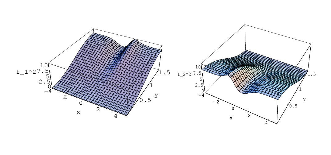
Refer to caption
Figure 2: Three-dimensional plot of the metric factor f12f_{1}^{2} and f22f_{2}^{2} for the supersymmetric Janus solution as function of xx and yy, for r=4r=4.
Refer to caption
Figure 3: Plot of the dilaton e4​ϕe^{4\phi} at y=0y=0 as a function of xx, for r=1.5r=1.5 (blue), r=2r=2 (red), r=3r=3 (magenta) and r=4r=4 (green).

The A​d​S4AdS_{4} metric factor is given by

ρ2​f42\displaystyle\rho^{2}f_{4}^{2} =\displaystyle= 4​N⁡(x,y)​D​(x,y)(ex+r​e−x)​(ex+e−x)\displaystyle 4\sqrt{{N(x,y)D(x,y)\over(e^{x}+re^{-x})(e^{x}+e^{-x})}} (10.23)

which is non-singular and nowhere vanishing. Taking the limit r→1r\rightarrow 1, we recover the A​d​S5×S5AdS_{5}\times S^{5} metric factors of (10.1).

10.4 The Half-BPS Janus holographic dual interface theory

The holographic interpretation of the original Janus solution is given by an interface conformal field theory. The dual four-dimensional field theory lives on two four-dimensional half spaces glued together at a three-dimensional interface. Although the Janus solution (10.14) is more complicated than the original [15] and the 𝒩=1{\cal N}=1 supersymmetric Janus solution [25], it shares many features with these solutions, as we shall show next. The asymptotic behavior of the metric functions can easily be obtained using the parametrization of the strip (10.13). In the limit x→±∞x\to\pm\infty one gets

ρ2\displaystyle\rho^{2} =\displaystyle= 2​(1+r)12+o⁡(e−2​|x|)\displaystyle\sqrt{2}(1+r)^{1\over 2}+o(e^{-2|x|})
f12\displaystyle f_{1}^{2} =\displaystyle= 4​2​(1+r)12​sin2⁡y+o⁡(e−2​|x|)\displaystyle 4\sqrt{2}(1+r)^{1\over 2}\sin^{2}y+o(e^{-2|x|})
f22\displaystyle f_{2}^{2} =\displaystyle= 4​2​(1+r)12​cos2⁡y+o⁡(e−2​|x|)\displaystyle 4\sqrt{2}(1+r)^{1\over 2}\cos^{2}y+o(e^{-2|x|})
f42\displaystyle f_{4}^{2} =\displaystyle= 2​2(1+r)12​e2​|x|+o⁡(1)\displaystyle{2\sqrt{2}\over(1+r)^{1\over 2}}e^{2|x|}+o(1) (10.24)

The boundary of the bulk geometry can be obtained by extracting the part of the space where the metric becomes infinite. It follows from (10.24) that the metric for A​d​S4AdS_{4} blows up when x→±∞x\to\pm\infty. There is however an additional component to the boundary. Employing the Poincaré patch metric for A​d​S4AdS_{4}.

d​sA​d​S42=1z2​(−d​t2+d​x12+d​x22+d​z2)ds_{AdS_{4}}^{2}={1\over z^{2}}\Big(-dt^{2}+dx_{1}^{2}+dx_{2}^{2}+dz^{2}\Big) (10.25)

it is obvious that there is another boundary component at z→0z\to 0. The ten-dimensional asymptotic metric, in the limit x→±∞,z→0x\to\pm\infty,z\to 0, is given by1212 12 Note that the metric on the strip is given by d​sΣ2=4​ρ2​(d​x2+d​y2)ds^{2}_{\Sigma}=4\rho^{2}(dx^{2}+dy^{2}) due to our slightly unconventional normalization of the two-dimensional frames ez,ez¯e^{z},e^{\bar{z}}.

d​s2\displaystyle ds^{2} ∼\displaystyle\sim 1z2​μ2​(z2​d​μ2+d​x12+d​x22−d​t2+d​z22​(1+r)CLOSE\displaystyle{1\over z^{2}\mu^{2}}\bigg(z^{2}d\mu^{2}+{dx_{1}^{2}+dx_{2}^{2}-dt^{2}+dz^{2}\over 2(1+r)} (10.26)
OPEN+z2​μ2​(d​y2+sin2⁡y​d​sS122+cos2⁡y​d​sS222))+o⁡(μ2)\displaystyle\qquad+z^{2}\mu^{2}(dy^{2}+\sin^{2}yds^{2}_{S_{1}^{2}}+\cos^{2}yds^{2}_{S_{2}^{2}})\bigg)+o(\mu^{2})

where a new local coordinate μ=e∓x\mu=e^{\mp x} was introduced. The limit x→±∞x\to\pm\infty corresponds to μ→0\mu\to 0. It follows from (10.26) that the boundary of the bulk geometry has three components: x→±∞x\to\pm\infty corresponds to two four-dimensional half spaces, which are glued together at a three-dimensional interface at z→0z\to 0. The structure of the boundary is therefore the same as in the original Janus solution and defines an interface field theory. The asymptotic behavior of the dilaton is

e2​ϕ\displaystyle e^{2\phi} =\displaystyle= e2​ϕ++o⁡(e−2​x),as​x→+∞\displaystyle e^{2\phi_{+}}+o(e^{-2x}),\;{\rm as}\;x\to+\infty
e2​ϕ\displaystyle e^{2\phi} =\displaystyle= e2​ϕ−+o⁡(e−2​x),as​x→−∞,\displaystyle e^{2\phi_{-}}+o(e^{-2x}),\;{\rm as}\;x\to-\infty, (10.27)

Hence the super Yang-Mills theory in the two half spaces has two different values of the coupling constant gY​Mg_{YM}, as in the original Janus solution. The NSNS and RR 2-form gauge potentials behave as follows near the boundary,

Re⁡(B(2))\displaystyle{\rm Re}(B_{(2)}) ∼\displaystyle\sim e−3​|x|​sin⁡y​e^45\displaystyle e^{-3|x|}\sin y\;\hat{e}^{45}
Im⁡(B(2))\displaystyle{\rm Im}(B_{(2)}) ∼\displaystyle\sim e−3​|x|​cos⁡y​e^67\displaystyle e^{-3|x|}\cos y\;\hat{e}^{67} (10.28)

Their dependence on the S5S^{5} corresponds to lowest Kaluza-Klein modes on the S5S^{5} of the anti-symmetric rank 2 tensor field and is associated with a scalar field of dimension Δ=3\Delta=3 [43, 44] in 𝒩=4{\cal N}=4 super-Yang-Mills.

The behavior (10.28) leads to a insertion of the dual operator which is localized at the interface. This agrees with the interpretation of the solution as a Janus interface CFT with an interface term given by (2.2). The detailed analysis is the same as the one given in [25] and will be repeated in the following for completeness.

In the following we will focus on one of the four-dimensional half spaces and use the local coordinate μ=e±x\mu=e^{\pm x} defined above (not to be confused with the harmonic function μ\mu introduced and used in subsection 9.1). The boundary is reached when μ​z→0\mu z\to 0. The complete boundary corresponds to two 4-dimensional half spaces joined by a 𝐑3{\bf R}^{3} interface located at z=0z=0.

The AdS/CFT correspondence relates 10-dimensional Type IIB supergravity fields to gauge invariant operators on the 𝒩=4{\cal N}=4 super Yang-Mills side. In the following we briefly review some aspects of this map. The Poincaré metric of Euclidean A​d​S5AdS_{5} is given by

d​s2=1z2​(d​z2+∑id​xi2)ds^{2}={1\over z^{2}}\left(dz^{2}+\sum_{i}dx_{i}^{2}\right) (10.29)

Near the boundary of A​d​S5AdS_{5}, where z→0z\to 0, a scalar field Φm\Phi_{m} of mass mm behaves as,

Φm​(z,x)∼ϕn​o​n−n​o​r​m​(x)​z4−Δ+ϕn​o​r​m​(x)​zΔ\Phi_{m}(z,x)\,\sim\,\phi_{non-norm}(x)z^{4-\Delta}+\phi_{norm}(x)z^{\Delta} (10.30)

where m2=Δ⁡(Δ−4)m^{2}=\Delta(\Delta-4). The non-normalizable mode corresponds to insertion in the Lagrangian of an operator 𝒪Δ{\cal O}_{\Delta} with scaling dimension Δ\Delta. The boundary source can be determined from (10.30) by

ϕn​o​n−n​o​r​m​(x)=limz→0zΔ−4​Φ​(z,x)\phi_{non-norm}(x)=\lim_{z\to 0}z^{\Delta-4}\Phi(z,x) (10.31)

If ϕn​o​n−n​o​r​m\phi_{non-norm} vanishes, a non-zero ϕn​o​r​m\phi_{norm} corresponds to a non-vanishing expectation value

⟨𝒪Δ⟩=ϕn​o​r​m\displaystyle\langle{\cal O}_{\Delta}\rangle=\phi_{norm} (10.32)

of the operators 𝒪Δ{\cal O}_{\Delta} on the Yang-Mills side. The asymptotic behavior near the boundary of the 2-form fields as μ→0\mu\to 0 is given by

b1​(μ)\displaystyle b_{1}(\mu) =\displaystyle= const​μ3+o⁡(μ5)\displaystyle{\rm const}\;\mu^{3}+o(\mu^{5})
b2​(μ)\displaystyle b_{2}(\mu) =\displaystyle= const​μ3+o⁡(μ5)\displaystyle{\rm const}\;\mu^{3}+o(\mu^{5}) (10.33)

The state operator correspondence (10.30) seems to suggest that there is no source for the Δ=3\Delta=3 operator dual to the 3-form fields, since the non-normalizable mode is not turned on. However, this conclusion is premature. For the Janus metric the appropriate rescaling of the field needed to extract the non-normalizable mode is given by

cn​o​n−n​o​r​m\displaystyle c_{non-norm} =\displaystyle= limϵ→0ϵΔ−4​c​(μ)\displaystyle\lim_{\epsilon\to 0}\epsilon^{\Delta-4}c(\mu) (10.34)
=\displaystyle= limϵ→01ϵ​μ3​const\displaystyle\lim_{\epsilon\to 0}{1\over\epsilon}\mu^{3}\;{\rm const}
=\displaystyle= limμ​z→0μ2z​const\displaystyle\lim_{\mu z\to 0}{\ \mu^{2}\over z}\;{\rm const}

where ϵ=μ​z\epsilon=\mu z was used. For a point on the boundary which is away from the three-dimensional interface one has z≠0z\neq 0 and it follows from (10.34) that the source for the dual operator vanishes away from the interface. However for the interface one has z=0z=0 and cn​o​n−n​o​r​mc_{non-norm} in (10.34) diverges. This behavior indicates the presence of a delta function source for the dual Δ=3\Delta=3 operator on the interface, since the integral over a small disk around the interface ∫d​μ​𝑑z​z​cn​o​n−n​o​r​m\int d\mu\;dzz\;c_{non-norm} is finite. The localized operator on the interface is the interface counterterm discussed in section 2, which is necessary to restore 𝒩=4{\cal N}=4 interface supersymmetry.

Acknowledgment

This work was supported in part by National Science Foundation (NSF) grant PHY-04-56200.

Appendix A Clifford algebra basis adapted to the Ansatz

We choose a basis for the Clifford algebra which is well-adapted to the A​d​S4×S12×S22×ΣAdS_{4}\times S_{1}^{2}\times S_{2}^{2}\times\Sigma Ansatz, with the frame labeled as in (4.1),

Γm\displaystyle\Gamma^{m} =\displaystyle= γm⊗I2⊗I2⊗I2m=0,1,2,3\displaystyle\gamma^{m}\otimes I_{2}\otimes I_{2}\otimes I_{2}\hskip 79.49744ptm=0,1,2,3
Γi1\displaystyle\Gamma^{i_{1}} =\displaystyle= γ(1)⊗γi1⊗I2⊗I2i1=4,5\displaystyle\gamma_{(1)}\otimes\gamma^{i_{1}}\otimes I_{2}\otimes I_{2}\hskip 72.26999pti_{1}=4,5
Γi2\displaystyle\Gamma^{i_{2}} =\displaystyle= γ(1)⊗σ3⊗γi2⊗I2i2=6,7\displaystyle\gamma_{(1)}\otimes\sigma^{3}\otimes\gamma^{i_{2}}\otimes I_{2}\hskip 72.26999pti_{2}=6,7
Γa\displaystyle\Gamma^{a}\, =\displaystyle= γ(1)⊗σ3⊗σ3⊗γaa=8,9\displaystyle\gamma_{(1)}\otimes\sigma^{3}\otimes\sigma^{3}\otimes\gamma^{a}\hskip 72.26999pta=8,9 (A.1)

where a convenient basis for the lower dimensional Clifford algebras is as follows,

i​γ0=σ2⊗I2\displaystyle i\gamma^{0}=\sigma^{2}\otimes I_{2} γ4=γ6=γ8=σ1\displaystyle\gamma^{4}=\gamma^{6}=\gamma^{8}=\sigma^{1}
γ1=σ1⊗I2\displaystyle\gamma^{1}=\sigma^{1}\otimes I_{2} γ5=γ7=γ9=σ2\displaystyle\gamma^{5}=\gamma^{7}=\gamma^{9}=\sigma^{2}
γ2=σ3⊗σ2\displaystyle\gamma^{2}=\sigma^{3}\otimes\sigma^{2}
γ3=σ3⊗σ1\displaystyle\gamma^{3}=\sigma^{3}\otimes\sigma^{1} (A.2)

We shall also need the chirality matrices on the various components of A​d​S4×S12×S22×ΣAdS_{4}\times S_{1}^{2}\times S_{2}^{2}\times\Sigma, and they are chosen as follows,

γ(1)\displaystyle\gamma_{(1)} =\displaystyle= −i​Γ0123=σ3⊗σ3⊗I2⊗I2⊗I2\displaystyle-i\Gamma^{0123}=\sigma^{3}\otimes\sigma^{3}\otimes I_{2}\otimes I_{2}\otimes I_{2}
γ(2)\displaystyle\gamma_{(2)} =\displaystyle= −i​Γ45=I2⊗I2⊗σ3⊗I2⊗I2\displaystyle-i\Gamma^{45}~~=I_{2}\otimes I_{2}\otimes\sigma^{3}\otimes I_{2}\otimes I_{2}
γ(3)\displaystyle\gamma_{(3)} =\displaystyle= −i​Γ67=I2⊗I2⊗I2⊗σ3⊗I2\displaystyle-i\Gamma^{67}~~=I_{2}\otimes I_{2}\otimes I_{2}\otimes\sigma^{3}\otimes I_{2}
γ(4)\displaystyle\gamma_{(4)} =\displaystyle= −i​Γ89=I2⊗I2⊗I2⊗I2⊗σ3\displaystyle-i\Gamma^{89}~~=I_{2}\otimes I_{2}\otimes I_{2}\otimes I_{2}\otimes\sigma^{3} (A.3)

The 10-dimensional chirality matrix in this basis is given by

Γ11=Γ0123456789=γ(1)​γ(2)​γ(3)​γ(4)\displaystyle\Gamma^{11}=\Gamma^{0123456789}=\gamma_{(1)}\gamma_{(2)}\gamma_{(3)}\gamma_{(4)} (A.4)

The complex conjugation matrices in each component are defined by

(γm)∗=+B(1)​γm​B(1)−1\displaystyle\left(\gamma^{m}\right)^{*}=+B_{(1)}\gamma^{m}B_{(1)}^{-1} (B(1))∗​B(1)=+I2B(1)=i​γ(1)​γ2\displaystyle(B_{(1)})^{*}B_{(1)}=+I_{2}\hskip 43.36243ptB_{(1)}=i\gamma_{(1)}\gamma^{2}
(γi1)∗=−B(2)​γi1​B(2)−1\displaystyle\left(\gamma^{i_{1}}\right)^{*}=-B_{(2)}\gamma^{i_{1}}B_{(2)}^{-1} (B(2))∗​B(2)=−I2B(2)=γ5\displaystyle(B_{(2)})^{*}B_{(2)}=-I_{2}\hskip 43.36243ptB_{(2)}=\gamma^{5}
(γi2)∗=−B(3)​γi2​B(3)−1\displaystyle\left(\gamma^{i_{2}}\right)^{*}=-B_{(3)}\gamma^{i_{2}}B_{(3)}^{-1} (B(3))∗​B(3)=−I2B(3)=γ7\displaystyle(B_{(3)})^{*}B_{(3)}=-I_{2}\hskip 43.36243ptB_{(3)}=\gamma^{7}
(γa)∗=−B(4)​γa​B(4)−1\displaystyle\left(\gamma^{a}\right)^{*}=-B_{(4)}\gamma^{a}B_{(4)}^{-1} (B(4))∗​B(4)=−I2B(4)=γ9\displaystyle(B_{(4)})^{*}B_{(4)}=-I_{2}\hskip 43.36243ptB_{(4)}=\gamma^{9} (A.5)

where in the last column we have also listed the form of these matrices in our particular basis. The 10-dimensional complex conjugation matrix ℬ{\cal B} is defined by (ΓM)∗=ℬ​ΓM​ℬ−1(\Gamma^{M})^{*}={\cal B}\Gamma^{M}{\cal B}^{-1} and ℬℬ∗=I{\cal B}{\cal B}^{*}=I, and in this basis is given by

ℬ=−Γ2579=i​γ(1)​γ2⊗γ5⊗γ6⊗γ9=i​B(1)⊗B(2)⊗(γ(3)​B(3))⊗B(4)\displaystyle{\cal B}=-\Gamma^{2579}=i\gamma_{(1)}\gamma^{2}\otimes\gamma^{5}\otimes\gamma^{6}\otimes\gamma^{9}=iB_{(1)}\otimes B_{(2)}\otimes\left(\gamma_{(3)}B_{(3)}\right)\otimes B_{(4)} (A.6)

Appendix B The geometry of Killing spinors

In this Appendix, we review the relation between the Killing spinor equation and the parallel transport equation in the presence of a flat connection with torsion on S2S^{2} and A​d​S4AdS_{4}.

B.1 The sphere S2S^{2}

On S2S^{2}, the Killing spinor equation is given by,

(∇i+η​12​σi​σ3)​ε\displaystyle\left(\nabla_{i}+\eta{1\over 2}\sigma_{i}\sigma_{3}\right)\varepsilon =\displaystyle= 0i=1,2\displaystyle 0\hskip 72.26999pti=1,2 (B.1)

where σ1,σ2,σ3\sigma^{1},\sigma^{2},\sigma^{3} are the standard Pauli matrices, and ∇i\nabla_{i} is the spin connection on S2S^{2}. (An equivalent equation is obtained by letting σi​σ3→i​σi\sigma_{i}\sigma_{3}\to i\sigma_{i} and ε′=e−iπσ3/4ε\varepsilon^{\prime}=e^{-i\pi\sigma_{3}/4}\varepsilon.) Integrability of this system of equations on the round sphere requires η=±1\eta=\pm 1.

The relevant flat connection with torsion is given by the Maurer-Cartan forms ω(t)\omega^{(t)} on S​O​(3)SO(3), in the spinor representation of S​O​(3)SO(3),

ω(t)=U†dU=14ωI​J(t)σ[IσJ]U∈SU(2)\displaystyle\omega^{(t)}=U^{\dagger}dU={1\over 4}\omega^{(t)}_{IJ}\,\sigma^{[I}\sigma^{J]}\hskip 72.26999ptU\in SU(2) (B.2)
d​ω(t)+ω(t)∧ω(t)=0\displaystyle d\omega^{(t)}+\omega^{(t)}\wedge\omega^{(t)}=0 (B.3)

where {σI,σJ}=2​δI​J\{\sigma_{I},\sigma_{J}\}=2\delta_{IJ}, with I,J=1,2,3I,J=1,2,3. The Maurer-Cartan equation (B.3) expresses the flatness of the connection ω(t)\omega^{(t)}, which in turn reflects the fact that S​O​(3)SO(3), like any Lie group, is paralellizable. Next, we view S2S^{2} as the coset space S2=S​O​(3)/S​O​(2)S^{2}=SO(3)/SO(2), and decompose the directions of the cotangent space of S​O​(3)SO(3) accordingly,

ω(t)=i2ωσ3+12eiσiσ3{ω≡ω12(t)ei≡ωi​3(t)i=1,2\displaystyle\omega^{(t)}={i\over 2}\omega\sigma_{3}+{1\over 2}e_{i}\sigma_{i}\sigma_{3}\hskip 72.26999pt\left\{\matrix{\omega\equiv\omega^{(t)}_{12}&\cr e_{i}\equiv\omega^{(t)}_{i3}&\quad i=1,2\cr}\right. (B.4)

where eie_{i} is the canonical frame, and ω\omega the canonical S​O​(2)SO(2) connection on S2S^{2}. The Maurer-Cartan equations imply the absence of torsion, and the constancy of curvature. The parallel transport equation for a 2-component spinor ε+\varepsilon_{+} is simply

(d+ω(t))​ε+=0\displaystyle\left(d+\omega^{(t)}\right)\varepsilon_{+}=0 (B.5)

On the one hand, using the identification ω(t)=U†​d​U\omega^{(t)}=U^{\dagger}dU, it may be solved trivially by

ε+=U†​ε0\displaystyle\varepsilon_{+}=U^{\dagger}\varepsilon_{0} (B.6)

where ε0\varepsilon_{0} is a constant spinor. On the other hand, using the canonical decomposition (B.4), and the expression for the covariant derivative in terms of forms, ei​∇i=d+i​ω​σ3/2e_{i}\nabla_{i}=d+i\omega\,\sigma_{3}/2, it is clear that the equation coincides with the Killing spinor equation with η=+1\eta=+1. The solution ε−\varepsilon_{-} to the Killing equation for η=−1\eta=-1 may be obtained from the solution ε+\varepsilon_{+}, by ε−=σ3​ε+\varepsilon_{-}=\sigma_{3}\,\varepsilon_{+}.

B.2 Minkowski A​d​S4AdS_{4}

The above construction may be generalized to all spheres and their hyperbolic counterparts. Here, we present the case of Minkowski signature A​d​S4=S​O​(2,3)/S​O​(1,3)AdS_{4}=SO(2,3)/SO(1,3). The Clifford algebra of S​O​(2,3)SO(2,3) is built from the Clifford generators γμ\gamma^{\mu}, of the Lorentz group S​O​(1,3)SO(1,3),

{γμ,γν}=2ημ​νη=diag[−+++]\displaystyle\{\gamma^{\mu},\gamma^{\nu}\}=2\eta^{\mu\nu}\hskip 72.26999pt\eta={\rm diag}[-+++] (B.7)

for μ,ν=0,1,2,3\mu,\nu=0,1,2,3, supplemented with the chirality matrix, γ♯≡γ0123\gamma^{\sharp}\equiv\gamma^{0123},

{γμ¯,γν¯}=2η¯μ¯​ν¯η¯=diag[−−+++]\displaystyle\{\gamma^{\bar{\mu}},\gamma^{\bar{\nu}}\}=2\bar{\eta}^{\bar{\mu}\bar{\nu}}\hskip 72.26999pt\bar{\eta}={\rm diag}[--+++] (B.8)

for μ¯,ν¯=♯,0,1,2,3\bar{\mu},\bar{\nu}=\sharp,0,1,2,3. The corresponding Maurer-Cartan form on S​O​(2,3)SO(2,3) is given by

ω(t)=V−1​d​V=14​ωμ¯​ν¯(t)​γμ¯​ν¯V∈S​p​(2,2)∼S​O​(2,3)\displaystyle\omega^{(t)}=V^{-1}dV={1\over 4}\omega^{(t)}_{\bar{\mu}\bar{\nu}}\gamma^{\bar{\mu}\bar{\nu}}\hskip 72.26999ptV\in Sp(2,2)\sim SO(2,3) (B.9)

It obviously satisfies the Maurer-Cartan equations, d​ω(t)+ω(t)∧ω(t)=0d\omega^{(t)}+\omega^{(t)}\wedge\omega^{(t)}=0. We decompose ω(t)\omega^{(t)} onto the S​O​(1,3)SO(1,3) and A​d​S4AdS_{4} directions of cotangent space,

ω(t)=14ωμ​νγμ​ν+i2eμγμγ(4){ωμ​ν≡ωμ​ν(t)μ,ν=0,1,2,3eμ≡ωμ​♯(t)μ=0,1,2,3\displaystyle\omega^{(t)}={1\over 4}\omega_{\mu\nu}\gamma^{\mu\nu}+{i\over 2}e_{\mu}\gamma^{\mu}\gamma_{(4)}\hskip 72.26999pt\left\{\matrix{\omega_{\mu\nu}\equiv\omega^{(t)}_{\mu\nu}&\mu,\nu=0,1,2,3\cr e_{\mu}\equiv\omega^{(t)}_{\mu\sharp}&\mu=0,1,2,3\cr}\right. (B.10)

The Maurer-Cartan equations d​ω(t)+ω(t)∧ω(t)=0d\omega^{(t)}+\omega^{(t)}\wedge\omega^{(t)}=0 for ω(t)\omega^{(t)} imply that the absence of torsion and that the constancy of curvature. The Killing spinor equation coincides with the equation for parallel transport,

(d+V−1​d​V)​ε=(d+14​ωμ​ν​γμ​ν+i2​η​eμ​γμ​γ(4))​ε=0\displaystyle\left(d+V^{-1}dV\right)\varepsilon=\left(d+{1\over 4}\omega_{\mu\nu}\gamma^{\mu\nu}+{i\over 2}\eta e_{\mu}\gamma^{\mu}\gamma_{(4)}\right)\varepsilon=0 (B.11)

For η=+1\eta=+1, the general solution is given by ε+=V−1​ε0\varepsilon_{+}=V^{-1}\varepsilon_{0} and ε0\varepsilon_{0} is constant, while for η=−1\eta=-1, the solution is ε−=γ♯​ε+\varepsilon_{-}=\gamma^{\sharp}\varepsilon_{+}. Note that VV is a symplectic matrix, so that Vt​J​V=JV^{t}JV=J, and this allows us to define an invariant inner product on the spinors.

Appendix C The derivation of the BPS equations

We begin by collecting some identities that will be useful during the reduction of the BPS equations over the Ansatz of subsection 4.1. The Clifford algebra matrices needed are,

Γa\displaystyle\Gamma^{a} =\displaystyle= γ(1)​γ(2)​γ(3)​γa\displaystyle\gamma_{(1)}\gamma_{(2)}\gamma_{(3)}\gamma^{a}
Γ45​a\displaystyle\Gamma^{45a} =\displaystyle= i​γ(1)​γ(3)​γa\displaystyle i\gamma_{(1)}\gamma_{(3)}\gamma^{a}
Γ67​a\displaystyle\Gamma^{67a} =\displaystyle= i​γ(1)​γ(2)​γa\displaystyle i\gamma_{(1)}\gamma_{(2)}\gamma^{a}
Γ0123​a\displaystyle\Gamma^{0123a} =\displaystyle= i​γ(2)​γ(3)​γa\displaystyle i\gamma_{(2)}\gamma_{(3)}\gamma^{a}
εa​b​Γ4567​b\displaystyle\varepsilon^{ab}\Gamma^{4567b} =\displaystyle= −γ(1)​εa​b​γb\displaystyle-\gamma_{(1)}\varepsilon^{ab}\gamma^{b} (C.1)

We shall also need the following decompositions of ε\varepsilon and ℬ−1​ε∗{\cal B}^{-1}\varepsilon^{*},

ε\displaystyle\varepsilon =\displaystyle= ∑η1,η2,η3χη1,η2,η3⊗ζη1,η2,η3\displaystyle\sum_{\eta_{1},\eta_{2},\eta_{3}}\chi^{\eta_{1},\eta_{2},\eta_{3}}\otimes\zeta_{\eta_{1},\eta_{2},\eta_{3}}
ℬ−1​ε∗\displaystyle{\cal B}^{-1}\varepsilon^{*} =\displaystyle= ∑η1,η2,η3χη1,η2,η3⊗∗ζη1,η2,η3\displaystyle\sum_{\eta_{1},\eta_{2},\eta_{3}}\chi^{\eta_{1},\eta_{2},\eta_{3}}\otimes*\zeta_{\eta_{1},\eta_{2},\eta_{3}} (C.2)

where we use the abbreviation,

∗ζη1,η2,η3\displaystyle*\zeta_{\eta_{1},\eta_{2},\eta_{3}} =\displaystyle= −i​σ2​η1​η2​η3​ζη1,η2,−η3∗\displaystyle-i\sigma^{2}\eta_{1}\eta_{2}\eta_{3}\zeta_{\eta_{1},\eta_{2},-\eta_{3}}^{*}
∗ζ\displaystyle{}*\zeta =\displaystyle= τ332⊗σ2​ζ∗\displaystyle\tau^{332}\otimes\sigma^{2}\zeta^{*} (C.3)

in τ\tau-matrix notation.

C.1 The dilatino equation

The dilatino equation is,

0=i​PA​ΓA​ℬ−1​ε∗−i24​Γ⋅G​ε\displaystyle 0=iP_{A}\Gamma^{A}{\cal B}^{-1}\varepsilon^{*}-{i\over 24}\Gamma\cdot G\varepsilon (C.4)

Reduced to the Ansatz of subsection 4.1, we have the following simplifications,

PA​ΓA\displaystyle P_{A}\Gamma^{A} =\displaystyle= pa​Γa\displaystyle p_{a}\Gamma^{a}
Γ⋅G\displaystyle\Gamma\cdot G =\displaystyle= 3!​(ga​Γ45​a+i​ha​Γ67​a)\displaystyle 3!(g_{a}\Gamma^{45a}+i\,h_{a}\Gamma^{67a}) (C.5)

The dilatino equation now becomes,

0\displaystyle 0 =\displaystyle= i​pa​Γa​∑η1,η2,η3χη1,η2,η3​(−i​σ2)​η1​η2​η3​ζη1,η2,−η3∗\displaystyle ip_{a}\Gamma^{a}\sum_{\eta_{1},\eta_{2},\eta_{3}}\chi^{\eta_{1},\eta_{2},\eta_{3}}(-i\sigma^{2})\eta_{1}\eta_{2}\eta_{3}\zeta_{\eta_{1},\eta_{2},-\eta_{3}}^{*} (C.6)
−i4(gaΓ45​a+ihaΓ67​a)∑η1,η2,η3χη1,η2,η3⊗ζη1,η2,η3\displaystyle-{i\over 4}(g_{a}\Gamma^{45a}+i\,h_{a}\Gamma^{67a})\sum_{\eta_{1},\eta_{2},\eta_{3}}\chi^{\eta_{1},\eta_{2},\eta_{3}}\otimes\zeta_{\eta_{1},\eta_{2},\eta_{3}}

Using the above form of the Γ\Gamma-matrices, the action of the chirality matrices on χ\chi, and flipping the signs in the summation over η\eta so as to have a common factor of χ\chi, we obtain,

0=∑η1,η2,η3χη1,η2,η3⊗(−pa​σa​σ2​η1​η2​η3​ζ−η1,−η2,η3∗+14​ga​σa​ζ−η1,η2,−η3+i4​ha​σa​ζ−η1,−η2,η3)\displaystyle 0=\sum_{\eta_{1},\eta_{2},\eta_{3}}\chi^{\eta_{1},\eta_{2},\eta_{3}}\otimes\bigg(-p_{a}\sigma^{a}\sigma^{2}\eta_{1}\eta_{2}\eta_{3}\zeta_{-\eta_{1},-\eta_{2},\eta_{3}}^{*}+{1\over 4}g_{a}\sigma^{a}\zeta_{-\eta_{1},\eta_{2},-\eta_{3}}+{i\over 4}h_{a}\sigma^{a}\zeta_{-\eta_{1},-\eta_{2},\eta_{3}}\bigg) (C.7)

Since the χη1,η2,η3\chi^{\eta_{1},\eta_{2},\eta_{3}} are linearly independent we require the vanishing of

0=−pa​σa​σ2​η1​η2​η3​ζ−η1,−η2,η3∗+14​ga​σa​ζ−η1,η2,−η3+i4​ha​σa​ζ−η1,−η2,η3\displaystyle 0=-p_{a}\sigma^{a}\sigma^{2}\eta_{1}\eta_{2}\eta_{3}\zeta_{-\eta_{1},-\eta_{2},\eta_{3}}^{*}+{1\over 4}g_{a}\sigma^{a}\zeta_{-\eta_{1},\eta_{2},-\eta_{3}}+{i\over 4}h_{a}\sigma^{a}\zeta_{-\eta_{1},-\eta_{2},\eta_{3}} (C.8)

This can be recast economically using the τ\tau-matrix notation,

0=pa​τ(223)​σa​σ2​ζ∗+14​ga​τ(101)​σa​ζ+i4​ha​τ(110)​σa​ζ\displaystyle 0=p_{a}\tau^{(223)}\sigma^{a}\sigma^{2}\zeta^{*}+{1\over 4}g_{a}\tau^{(101)}\sigma^{a}\zeta+{i\over 4}h_{a}\tau^{(110)}\sigma^{a}\zeta (C.9)

Upon multiplication on the left by τ(223)\tau^{(223)}, we recover (5.9).

C.2 The gravitino equation

The gravitino equation is

0\displaystyle 0 =\displaystyle= d​ε+ω​ε+ϕ​ε+g​ℬ−1​ε∗\displaystyle d\varepsilon+\omega\varepsilon+\phi\varepsilon+g{\cal B}^{-1}\varepsilon^{*}
ω\displaystyle\omega =\displaystyle= 14​ωA​B​ΓA​B\displaystyle{1\over 4}\omega_{AB}\Gamma^{AB}
ϕ\displaystyle\phi =\displaystyle= −i2​Q+i480​(Γ⋅F(5))​eA​ΓA\displaystyle-{i\over 2}Q+{i\over 480}(\Gamma\cdot F_{(5)})e_{A}\Gamma^{A}
g\displaystyle g =\displaystyle= −196​eA​(ΓA​(Γ⋅G)+2​(Γ⋅G)​ΓA)\displaystyle-{1\over 96}e_{A}\bigg(\Gamma^{A}(\Gamma\cdot G)+2(\Gamma\cdot G)\Gamma^{A}\bigg) (C.10)

C.2.1 The calculation of ω\omega

The spin connection components are ωab\omega^{a}{}_{b}, whose explicit form we shall not need, and

ωmn=ω^mn\displaystyle\omega^{m}{}_{n}=\hat{\omega}^{m}{}_{n} ωma=em∂af4f4\displaystyle\omega^{m}{}_{a}=e^{m}{\partial_{a}f_{4}\over f_{4}}
ωi1i2=ω^i1i2\displaystyle\omega^{i_{1}}{}_{i_{2}}=\hat{\omega}^{i_{1}}{}_{i_{2}} ωi1a=ei1∂af1f1\displaystyle\omega^{i_{1}}{}_{a}=e^{i_{1}}{\partial_{a}f_{1}\over f_{1}}
ωi2j2=ω^i2j2\displaystyle\omega^{i_{2}}{}_{j_{2}}=\hat{\omega}^{i_{2}}{}_{j_{2}} ωi2a=ei2∂af2f2\displaystyle\omega^{i_{2}}{}_{a}=e^{i_{2}}{\partial_{a}f_{2}\over f_{2}} (C.11)

The hats refers to the canonical connections on A​d​S4AdS_{4}, S12S^{2}_{1}, S22S^{2}_{2} respectively. Projecting the spin-connection along the various directions we have

(m)\displaystyle(m) ∇m′ε+12​Da​f4f4​Γm​Γa​ε\displaystyle\nabla_{m}^{\prime}\varepsilon+{1\over 2}{D_{a}f_{4}\over f_{4}}\Gamma_{m}\Gamma^{a}\varepsilon
(i1)\displaystyle(i_{1}) ∇i1′ε+12​Da​f1f1​Γi1​Γa​ε\displaystyle\nabla_{i_{1}}^{\prime}\varepsilon+{1\over 2}{D_{a}f_{1}\over f_{1}}\Gamma_{i_{1}}\Gamma^{a}\varepsilon
(i2)\displaystyle(i_{2}) ∇i2′ε+12​Da​f2f2​Γi2​Γa​ε\displaystyle\nabla_{i_{2}}^{\prime}\varepsilon+{1\over 2}{D_{a}f_{2}\over f_{2}}\Gamma_{i_{2}}\Gamma^{a}\varepsilon
(a)\displaystyle(a) ∇aε\displaystyle\nabla_{a}\varepsilon (C.12)

where the prime on the covariant derivative indicates that only the connection along A​d​S4AdS_{4}, S12S^{2}_{1} or S22S^{2}_{2} respectively is included. Using the Killing spinor equations (5.1) we can eliminate the primed covariant derivatives, which yields

(m)\displaystyle(m) 12​f4​Γm​∑η1,η2,η3η1​χη1,η2,η3⊗ζη1,η2,η3+12​Da​f4f4​Γm​Γa​ε\displaystyle{1\over 2f_{4}}\Gamma_{m}\sum_{\eta_{1},\eta_{2},\eta_{3}}\eta_{1}\chi^{\eta_{1},\eta_{2},\eta_{3}}\otimes\zeta_{\eta_{1},\eta_{2},\eta_{3}}+{1\over 2}{D_{a}f_{4}\over f_{4}}\Gamma_{m}\Gamma^{a}\varepsilon
(i1)\displaystyle(i_{1}) i2​f1​Γi1​γ(1)​∑η1,η2,η3η2​χη1,η2,η3⊗ζη1,η2,η3+12​Da​f1f1​Γi1​Γa​ϵ\displaystyle{i\over 2f_{1}}\Gamma_{i_{1}}\gamma_{(1)}\sum_{\eta_{1},\eta_{2},\eta_{3}}\eta_{2}\chi^{\eta_{1},\eta_{2},\eta_{3}}\otimes\zeta_{\eta_{1},\eta_{2},\eta_{3}}+{1\over 2}{D_{a}f_{1}\over f_{1}}\Gamma_{i_{1}}\Gamma^{a}\epsilon
(i2)\displaystyle(i_{2}) i2​f2​Γi2​γ(1)​γ(2)​∑η1,η2,η3η3​χη1,η2,η3⊗ζη1,η2,η3+12​Da​f2f2​Γi2​Γa​ε\displaystyle{i\over 2f_{2}}\Gamma_{i_{2}}\gamma_{(1)}\gamma_{(2)}\sum_{\eta_{1},\eta_{2},\eta_{3}}\eta_{3}\chi^{\eta_{1},\eta_{2},\eta_{3}}\otimes\zeta_{\eta_{1},\eta_{2},\eta_{3}}+{1\over 2}{D_{a}f_{2}\over f_{2}}\Gamma_{i_{2}}\Gamma^{a}\varepsilon (C.13)

Using the equation Γa=γ(1)​γ(2)​γ(3)​σa\Gamma^{a}=\gamma_{(1)}\gamma_{(2)}\gamma_{(3)}\sigma^{a}, we have

(m)\displaystyle(m) Γm​∑η1,η2,η3χη1,η2,η3⊗(12​f4​η1​ζη1,η2,η3+12​Da​f4f4​σa​ζ−η1,−η2,−η3)\displaystyle\Gamma_{m}\sum_{\eta_{1},\eta_{2},\eta_{3}}\chi^{\eta_{1},\eta_{2},\eta_{3}}\otimes\bigg({1\over 2f_{4}}\eta_{1}\zeta_{\eta_{1},\eta_{2},\eta_{3}}+{1\over 2}{D_{a}f_{4}\over f_{4}}\sigma^{a}\zeta_{-\eta_{1},-\eta_{2},-\eta_{3}}\bigg)
(i1)\displaystyle(i_{1}) Γi1​∑η1,η2,η3χη1,η2,η3⊗(i2​f1​η2​ζ−η1,η2,η3+12​Da​f1f1​σa​ζ−η1,−η2,−η3)\displaystyle\Gamma_{i_{1}}\sum_{\eta_{1},\eta_{2},\eta_{3}}\chi^{\eta_{1},\eta_{2},\eta_{3}}\otimes\bigg({i\over 2f_{1}}\eta_{2}\zeta_{-\eta_{1},\eta_{2},\eta_{3}}+{1\over 2}{D_{a}f_{1}\over f_{1}}\sigma^{a}\zeta_{-\eta_{1},-\eta_{2},-\eta_{3}}\bigg)
(i2)\displaystyle(i_{2}) Γi2​∑η1,η2,η3χη1,η2,η3⊗(i2​f2​η3​ζ−η1,−η2,η3+12​Da​f2f2​σa​ζ−η1,−η2,−η3)\displaystyle\Gamma_{i_{2}}\sum_{\eta_{1},\eta_{2},\eta_{3}}\chi^{\eta_{1},\eta_{2},\eta_{3}}\otimes\bigg({i\over 2f_{2}}\eta_{3}\zeta_{-\eta_{1},-\eta_{2},\eta_{3}}+{1\over 2}{D_{a}f_{2}\over f_{2}}\sigma^{a}\zeta_{-\eta_{1},-\eta_{2},-\eta_{3}}\bigg) (C.14)

where we have pulled a factor of ΓM\Gamma_{M} out front. It will turn out that all terms in the gravitino equation contain ΓM​χη1,η2,η3\Gamma_{M}\chi^{\eta_{1},\eta_{2},\eta_{3}}, and we will require the coefficients to vanish independently, just as we did for the dilatino equation. The coefficient of ΓM​χη1,η2,η3\Gamma_{M}\chi^{\eta_{1},\eta_{2},\eta_{3}} can be expressed in the τ\tau-matrix notation as

(m)\displaystyle(m) 12​f4​τ(300)​ζ+12​Da​f4f4​τ(111)​σa​ζ\displaystyle{1\over 2f_{4}}\tau^{(300)}\zeta+{1\over 2}{D_{a}f_{4}\over f_{4}}\tau^{(111)}\sigma^{a}\zeta
(i1)\displaystyle(i_{1}) i2​f1​τ(130)​ζ+12​Da​f1f1​τ(111)​σa​ζ\displaystyle{i\over 2f_{1}}\tau^{(130)}\zeta+{1\over 2}{D_{a}f_{1}\over f_{1}}\tau^{(111)}\sigma^{a}\zeta
(i2)\displaystyle(i_{2}) i2​f2​τ(113)​ζ+12​Da​f2f2​τ(111)​σa​ζ\displaystyle{i\over 2f_{2}}\tau^{(113)}\zeta+{1\over 2}{D_{a}f_{2}\over f_{2}}\tau^{(111)}\sigma^{a}\zeta (C.15)

C.2.2 The calculation of ϕ\phi

The QQ part is trivial. The F(5)F_{(5)} part is

i480​(Γ⋅F(5))​ΓA​eA​ε=−i2​fa​Γ0123​a​ΓA​eA​ε\displaystyle{i\over 480}(\Gamma\cdot F_{(5)})\Gamma^{A}e_{A}\varepsilon=-{i\over 2}f_{a}\Gamma^{0123a}\Gamma^{A}e_{A}\varepsilon (C.16)

Projecting along the various directions, we have

(m)\displaystyle(m) Γm​∑η1,η2,η3χη1,η2,η3⊗12​fa​σa​ζη1,−η2,−η3\displaystyle\Gamma_{m}\sum_{\eta_{1},\eta_{2},\eta_{3}}\chi^{\eta_{1},\eta_{2},\eta_{3}}\otimes{1\over 2}f_{a}\sigma^{a}\zeta_{\eta_{1},-\eta_{2},-\eta_{3}}
(i1)\displaystyle(i_{1}) −Γi1∑η1,η2,η3χη1,η2,η3⊗12faσaζη1,−η2,−η3\displaystyle-\Gamma_{i_{1}}\sum_{\eta_{1},\eta_{2},\eta_{3}}\chi^{\eta_{1},\eta_{2},\eta_{3}}\otimes{1\over 2}f_{a}\sigma^{a}\zeta_{\eta_{1},-\eta_{2},-\eta_{3}}
(i2)\displaystyle(i_{2}) −Γi2∑η1,η2,η3χη1,η2,η3⊗12faσaζη1,−η2,−η3\displaystyle-\Gamma_{i_{2}}\sum_{\eta_{1},\eta_{2},\eta_{3}}\chi^{\eta_{1},\eta_{2},\eta_{3}}\otimes{1\over 2}f_{a}\sigma^{a}\zeta_{\eta_{1},-\eta_{2},-\eta_{3}}
(a)\displaystyle(a) ∑η1,η2,η3χη1,η2,η3⊗(−i​Q2​ζη1,η2,η3+12​fb​σb​σa​ζ−η1,η2,η3)\displaystyle\sum_{\eta_{1},\eta_{2},\eta_{3}}\chi^{\eta_{1},\eta_{2},\eta_{3}}\otimes\bigg(-{iQ\over 2}\zeta_{\eta_{1},\eta_{2},\eta_{3}}+{1\over 2}f_{b}\sigma^{b}\sigma_{a}\zeta_{-\eta_{1},\eta_{2},\eta_{3}}\bigg) (C.17)

Using the τ\tau-matrix notation, we can write the coefficient of ΓM​χη1,η2,η3\Gamma_{M}\chi^{\eta_{1},\eta_{2},\eta_{3}} in the form

(m)\displaystyle(m) 12​fa​τ(011)⊗σa​ζ\displaystyle{1\over 2}f_{a}\tau^{(011)}\otimes\sigma^{a}\zeta (C.18)
(i1)\displaystyle(i_{1}) −12faτ(011)⊗σaζ\displaystyle-{1\over 2}f_{a}\tau^{(011)}\otimes\sigma^{a}\zeta
(i2)\displaystyle(i_{2}) −12faτ(011)⊗σaζ\displaystyle-{1\over 2}f_{a}\tau^{(011)}\otimes\sigma^{a}\zeta
(a)\displaystyle(a) −i​qa2​ζ+12​fb​τ(100)⊗σb​σa​ζ\displaystyle-{iq_{a}\over 2}\zeta+{1\over 2}f_{b}\tau^{(100)}\otimes\sigma^{b}\sigma_{a}\zeta

where qaq_{a} is defined by Q=qa​eaQ=q_{a}e^{a}.

C.2.3 The calculation of gg

The relevant expression is as follows,

g​ℬ−1​ϵ∗=−3!96​eA​(ga​(ΓA​Γ45​a+2​Γ45​a​ΓA)+i​ha​(ΓA​Γ67​a+2​Γ67​a​ΓA))​ℬ−1​ϵ∗\displaystyle g{\cal B}^{-1}\epsilon^{*}=-{3!\over 96}e_{A}\bigg(g_{a}(\Gamma^{A}\Gamma^{45a}+2\Gamma^{45a}\Gamma^{A})+ih_{a}(\Gamma^{A}\Gamma^{67a}+2\Gamma^{67a}\Gamma^{A})\bigg){\cal B}^{-1}\epsilon^{*} (C.19)

A few useful equations are as follows,

Γa​Γ45​b+2​Γ45​b​Γa\displaystyle\Gamma^{a}\Gamma^{45b}+2\Gamma^{45b}\Gamma^{a} =\displaystyle= Γ45​(3​δa​b−Γa​b)=i​γ(2)​(3​δa​b−σa​b)\displaystyle\Gamma^{45}(3\delta^{ab}-\Gamma^{ab})=i\gamma_{(2)}(3\delta^{ab}-\sigma^{ab})
Γa​Γ67​b+2​Γ67​b​Γa\displaystyle\Gamma^{a}\Gamma^{67b}+2\Gamma^{67b}\Gamma^{a} =\displaystyle= Γ67​(3​δa​b−Γa​b)=i​γ(3)​(3​δa​b−σa​b)\displaystyle\Gamma^{67}(3\delta^{ab}-\Gamma^{ab})=i\gamma_{(3)}(3\delta^{ab}-\sigma^{ab}) (C.20)

Projecting along the various directions we obtain

(m)\displaystyle(m) −Γm∑η1,η2,η3χη1,η2,η3⊗116(−igaσa∗ζ−η1,η2,−η3+haσa∗ζ−η1,−η2,η3)\displaystyle-\Gamma_{m}\sum_{\eta_{1},\eta_{2},\eta_{3}}\chi^{\eta_{1},\eta_{2},\eta_{3}}\otimes{1\over 16}(-ig_{a}\sigma^{a}*\zeta_{-\eta_{1},\eta_{2},-\eta_{3}}+h_{a}\sigma^{a}*\zeta_{-\eta_{1},-\eta_{2},\eta_{3}}) (C.21)
(i1)\displaystyle(i_{1}) −Γi1∑η1,η2,η3χη1,η2,η3⊗116(3igaσa∗ζ−η1,η2,−η3+haσa∗ζ−η1,−η2,η3)\displaystyle-\Gamma_{i_{1}}\sum_{\eta_{1},\eta_{2},\eta_{3}}\chi^{\eta_{1},\eta_{2},\eta_{3}}\otimes{1\over 16}(3ig_{a}\sigma^{a}*\zeta_{-\eta_{1},\eta_{2},-\eta_{3}}+h_{a}\sigma^{a}*\zeta_{-\eta_{1},-\eta_{2},\eta_{3}})
(i2)\displaystyle(i_{2}) −Γi2∑η1,η2,η3χη1,η2,η3⊗116(−igaσa∗ζ−η1,η2,−η3−3haσa∗ζ−η1,−η2,η3)\displaystyle-\Gamma_{i_{2}}\sum_{\eta_{1},\eta_{2},\eta_{3}}\chi^{\eta_{1},\eta_{2},\eta_{3}}\otimes{1\over 16}(-ig_{a}\sigma^{a}*\zeta_{-\eta_{1},\eta_{2},-\eta_{3}}-3h_{a}\sigma^{a}*\zeta_{-\eta_{1},-\eta_{2},\eta_{3}})
(a)\displaystyle(a) −∑η1,η2,η3χη1,η2,η3⊗116(3iga∗ζη1,−η2,η3−igbσa​b∗ζη1,−η2,η3\displaystyle-\sum_{\eta_{1},\eta_{2},\eta_{3}}\chi^{\eta_{1},\eta_{2},\eta_{3}}\otimes{1\over 16}\bigg(3ig_{a}*\zeta_{\eta_{1},-\eta_{2},\eta_{3}}-ig_{b}\sigma^{ab}*\zeta_{\eta_{1},-\eta_{2},\eta_{3}}
−3ha∗ζη1,η2,−η3+haσa​b∗ζη1,η2,−η3)\displaystyle\hskip 108.405pt-3h_{a}*\zeta_{\eta_{1},\eta_{2},-\eta_{3}}+h_{a}\sigma^{ab}*\zeta_{\eta_{1},\eta_{2},-\eta_{3}}\bigg)

Using the τ\tau-matrix notation, we can write the coefficient of ΓM​χη1,η2,η3\Gamma_{M}\chi^{\eta_{1},\eta_{2},\eta_{3}} in the form

(m)\displaystyle(m) −116(−igaτ(101)σa∗ζ+haτ(110)σa∗ζ)\displaystyle-{1\over 16}(-ig_{a}\tau^{(101)}\sigma^{a}*\zeta+h_{a}\tau^{(110)}\sigma^{a}*\zeta) (C.22)
(i1)\displaystyle(i_{1}) −116​(3​i​ga​τ(101)​σa∗ζ+ha​τ(110)​σa∗ζ)\displaystyle-{1\over 16}(3ig_{a}\tau^{(101)}\sigma^{a}*\zeta+h_{a}\tau^{(110)}\sigma^{a}*\zeta)
(i2)\displaystyle(i_{2}) −116(−igaτ(101)σa∗ζ−3haτ(110)σa∗ζ)\displaystyle-{1\over 16}(-ig_{a}\tau^{(101)}\sigma^{a}*\zeta-3h_{a}\tau^{(110)}\sigma^{a}*\zeta)
(a)\displaystyle(a) −116​(3​i​ga​τ(010)∗ζ−i​gb​τ(010)​σa​b∗ζ−3​ha​τ(001)∗ζ+ha​τ(001)​σa​b∗ζ)\displaystyle-{1\over 16}\bigg(3ig_{a}\tau^{(010)}*\zeta-ig_{b}\tau^{(010)}\sigma^{ab}*\zeta-3h_{a}\tau^{(001)}*\zeta+h_{a}\tau^{(001)}\sigma^{ab}*\zeta\bigg)

C.2.4 Assembling the complete gravitino BPS equation

Now we combine the three equations (C.2.1)(\ref{redomega}), (C.18)(\ref{redphi}), and (C.22)(\ref{redg}) to obtain the reduced gravitino equations. We again argue that the ΓM​χη1​η2​η3\Gamma_{M}\chi^{\eta_{1}\eta_{2}\eta_{3}} are linearly independent which leads to the equations

(m)\displaystyle(m) 0=12​f4​τ(300)​ζ+12​Da​f4f4​τ(111)​σa​ζ+12​fa​τ(011)​σa​ζ\displaystyle 0={1\over 2f_{4}}\tau^{(300)}\zeta+{1\over 2}{D_{a}f_{4}\over f_{4}}\tau^{(111)}\sigma^{a}\zeta+{1\over 2}f_{a}\tau^{(011)}\sigma^{a}\zeta
+116igaτ(101)σa∗ζ−116haτ(110)σa∗ζ\displaystyle\hskip 28.90755pt+{1\over 16}ig_{a}\tau^{(101)}\sigma^{a}*\zeta-{1\over 16}h_{a}\tau^{(110)}\sigma^{a}*\zeta
(i1)\displaystyle(i_{1}) 0=i2​f1​τ(130)​ζ+12​Da​f1f1​τ(111)​σa​ζ−12​fa​τ(011)​σa​ζ\displaystyle 0={i\over 2f_{1}}\tau^{(130)}\zeta+{1\over 2}{D_{a}f_{1}\over f_{1}}\tau^{(111)}\sigma^{a}\zeta-{1\over 2}f_{a}\tau^{(011)}\sigma^{a}\zeta
−316igaτ(101)σa∗ζ−116haτ(110)σa∗ζ\displaystyle\hskip 28.90755pt-{3\over 16}ig_{a}\tau^{(101)}\sigma^{a}*\zeta-{1\over 16}h_{a}\tau^{(110)}\sigma^{a}*\zeta
(i2)\displaystyle(i_{2}) 0=i2​f2​τ(113)​ζ+12​Da​f2f2​τ(111)​σa​ζ−12​fa​τ(011)​σa​ζ\displaystyle 0={i\over 2f_{2}}\tau^{(113)}\zeta+{1\over 2}{D_{a}f_{2}\over f_{2}}\tau^{(111)}\sigma^{a}\zeta-{1\over 2}f_{a}\tau^{(011)}\sigma^{a}\zeta
+116igaτ(101)σa∗ζ+316haτ(110)σa∗ζ\displaystyle\hskip 28.90755pt+{1\over 16}ig_{a}\tau^{(101)}\sigma^{a}*\zeta+{3\over 16}h_{a}\tau^{(110)}\sigma^{a}*\zeta
(a)\displaystyle(a) 0=(Da+i2​ω^a​σ3)​ζ−i2​qa​ζ+12​fb​τ(100)​σb​σa​ζ\displaystyle 0=\bigg(D_{a}+{i\over 2}\hat{\omega}_{a}\sigma^{3}\bigg)\zeta-{i\over 2}q_{a}\zeta+{1\over 2}f_{b}\tau^{(100)}\sigma^{b}\sigma_{a}\zeta (C.23)
−316igaτ(010)∗ζ+116igbτ(010)σa​b∗ζ\displaystyle\hskip 28.90755pt-{3\over 16}ig_{a}\tau^{(010)}*\zeta+{1\over 16}ig_{b}\tau^{(010)}\sigma^{ab}*\zeta
+316haτ(001)∗ζ−116hbτ(001)σa​b∗ζ\displaystyle\hskip 28.90755pt+{3\over 16}h_{a}\tau^{(001)}*\zeta-{1\over 16}h_{b}\tau^{(001)}\sigma^{ab}*\zeta

where ω^a=(ω^89)a\hat{\omega}_{a}=(\hat{\omega}_{89})_{a} is the spin connection along Σ\Sigma. In the first three equations, we have dropped an overall factor of ΓM\Gamma_{M}. In the last equation, we have used the connection formula (C.2.1)(\ref{spincon}) for the covariant derivative and the fact Γ89=i​σ3\Gamma^{89}=i\,\sigma^{3}. Eliminating the star using the definition (C)(\ref{star}), ∗ζ=τ(332)⊗σ2​ζ∗*\zeta=\tau^{(332)}\otimes\sigma^{2}\zeta^{*}. The system of gravitino BPS equations is then

(m)\displaystyle(m) 0=12​f4​τ(300)​ζ+12​∂af4f4​τ(111)​σa​ζ+12​fa​τ(011)​σa​ζ\displaystyle 0={1\over 2f_{4}}\tau^{(300)}\zeta+{1\over 2}{\partial_{a}f_{4}\over f_{4}}\tau^{(111)}\sigma^{a}\zeta+{1\over 2}f_{a}\tau^{(011)}\sigma^{a}\zeta
+116​i​ga​τ(233)​σa​σ2​ζ∗+116​ha​τ(222)​σa​σ2​ζ∗\displaystyle\hskip 28.90755pt+{1\over 16}ig_{a}\tau^{(233)}\sigma^{a}\sigma^{2}\zeta^{*}+{1\over 16}h_{a}\tau^{(222)}\sigma^{a}\sigma^{2}\zeta^{*}
(i1)\displaystyle(i_{1}) 0=i2​f1​τ(130)​ζ+12​∂af1f1​τ(111)​σa​ζ−12​fa​τ(011)​σa​ζ\displaystyle 0={i\over 2f_{1}}\tau^{(130)}\zeta+{1\over 2}{\partial_{a}f_{1}\over f_{1}}\tau^{(111)}\sigma^{a}\zeta-{1\over 2}f_{a}\tau^{(011)}\sigma^{a}\zeta
−316​i​ga​τ(233)​σa​σ2​ζ∗+116​ha​τ(222)​σa​σ2​ζ∗\displaystyle\hskip 28.90755pt-{3\over 16}ig_{a}\tau^{(233)}\sigma^{a}\sigma^{2}\zeta^{*}+{1\over 16}h_{a}\tau^{(222)}\sigma^{a}\sigma^{2}\zeta^{*}
(i2)\displaystyle(i_{2}) 0=i2​f2​τ(113)​ζ+12​∂af2f2​τ(111)​σa​ζ−12​fa​τ(011)​σa​ζ\displaystyle 0={i\over 2f_{2}}\tau^{(113)}\zeta+{1\over 2}{\partial_{a}f_{2}\over f_{2}}\tau^{(111)}\sigma^{a}\zeta-{1\over 2}f_{a}\tau^{(011)}\sigma^{a}\zeta
+116​i​ga​τ(233)​σa​σ2​ζ∗−316​ha​τ(222)​σa​σ2​ζ∗\displaystyle\hskip 28.90755pt+{1\over 16}ig_{a}\tau^{(233)}\sigma^{a}\sigma^{2}\zeta^{*}-{3\over 16}h_{a}\tau^{(222)}\sigma^{a}\sigma^{2}\zeta^{*}
(a)\displaystyle(a) 0=(∂aI8+i2​ω^a​σ3)​ζ−i2​qa​ζ+12​fb​τ(100)​σb​σa​ζ\displaystyle 0=\bigg(\partial_{a}I_{8}+{i\over 2}\hat{\omega}_{a}\sigma^{3}\bigg)\zeta-{i\over 2}q_{a}\zeta+{1\over 2}f_{b}\tau^{(100)}\sigma^{b}\sigma_{a}\zeta (C.24)
−316​ga​τ(322)​σ2​ζ∗+116​gb​τ(322)​σa​b​σ2​ζ∗\displaystyle\hskip 28.90755pt-{3\over 16}g_{a}\tau^{(322)}\sigma^{2}\zeta^{*}+{1\over 16}g_{b}\tau^{(322)}\sigma^{ab}\sigma^{2}\zeta^{*}
+316​i​ha​τ(333)​σ2​ζ∗−116​i​hb​τ(333)​σa​b​σ2​ζ∗\displaystyle\hskip 28.90755pt+{3\over 16}ih_{a}\tau^{(333)}\sigma^{2}\zeta^{*}-{1\over 16}ih_{b}\tau^{(333)}\sigma^{ab}\sigma^{2}\zeta^{*}

Upon multiplying the (m)(m), (i1)(i_{1}) and (i2)(i_{2}) equations by τ(111)\tau^{(111)}, we recover (5.2).

Appendix D Solving the bilinear constraints

In view of the chirality constraint, certain bilinears, with insertions of an arbitrary Hermitian τ\tau-matrix MM, and arbitrary σ\sigma-matrix σp\sigma^{p}, for p=0,1,2,3p=0,1,2,3, vanish automatically,

ζ†​M​σp​ζ=0,\displaystyle\zeta^{\dagger}M\sigma^{p}\zeta=0,\qquad   if {M​σp,τ(111)​σ3}=0\displaystyle\left\{M\sigma^{p},\tau^{(111)}\sigma^{3}\right\}=0 (D.1)

D.1 Construction of vanishing bilinears

We form bilinears with the help of τ\tau-matrices TT such that

(T​τ(333))t=−T​τ(333)(T​τ(322))t=−T​τ(322)\displaystyle\left(T\tau^{(333)}\right)^{t}=-T\tau^{(333)}\hskip 72.26999pt\left(T\tau^{(322)}\right)^{t}=-T\tau^{(322)} (D.2)

Using the antisymmetry of these matrices, it is manifest that the following combinations, involving the fluxes, will vanish,

0\displaystyle 0 =\displaystyle= ζt​T​ga​τ(322)​σ2​σa​ζ=ζt​T​ha​τ(333)​σ2​σa​ζ\displaystyle\zeta^{t}Tg_{a}\tau^{(322)}\sigma^{2}\sigma^{a}\zeta=\zeta^{t}Th_{a}\tau^{(333)}\sigma^{2}\sigma^{a}\zeta
0\displaystyle 0 =\displaystyle= ζ†​T​ga​τ(322)​σ2​σa​ζ∗=ζ†​T​ha​τ(333)​σ2​σa​ζ∗\displaystyle\zeta^{\dagger}Tg_{a}\tau^{(322)}\sigma^{2}\sigma^{a}\zeta^{*}=\zeta^{\dagger}Th_{a}\tau^{(333)}\sigma^{2}\sigma^{a}\zeta^{*}
0\displaystyle 0 =\displaystyle= ζ†​T​ga​τ(322)​(3​δa​b+σa​b)​ζ∗=ζ†​T​ha​τ(333)​(3​δa​b+σa​b)​ζ∗\displaystyle\zeta^{\dagger}Tg_{a}\tau^{(322)}(3\delta^{ab}+\sigma^{ab})\zeta^{*}=\zeta^{\dagger}Th_{a}\tau^{(333)}(3\delta^{ab}+\sigma^{ab})\zeta^{*} (D.3)

When TT commutes with τ(111)\tau^{(111)}, these identities already follow from the chirality constraint (D.1). Thus, new identities will be obtained only for TT anti-commuting with τ(111)\tau^{(111)}, namely

T∈𝒯={τ(310),τ(301),τ(201),τ(210)}\displaystyle T\in{\cal T}=\left\{\tau^{(310)},~\tau^{(301)},~\tau^{(201)},~\tau^{(210)}\right\} (D.4)

Using these combinations in the dilatino BPS equation, as well as in σ3\sigma^{3} times the dilatino BPS equation, we obtain two constraints,

∂aB​ζ†​T​σa​ζ=∂aB​ζ†​T​σ3​σa​ζ=0T∈𝒯\displaystyle\partial_{a}B\,\zeta^{\dagger}T\sigma^{a}\zeta=\partial_{a}B\,\zeta^{\dagger}T\sigma^{3}\sigma^{a}\zeta=0\hskip 72.26999ptT\in{\cal T} (D.5)

Using the fact that σ3​σa=i​ϵa​b​σb\sigma^{3}\sigma^{a}=i\epsilon^{ab}\sigma^{b}, with ϵ12=1\epsilon^{12}=1, we see that ζ†​T​σa​ζ\zeta^{\dagger}T\sigma^{a}\zeta dotted into ∂aB\partial_{a}B as well as into ϵa​b​∂bB\epsilon^{ab}\partial_{b}B vanishes. Whenever ∂aB≠0\partial_{a}B\not=0, this implies (6.1).

D.1.1 The gravitino equations algebraic in ζ\zeta

We now construct another set of bilinear constraints. We multiply to the left the (m)(m), (i1)(i_{1}) and (i2)(i_{2}) algebraic gravitino equations given in (5.2) by ζ†​T​σp\zeta^{\dagger}T\sigma^{p}, for p=0,3p=0,3, and use the fact that the ga,hag_{a},h_{a} terms cancel and obtain, after some minimal simplifications,

(m)\displaystyle(m) 0=−i​ζ†​T​σp​τ(211)​ζ+∂af4​ζ†​T​σp​σa​ζ+f4​fa​ζ†​T​σp​τ(100)​σa​ζ\displaystyle 0=-i\zeta^{\dagger}T\sigma^{p}\tau^{(211)}\zeta+\partial_{a}f_{4}\zeta^{\dagger}T\sigma^{p}\sigma^{a}\zeta+f_{4}f_{a}\zeta^{\dagger}T\sigma^{p}\tau^{(100)}\sigma^{a}\zeta
(i1)\displaystyle(i_{1}) 0=ζ†​T​σp​τ(021)​ζ+∂af1​ζ†​T​σp​σa​ζ−f1​fa​ζ†​T​σp​τ(100)​σa​ζ\displaystyle 0=\zeta^{\dagger}T\sigma^{p}\tau^{(021)}\zeta+\partial_{a}f_{1}\zeta^{\dagger}T\sigma^{p}\sigma^{a}\zeta-f_{1}f_{a}\zeta^{\dagger}T\sigma^{p}\tau^{(100)}\sigma^{a}\zeta
(i2)\displaystyle(i_{2}) 0=ζ†​T​σp​τ(002)​ζ+∂af2​ζ†​T​σp​σa​ζ−f2​fa​ζ†​T​σp​τ(100)​σa​ζ\displaystyle 0=\zeta^{\dagger}T\sigma^{p}\tau^{(002)}\zeta+\partial_{a}f_{2}\zeta^{\dagger}T\sigma^{p}\sigma^{a}\zeta-f_{2}f_{a}\zeta^{\dagger}T\sigma^{p}\tau^{(100)}\sigma^{a}\zeta (D.6)

The terms multiplying ∂af1,∂af2,∂af4\partial_{a}f_{1},\partial_{a}f_{2},\partial_{a}f_{4} cancel via (6.1). Since for all τ∈𝒯\tau\in{\cal T}, T​τ(100)T\tau^{(100)} anti-commutes with τ(111)\tau^{(111)}, it follows from (D.1) that the last term of each line vanishes, leaving three sets of new equations, for p=0,3p=0,3,

ζ†​T​σp​τ(211)​ζ=ζ†​T​σp​τ(021)​ζ=ζ†​T​σp​τ(002)​ζ=0\displaystyle\zeta^{\dagger}T\sigma^{p}\tau^{(211)}\zeta=\zeta^{\dagger}T\sigma^{p}\tau^{(021)}\zeta=\zeta^{\dagger}T\sigma^{p}\tau^{(002)}\zeta=0 (D.7)

or more explicitly, the constraints (6.2).

D.2 Solution to the TT- and UU-constraints

We begin by solving the UU-constraints. Since the BPS equations are linear in ζ\zeta and ζ∗\zeta^{*}, the space of all ζ\zeta forms a vector space, in which linear combinations with real coefficients of solutions produce again solutions. Since U​σpU\sigma^{p}, for p=0,3p=0,3 is Hermitian, it is immediate, from (6.2), that any two solutions ζ\zeta and ζ′\zeta^{\prime} must satisfy

(ζ′)†​U​σp​ζ=0p=0,3\displaystyle(\zeta^{\prime})^{\dagger}U\sigma^{p}\zeta=0\hskip 72.26999ptp=0,3 (D.8)

Since the constraints hold for the insertions of both σ0\sigma^{0} and σ3\sigma^{3}, they hold separately on the chiral components ζ±\zeta_{\pm} of ζ\zeta, which obey σ3​ζ±=±ζ±\sigma^{3}\zeta_{\pm}=\pm\zeta_{\pm}. The set of UU matrices is invariant under multiplication by τ(011)\tau^{(011)}. Thus, the UU-constraints may be recast in the following form,

(ζ±′)†​U0​(1∓τ(111))​(1+s​τ(011))​ζ±\displaystyle(\zeta_{\pm}^{\prime})^{\dagger}U_{0}\left(1\mp\tau^{(111)}\right)\left(1+s\tau^{(011)}\right)\zeta_{\pm} =\displaystyle= 0\displaystyle 0 (D.9)

for s=±1s=\pm 1 independently of ±\pm, and U0∈{τ(001),τ(220),τ(212)}U_{0}\in\{\tau^{(001)},~\tau^{(220)},~\tau^{(212)}\}. For any fixed ζ′\zeta^{\prime}, these are linear projector equations for ζ±\zeta_{\pm}. The projector reduces the 2-dimensional space of ζ+\zeta_{+} to a 1-dimensional one.

D.2.1 Solving the two-dimensional reduced problem

The reduced problem (D.9) is effectively 2-dimensional, and thus takes the form

(ξ′)†​M​ξ=0,ξ=(ξ1ξ2),ξ′=(ξ1′ξ2′)\displaystyle(\xi^{\prime})^{\dagger}M\xi=0,\hskip 72.26999pt\xi=\left(\matrix{\xi_{1}\cr\xi_{2}\cr}\right),\hskip 72.26999pt\xi^{\prime}=\left(\matrix{\xi_{1}^{\prime}\cr\xi_{2}^{\prime}\cr}\right) (D.10)

where ξ1,ξ2,ξ1′,ξ2′∈𝐂\xi_{1},\xi_{2},\xi_{1}^{\prime},\xi_{2}^{\prime}\in{\bf C}, and MM is a 2×22\times 2 Hermitian traceless matrix. Diagonalizing MM by a unitary matrix uu, we have ξ=u​ξ0\xi=u\xi_{0}, ξ′=u​ξ0′\xi^{\prime}=u\xi^{\prime}_{0} and M=λ​u​τ3​u†M=\lambda u\tau^{3}u^{\dagger} for some real constant λ\lambda. The condition ξ0†​τ3​ξ0=0\xi_{0}^{\dagger}\tau^{3}\xi_{0}=0 has a one-dimensional vector space of solutions, whose basis spinor may be chosen to obey τ1​ξ0=+ξ0\tau^{1}\xi_{0}=+\xi_{0}. Other choices for the basis spinor are related to the above by a unitary transformation (and a scaling). For example, one could have chosen instead the basis spinor to be ξ~0=τ2​ξ0\tilde{\xi}_{0}=\tau^{2}\xi_{0}, so that τ3​ξ~0=−ξ~0\tau^{3}\tilde{\xi}_{0}=-\tilde{\xi}_{0}.

The results may be summarized as follows. The general solution to ξ†​M​ξ=0\xi^{\dagger}M\xi=0 is completely characterized by a linear projector condition P​ξ=+ξP\xi=+\xi (or equivalently P​ξ=−ξP\xi=-\xi), where PP is Hermitian, and satisfies P2=IP^{2}=I, and {M,P}=0\{M,P\}=0.

D.2.2 Solution of the UU constraints

In view of the preceeding analysis, it suffices to find a Hermitian involution that anti-commutes with all the UU matrices. There are 2 such matrices, τ(032)\tau^{(032)} and τ(123)\tau^{(123)}, which, under multiplication by τ(111)\tau^{(111)}, are equivalent to one another. Thus, the UU-constraints are solved by requiring that ζ\zeta satisfy

τ(032)​ζ±=ν±​ζ±\displaystyle\tau^{(032)}\zeta_{\pm}=\nu_{\pm}\zeta_{\pm} (D.11)

Here, ν+\nu_{+} can be either +1+1 or −1-1 but not both. The same holds independently for ν−\nu_{-}.

D.2.3 Solution of the TT constraints

Assuming that ζ\zeta satisfies the chirality condition σ3​τ(111)=−ζ\sigma^{3}\tau^{(111)}=-\zeta, as well as the conditions (D.11), we now enforce the constraint ζ†​T​σa​ζ=0\zeta^{\dagger}T\sigma^{a}\zeta=0, for a=1,2a=1,2, and T∈𝒯T\in{\cal T}. Choosing instead the basis a=+,−a=+,-, and using hermiticity of TT, we get equivalently,

汆​τ(310)​(1∓τ(111))​(1+s​τ(011))​ζ∓=0\displaystyle\zeta_{\pm}^{\dagger}\tau^{(310)}\left(1\mp\tau^{(111)}\right)\left(1+s\tau^{(011)}\right)\zeta_{\mp}=0 (D.12)

for s=±1s=\pm 1 independently of ±\pm. This problem is again 2-dimensional and we may take the representation τ(310)→τ3\tau^{(310)}\to\tau^{3} and τ(032)→ν+​τ1\tau^{(032)}\to\nu_{+}\tau^{1}. As a result, we have ξ+\xi_{+} proportional to ξ0\xi_{0}, forcing also ξ−\xi_{-} to be proportional to ξ0\xi_{0}. Thus, ξ−\xi_{-} must be proportional to ξ+\xi_{+}, which gives the general solution for the TT-constraint, (6.3), with ν+=ν−\nu_{+}=\nu_{-}.

Appendix E Metric factors expressed solely in terms of h1h_{1} and h2h_{2}

In analyzing the regularity conditions of the local solutions, it will be useful to have alternative expressions for the metric factors. To help simplify the presentation, we use the following definitions,

W\displaystyle W ≡\displaystyle\equiv ∂wh1​∂w¯h2+∂w¯h1​∂wh2\displaystyle\partial_{w}h_{1}\partial_{\bar{w}}h_{2}+\partial_{\bar{w}}h_{1}\partial_{w}h_{2}
N1\displaystyle N_{1} ≡\displaystyle\equiv 2​h1​h2​|∂wh1|2−h12​W\displaystyle 2h_{1}h_{2}|\partial_{w}h_{1}|^{2}-h_{1}^{2}W
N2\displaystyle N_{2} ≡\displaystyle\equiv 2​h1​h2​|∂wh2|2−h22​W\displaystyle 2h_{1}h_{2}|\partial_{w}h_{2}|^{2}-h_{2}^{2}W (E.1)

The metric factors are derived from (6.6), first in terms of α\alpha and β\beta, and then, using (7.1), in terms of λ\lambda, κ\kappa, ϕ\phi and ρ\rho. Finally, one eliminates ϕ\phi using (9.28), ρ\rho using (9.30), and κ\kappa and λ\lambda using (9.27). In the process, one must choose signs for various square roots. For example, to obtain ρ2\rho^{2} from the expression for ρ8\rho^{8} in (9.30), the first sign choice is dictated by the sign of WW, while the second sign choice is determined by the sign of the product h1​h2h_{1}h_{2}. Without loss of generality, we may choose N2>0N_{2}>0 and h1​h2>0h_{1}h_{2}>0, by reversing the signs respectively of h1h_{1} and h2h_{2}, if necessary. A sign choice for WW must still be made, but this sign choice yields different formula for the A​d​S4AdS_{4} metric factor f4f_{4}. For the case W>0W>0, the metric factors are given by

ρ2\displaystyle\rho^{2} =\displaystyle= e−ϕ​N2​Wh1​h2\displaystyle e^{-\phi}{\sqrt{N_{2}W}\over h_{1}h_{2}}
f12\displaystyle f_{1}^{2} =\displaystyle= 2​e−ϕ​h22​WN2\displaystyle 2e^{-\phi}h_{2}^{2}\sqrt{W\over N_{2}}
f22\displaystyle f_{2}^{2} =\displaystyle= 2​e+ϕ​h12​WN1\displaystyle 2e^{+\phi}h_{1}^{2}\sqrt{W\over N_{1}}
f42\displaystyle f_{4}^{2} =\displaystyle= 2​e3​ϕ​h12​h22​|∂wh1​∂w¯h2−∂w¯h1​∂wh2|2N2​W​N2\displaystyle 2e^{3\phi}h_{1}^{2}h_{2}^{2}{|\partial_{w}h_{1}\partial_{\bar{w}}h_{2}-\partial_{\bar{w}}h_{1}\partial_{w}h_{2}|^{2}\over N_{2}\sqrt{WN_{2}}} (E.2)

For the case W<0W<0, the metric factors are given by

ρ2\displaystyle\rho^{2} =\displaystyle= e−ϕ​N2​|W|h1​h2\displaystyle e^{-\phi}{\sqrt{N_{2}|W|}\over h_{1}h_{2}}
f12\displaystyle f_{1}^{2} =\displaystyle= 2​e+ϕ​h12​|W|N1\displaystyle 2e^{+\phi}h_{1}^{2}\sqrt{|W|\over N_{1}}
f22\displaystyle f_{2}^{2} =\displaystyle= 2​e−ϕ​h22​|W|N2\displaystyle 2e^{-\phi}h_{2}^{2}\sqrt{|W|\over N_{2}}
f42\displaystyle f_{4}^{2} =\displaystyle= 2​e−ϕ​N2|W|\displaystyle 2e^{-\phi}\sqrt{N_{2}\over|W|} (E.3)

References

  • [1]
  • [2] E. D’Hoker, J. Estes and M. Gutperle, “Exact Half-BPS type IIB Interface Solutions II: Flux solutions and multi Janus” , [arXiv:0705.0024].
  • [3] J. M. Maldacena, “The large N limit of superconformal field theories and supergravity,” Adv. Theor. Math. Phys. 2, 231 (1998) [Int. J. Theor. Phys. 38, 1113 (1999)] [arXiv:hep-th/9711200].
  • [4] S. S. Gubser, I. R. Klebanov and A. M. Polyakov, “Gauge theory correlators from non-critical string theory,” Phys. Lett. B 428, 105 (1998) [arXiv:hep-th/9802109].
  • [5] E. Witten, “Anti-de Sitter space and holography,” Adv. Theor. Math. Phys. 2, 253 (1998) [arXiv:hep-th/9802150].
  • [6] E. D’Hoker and D. Z. Freedman, “Supersymmetric gauge theories and the AdS/CFT correspondence,” in Strings, Branes, and Extra Dimensions, S.S. Gubser, J.D. Lykken, Eds, World Scientific (2004), arXiv:hep-th/0201253.
  • [7] O. Aharony, S. S. Gubser, J. M. Maldacena, H. Ooguri and Y. Oz, “Large N field theories, string theory and gravity,” Phys. Rept. 323 (2000) 183 [arXiv:hep-th/9905111].
  • [8] E. D’Hoker, J. Estes and M. Gutperle, “Interface Yang-Mills, supersymmetry, and Janus,” Nucl. Phys. B 753 (2006) 16; [arXiv:hep-th/0603013].
  • [9] A. Karch and L. Randall, “Open and closed string interpretation of SUSY CFT’s on branes with boundaries,” JHEP 0106 (2001) 063 [arXiv:hep-th/0105132].
  • [10] O. DeWolfe, D. Z. Freedman and H. Ooguri, “Holography and defect conformal field theories,” Phys. Rev. D 66, 025009 (2002) [arXiv:hep-th/0111135].
  • [11] K. Skenderis and M. Taylor, “Branes in AdS and pp-wave spacetimes,” JHEP 0206 (2002) 025 [arXiv:hep-th/0204054].
  • [12] J. Erdmenger, Z. Guralnik and I. Kirsch, “Four-dimensional superconformal theories with interacting boundaries or Phys. Rev. D 66 (2002) 025020 [arXiv:hep-th/0203020].
  • [13] C. Bachas, J. de Boer, R. Dijkgraaf and H. Ooguri, “Permeable conformal walls and holography,” JHEP 0206, 027 (2002) [arXiv:hep-th/0111210].
  • [14] S. Yamaguchi, “AdS branes corresponding to superconformal defects,” JHEP 0306 (2003) 002 [arXiv:hep-th/0305007].
  • [15] D. Bak, M. Gutperle and S. Hirano, “A dilatonic deformation of AdS(5) and its field theory dual,” JHEP 0305, 072 (2003) [arXiv:hep-th/0304129].
  • [16] D. Bak, M. Gutperle, S. Hirano and N. Ohta, “Dilatonic repulsons and confinement via the AdS/CFT correspondence,” Phys. Rev. D 70, 086004 (2004) [arXiv:hep-th/0403249].
  • [17] J. Sonner and P. K. Townsend, “Dilaton domain walls and dynamical systems,” Class. Quant. Grav. 23 (2006) 441 [arXiv:hep-th/0510115].
  • [18] D. Bak, “Dual of big-bang and big-crunch,” Phys. Rev. D 75 (2007) 026003 [arXiv:hep-th/0603080].
  • [19] S. Hirano, “Janus within Janus,” JHEP 0605 (2006) 031 [arXiv:hep-th/0603110].
  • [20] D. Bak, M. Gutperle and S. Hirano, “Three dimensional Janus and time-dependent black holes,” JHEP 0702 (2007) 068 [arXiv:hep-th/0701108].
  • [21] D. Z. Freedman, C. Nunez, M. Schnabl and K. Skenderis, “Fake supergravity and domain wall stability,” Phys. Rev. D 69, 104027 (2004) [arXiv:hep-th/0312055].
  • [22] M. C. N. Cheng and K. Skenderis, “Positivity of energy for asymptotically locally AdS spacetimes,” JHEP 0508 (2005) 107 [arXiv:hep-th/0506123].
  • [23] A. B. Clark, D. Z. Freedman, A. Karch and M. Schnabl, “The dual of Janus ((<:)<−>(:>))((<:)<->(:>)) an interface CFT,” Phys. Rev. D 71, 066003 (2005) [arXiv:hep-th/0407073].
  • [24] I. Papadimitriou and K. Skenderis, “Correlation functions in holographic RG flows,” JHEP 0410 (2004) 075 [arXiv:hep-th/0407071].
  • [25] E. D’Hoker, J. Estes and M. Gutperle, “Ten-dimensional supersymmetric Janus solutions,” Nucl. Phys. B 757 (2006) 79 [arXiv:hep-th/0603012].
  • [26] A. Clark and A. Karch, “Super Janus,” JHEP 0510 (2005) 094 [arXiv:hep-th/0506265].
  • [27] L. J. Romans, “New Compactifications Of Chiral N=2 D = 10 Supergravity,” Phys. Lett. B 153 (1985) 392.
  • [28] C. N. Pope and N. P. Warner, “Two New Classes Of Compactifications Of D = 11 Supergravity,” Class. Quant. Grav. 2, L1 (1985).
  • [29] K. Pilch and N. P. Warner, “N = 1 supersymmetric renormalization group flows from IIB supergravity,” Adv. Theor. Math. Phys. 4, 627 (2002) [arXiv:hep-th/0006066].
  • [30] H. Lin, O. Lunin and J. M. Maldacena, “Bubbling AdS space and 1/2 BPS geometries,” JHEP 0410, 025 (2004) [arXiv:hep-th/0409174].
  • [31] J. T. Liu and W. Sabra, “All 1/2 BPS solutions of IIB supergravity with SO(4) x SO(4) isometry,” arXiv:hep-th/0611244.
  • [32] J. Gomis and C. Romelsberger, “Bubbling defect CFT’s,” JHEP 0608, 050 (2006) [arXiv:hep-th/0604155].
  • [33] E. D’Hoker and R. Jackiw, “Liouville Field Theory,” Phys. Rev. D 26, 3517 (1982).
  • [34] E. D’Hoker and R. Jackiw, “Space Translation Breaking And Compactification In The Liouville Theory,” Phys. Rev. Lett. 50, 1719 (1983);
    E. D’Hoker, D. Z. Freedman and R. Jackiw, “SO(2,1) Invariant Quantization Of The Liouville Theory,” Phys. Rev. D 28, 2583 (1983).
  • [35] O. Lunin, “On gravitational description of Wilson lines,” JHEP 0606 (2006) 026 [arXiv:hep-th/0604133].
  • [36] J. Gomis and F. Passerini, “Holographic Wilson loops,” JHEP 0608 (2006) 074 [arXiv:hep-th/0604007].
  • [37] S. Yamaguchi, “Bubbling geometries for half BPS Wilson lines,” arXiv:hep-th/0601089.
  • [38] E. D’Hoker, J. Estes and M. Gutperle, “Gravity duals of Half-BPS Wilson loops”, (2007).
  • [39] J.H. Schwarz, “Covariant Field Equations Of Chiral N=2 D = 10 Supergravity,” Nucl. Phys. B 226 (1983) 269.
  • [40] P.S. Howe and P.C. West, “The Complete N=2, D = 10 Supergravity,” Nucl. Phys. B 238 (1984) 181.
  • [41] J.P. Gauntlett, D. Martelli, S. Pakis, and D. Waldram, “G-structures and wrapped NS5-branes”, Comm. Math. Phys. 247, 421 (2004), [arXiv:hep-th/0205050];
    J.P. Gauntlett and S. Pakis, “The geometry of D=11 Killing spinors”, JHEP 0304 (2003) 039 [arXiv:hep-th/0212008];
    U. Gran, J. Gutowski, and G. Papadopoulos, “The spinorial geometry of supersymmetric IIB backgrounds”, Class. Quant. Grav. 22 (2005) 2453 [arXiv:hep-th/0501177];
    J.P. Gauntlett, D. Martelli, J. Sparks, and D. Waldram, “Supersymmetric AdS(5) solutions of M-theory”, arXiv:hep-th/0402153; “Supersymmetric AdS(5) solutions of Type IIB supergravity”, arXiv:hep-th/0510125.
  • [42] G. Papadopoulos and D. Tsimpis, “The holonomy of IIB supercovariant connection,” Class. Quant. Grav. 20, L253 (2003) [arXiv:hep-th/0307127].
  • [43] H.J. Kim, L.J. Romans and P. van Nieuwenhuizen, “The Mass Spectrum Of Chiral N=2 D = 10 Supergravity On S5S^{5},” Phys. Rev. D 32 (1985) 389.
  • [44] M. Gunaydin and N. Marcus, “The Spectrum Of The S5S^{5} Compactification Of The Chiral N=2, D = 10 Supergravity And The Unitary Supermultiplets Of U⁡(2,2|4)U(2,2|4),” Class. Quant. Grav. 2 (1985) L11.
  • [45]