Energy-Efficient Resource Allocation in Wireless Networks with Quality-of-Service Constraints

Future wireless networks are expected to support a variety of services with diverse quality of service (QoS) requirements. Because of the hostile characteristics of wireless channels and scarcity of radio resources such as power and bandwidth, efficient resource allocation schemes are necessary for design of high-performance wireless networks. The objective is to use the radio resources as efficiently as possible and at the same time satisfy the QoS requirements of the users in the network. QoS is expressed in terms of constraints on rate, delay or fidelity. Since in most practical scenarios, the users’ terminals are battery-powered, energy efficient resource allocation is crucial to prolonging the battery life of the terminals.

In this work, we study the cross-layer problem of QoS-constrained joint power and rate control in wireless networks using a game-theoretic framework. We consider a multiple-access network and propose a non-cooperative game in which each user seeks to choose its transmit power and rate in such a way as to maximize its energy-efficiency (measured in bits per Joule) and at the same time satisfy its QoS requirements. The QoS constraints are in terms of the average source rate and the upper bound on the average total delay (transmission plus queuing delay). We derive the Nash equilibrium solution for the proposed game and use this framework to study trade-offs among throughput, delay, network capacity and energy efficiency. Network capacity here refers to the maximum number of users that can be accommodated by the network. While the delay QoS considered here is in terms of average delay, we also derive analytical expressions for the user’s delay profile and quantify the delay performance at Nash equilibrium.

Joint power and rate control with QoS constraints have been studied extensively for multiple-access networks (see for example [1] and [2]). In [1], the authors study joint power and rate control under bit-error rate (BER) and average delay constraints. [2] considers the problem of globally optimizing the transmit power and rate to maximize throughput of non-real-time users and protect the QoS of real-time users. Neither work takes into account energy-efficiency. Recently tradeoffs between energy efficiency and delay have gained more attention. The tradeoffs in the single-user case are studied in [3, 4, 5, 6]. The multiuser problem in turn is considered in [7] and [8]. In [7], the authors present a centralized scheduling scheme to transmit the arriving packets within a specific time interval such that the total energy consumed is minimized whereas in [8], a distributed ALOHA-type scheme is proposed for achieving energy-delay tradeoffs. Joint power and rate control for maximizing goodput in delay-constrained networks is studied in [9].

Recently, game theory has been used for studying power control in code-division-multiple-access (CDMA) networks [10, 11, 12, 13, 14, 15, 16, 17, 18, 19, 20, 21, 22, 23, 24]). Each user seeks to choose its transmit power in order to maximize its utility. In [15] and [20], the utility function in (7) is chosen for the users and the corresponding Nash equilibrium solution is derived. In [11] and [12], the authors use a utility function that measures the number of reliable bits that are transmitted per joule of energy consumed. The analysis is extended in [19] by introducing pricing to improve the efficiency of Nash equilibrium. Joint energy-efficient power control and receiver design is studied in [22]. In addition, a game-theoretic approach to energy-efficient power allocation in multicarrier systems is presented in [23]. Joint network-centric and user-centric power control is discussed in [16]. In [17], the utility function is assumed to be proportional to the user’s throughput and a pricing function based on the normalized received power of the user is proposed. S-modular power control games are studied in [21]. The prior work in this area does not explicitly take into account the QoS requirements of the users. While [24] proposes a delay-constrained power control game, it considers the transmission delay only and does not perform any rate control.

This work is the first study of QoS-constrained power and rate control in multiple-access networks using a game-theoretic framework. In our proposed game-theoretic model, users choose their transmit powers and rates in a competitive and distributed manner in order to maximize their energy efficiency and at the same time satisfy their delay and rate QoS requirements. Using this framework, we also analyze the tradeoffs among throughput, delay, network capacity and energy efficiency. While centralized resource allocation schemes can achieve a better performance compared to distributed algorithms, in most practical scenarios, distributed algorithms are preferred over centralized ones. Centralized algorithms tend to be complex and not easily scalable. Hence, throughout this article, we focus on distributed algorithms with emphasis on energy efficiency.

The remainder of this paper is organized as follows. In Section II, we describe the system model. The proposed joint power and rate control game is discussed in Section III and its Nash equilibrium solution is derived in Section IV. We then describe an admission control scheme in Section V. The users’ delay performance is analyzed in Section VI. Based on our analysis, the tradeoffs among throughput, delay, network capacity and energy efficiency are studied in Section VII using numerical results. Finally, we give conclusions in Section VIII.

We consider a direct-sequence CDMA (DS-CDMA) network and propose a non-cooperative (distributed) game in which each user seeks to choose its transmit power and rate to maximize its energy efficiency (measured in bits per joule) while satisfying its QoS requirements. We specify the QoS constraints of user $k$ by $(r_{k},D_{k})$ where $r_{k}$ is the average source rate and $D_{k}$ is the upper bound on average delay. The delay includes both queuing and transmission delays. The incoming traffic is assumed to have a Poisson distribution with parameter $\lambda_{k}$ which represents the average packet arrival rate with each packet consisting of $M$ bits. The source rate (in bit per second), $r_{k}$, is hence given by

The user transmits the arriving packets at a rate $R_{k}$ (bps) and with a transmit power equal to $p_{k}$ Watts. We consider an automatic-repeat-request (ARQ) mechanism in which the user keeps retransmitting a packet until the packet is received at the access point without any errors. The incoming packets are assumed to be stored in a queue and transmitted in a first-in-first-out (FIFO) fashion. The packet transmission time for user $k$ is defined as

where $\epsilon_{k}$ represents the time taken for the user to receive an ACK/NACK from the access point. We assume $\epsilon_{k}$ is negligible compared to $\frac{M}{R_{k}}$. The packet success probability (per transmission) is represented by $f(\gamma_{k})$ where $\gamma_{k}$ is the received signal-to-interference-plus-noise ratio (SIR) for user $k$. The retransmissions are assumed to be independent. The packet success rate, $f(\gamma)$, is assumed to be increasing and S-shaped¹¹ 1 An increasing function is S-shaped if there is a point above which the function is concave, and below which the function is convex. (sigmoidal) with $f(0)=0$ and $f(\infty)=1$. This is a valid assumption for many practical scenarios as long as the packet size is reasonably large (e.g., $M=100$ bits) [22].

We can represent the combination of user $k$’s queue and wireless link as an M/G/1 queue, as shown in Fig. 1 where the traffic is Poisson with parameter $\lambda_{k}$ (in packets per second) and the service time, $S_{k}$, has the following probability mass function (PMF):

As a result, we have

Consequently, the service rate, $\mu_{k}$, is given by

and the load factor $\rho_{k}=\frac{\lambda_{k}}{\mu_{k}}=\frac{\lambda_{k}\tau_{k}}{f(\gamma_{k})}$.

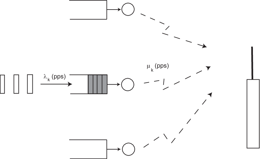
To keep the queue of user $k$ stable, we must have $\rho_{k}<1$ or $f(\gamma_{k})>\lambda_{k}\tau_{k}$. Now, let $W_{k}$ be a random variable representing the total packet delay for user $k$. This delay includes the time the packet spends in the queue, $W^{(q)}_{k}$, as well as the service time, $S_{k}$. Hence, we have

It is known that for an M/G/1 queue the average wait time (including the queuing and service time) is given by

where $\bar{L}_{k}=\rho_{k}+\frac{\rho_{k}^{2}+\lambda_{k}^{2}\sigma_{S_{k}}^{2}}{2(1-\rho_{k})}$ with $\sigma_{S_{k}}^{2}$ being the variance of the service time [25]. Therefore, the average packet delay for user $k$ is given by

We require the average packet delay for user $k$ to be less than or equal to $D_{k}$, i.e.,

This translates to

However, since $0\leq f(\gamma_{k})\leq 1$, we must have²² 2 Note that $f(\gamma)=1$ requires an infinite SIR which is not practical.

This means that $r_{k}=M\lambda_{k}$ and $D_{k}$ are feasible if only if they satisfy (11). Note that since the upper bound on the average delay cannot be smaller than the transmission time, i.e., $\frac{D_{k}}{\tau_{k}}\geq 1$, then we must have $R_{k}\geq M/D_{k}$. This automatically implies that $\lambda_{k}\tau_{k}+\frac{\tau_{k}}{D_{k}}-\frac{\lambda_{k}\tau_{k}^{2}}{2D_{k}}>0$.

Let us define $\eta_{k}=\lambda_{k}\tau_{k}+\frac{\tau_{k}}{D_{k}}-\frac{\lambda_{k}\tau_{k}^{2}}{2D_{k}}$. Then, (10) is equivalent to the condition $\gamma\geq\hat{\gamma}_{k}$ where

with $\eta_{k}<1$ and $R_{k}\geq M/D_{k}$. This means that the delay constraint in (9) translated into a lower bound on the output SIR.

Consider the non-cooperative joint power and rate control game (PRCG) $\mathcal{G}=[\mathcal{K},\{\mathcal{A}_{k}\},\{u_{k}\}]$ where $\mathcal{K}=\{1,2,\cdots,K\}$ is the set of users, $\mathcal{A}_{k}=[0,P_{max}]\times[0,B]$ is the strategy set for user $k$ with a strategy corresponding to a choice of transmit power and transmit rate, and $u_{k}$ is the utility function for user $k$. Here, $P_{max}$ and $B$ are the maximum transmit power and the system bandwidth, respectively. For the sake simplicity, throughout this paper, we assume $P_{max}$ is large. Each user chooses its transmit power and rate in order to maximize its own utility while satisfying its QoS requirements. The utility function for a user is defined as the ratio of the user’s goodput to its transmit power, i.e.,

where the goodput $T_{k}$ is the number of bits that is transmitted successfully per second and is given by

Therefore, the utility function for user $k$ is given by

This utility function, which was first introduced in [11, 12], has units of bits per joule and is particularly suitable for wireless networks where energy efficiency is important.

Fixing the other users’ transmit powers and rates, the utility-maximizing strategy for user $k$ is given by the solution of the following constrained maximization:

or equivalently

with $0\leq\eta_{k}<1$ where

and

Note that for a matched filter receiver and with random spreading sequences, the received SIR is approximately given by

where $h_{k}$ is the channel gain for user $k$ and $\sigma^{2}$ is the noise power in the bandwidth $B$.

Let us first look at the maximization in (17) without any constraints. Based on (20), we can write

Now, considering that $\tau_{k}=M/R_{k}$ must be less than or equal to $D_{k}$, the condition $0\leq\eta_{k}<1$ is equivalent to

Let us define

Note that for $R_{k}=\Omega_{k}^{\infty}$, we have $\eta_{k}=1$ and hence $\hat{\gamma}_{k}=\infty$. Also, define $\Omega_{k}^{*}$ as the rate for which $\hat{\gamma}_{k}=\gamma^{*}$, i.e.,

where $f^{*}=f(\gamma^{*})$. It is straightforward to show that $\hat{\gamma}_{k}$ is a decreasing function of $R_{k}$ for all $R_{k}\geq\Omega_{k}^{\infty}$. Therefore, $\hat{\gamma}_{k}>\gamma^{*}$ for all $\Omega_{k}^{\infty}\leq R_{k}<\Omega_{k}^{*}$. This means that user $k$ has no incentive to transmit at a rate smaller than $\Omega_{k}^{*}$. Furthermore, based on Proposition 1, any combination of $p_{k}$ and $R_{k}\geq\Omega_{k}^{*}$ which results in an output SIR equal to $\gamma^{*}$ is a solution to the constrained maximization in (17). Note that when $R_{k}=\Omega_{k}^{*}$ and $\gamma_{k}=\gamma^{*}$, we have $\bar{W}_{k}=D_{k}$.

If $\gamma^{*}$ is not feasible due to the maximum transmit power limitation, the user has to adjust its transmission rate and target SIR to satisfy its QoS constraints. In particular, user $k$ would choose $\tilde{\Omega}_{k}$ as its transmission rate such that its transmit rate and target SIR such that

where

This, of course, results in a reduction in the user’s energy efficiency.

For a non-cooperative game, a Nash equilibrium is defined as a set of strategies for which no user can unilaterally improve its own utility [26]. We saw in Section III that for our proposed non-cooperative game, each user has infinitely many strategies that maximize the user’s utility. In particular, any combination of $p_{k}$ and $R_{k}$ for which $\gamma_{k}=\gamma^{*}$ and $R_{k}\geq\Omega_{k}^{*}$ is a best-response strategy.

More generally, if we let $R_{k}=\tilde{R}_{k}\geq\Omega_{k}^{*}$ and provided that $\sum_{j=1}^{K}\frac{1}{1+\frac{B}{\tilde{R}_{j}\gamma^{*}}}<1$, then $(\tilde{p}_{k},\tilde{R}_{k})$ is a Nash equilibrium where $\tilde{p}_{k}=\frac{\sigma^{2}}{h_{k}}\left(\frac{\frac{1}{1+\frac{B}{\tilde{R}_{k}\gamma^{*}}}}{1-\sum_{j=1}^{K}\frac{1}{1+\frac{B}{\tilde{R}_{j}\gamma^{*}}}}\right)$.

Based on (15), at Nash equilibrium, the utility of user $k$ is given by

Therefore, the Nash equilibrium with the smallest $\tilde{R}_{k}$ achieves the largest utility. A higher transmission rate for a user requires a larger transmit power by that user to achieve $\gamma^{*}$. This not only reduces the user’s utility but also causes more interference for other users in the network and forces them to raise their transmit powers as well which will result in a reduction in their utilities. This means that the Nash equilibrium with $R_{k}=\Omega_{k}^{*}$ and $p_{k}^{*}$ for $k=1,\cdots,K$ is the Pareto-efficient Nash equilibrium.  ∎

We define the “size” of user $k$ as

Based on this definition, the feasibility condition $\sum_{k=1}^{K}\frac{1}{1+\frac{B}{\Omega_{k}^{*}\gamma^{*}}}<1$ can be written as

Note that the QoS requirements of user $k$ (i.e., its source rate $r_{k}$ and delay constraint $D_{k}$) uniquely determine $\Omega_{k}^{*}$ through (23) and, in turn, determine the size of the user (i.e., $\Phi_{k}^{*}$) through (25). The size of a user is basically an indication of the amount of network resources consumed by that user. A larger source rate or a tighter delay constraint for a user increases the size of the user. The network can accommodate a set of users if and only if their total size is less than 1. In Section VII, we use this framework to study the tradeoffs among throughput, delay, network capacity and energy efficiency.

In Section IV, we defined the “size” of a user based on its QoS requirements. Before joining the network, each user calculates its size using (25) and announces it to the access point. According to (26), the access point admits those users whose total size is less than 1. While the goal of each user is to maximize its own energy efficiency, a more sophisticated admission control can be performed to maximize the total network utility. In other words, out of the $K$ users, the access point can choose those users for which the total network utility is the largest, i.e.,

under the constraint that $\sum_{\ell\in{\mathcal{L}}}\Phi_{\ell}^{*}<1$.

Based on (24), the utility of user $\ell$ at the Pareto-dominant Nash equilibrium is given by

As a result, (27) becomes

or equivalently

under the constraint that $\sum_{\ell\in{\mathcal{L}}}\Phi_{\ell}^{*}<1$.

In general, obtaining a closed-form solution for (29) is difficult. Instead, in order to gain some insight, let us consider the special case in which all users are at the same distance from the access point. We first consider the scenario in which the users have identical QoS requirements (i.e., $\Phi_{1}^{*}=\cdots=\Phi_{K}^{*}=\Phi^{*}$). If we replace $\sum_{\ell=1}^{L}h_{\ell}$ by $L\mathbb{E}\{h\}$, then (29) becomes

Therefore, the optimal number of users for maximizing the total utility in the network is $L=\left[\frac{1}{2\Phi^{*}}\right]$ where $[x]$ represents the integer nearest to $x$.

Now consider another scenario in which there are $C$ classes of users. The users in class $c$ are assumed to all have the same QoS requirements and hence the same size, $\Phi^{*(c)}$. Since we are assuming that all the users have the same distance from the access point, they all have the same channel gains. Now, if the access point admits $L^{(c)}$ users from class $c$ then the total utility is given by

provided that $\sum_{c=1}^{C}L^{(c)}\Phi^{*(c)}<1$. Without loss of generality, let us assume that $\Phi^{*(1)}<\Phi^{*(2)}<\cdots<\Phi^{*(C)}$. It can be shown that $u_{T}$ is maximized when $L^{(1)}=\left[\frac{1}{2\Phi^{*(1)}}\right]$ with $L^{(c)}=0$ for $c=2,3,\cdots,C$. This is because adding a user from class 1 is always more beneficial in terms of increasing the total utility than adding a user from any other class. Therefore, in order to maximize the total utility in the network, the access point should admit only users from the class with the smallest size. While this solution maximizes the total network utility, it is not fair. A more sophisticated admission control mechanism can be used to improve the fairness.

In Section II, we defined the delay requirement of a user as an upper bound on the average total packet delay for that user where the total delay, $W_{k}$, is given by the sum of the queuing delay and service time. We have considered a scenario in which users choose their transmit powers and rates in a selfish and distributed manner such that they maximize their own energy efficiency while satisfying their delay requirements. In Section IV, we showed that at the Pareto-dominant Nash equilibrium, the transmit power and rate of a user are such that the delay bound is met with equality. However, it would be useful to obtain the delay profile of a user so that the deviations of the true delay from the average value can be quantified. More specifically, we would like to find a closed-form expression for $\textrm{Pr}\{W_{k}\leq c\}$ for all $c$.

To that end, let us define $w_{k}(t)$ as the probability density function (PDF) of $W_{k}$. Then, we have

Let $W_{k}^{*}(s)$ represent the Laplace transform for $w_{k}(t)$, i.e.,

It is known that for M/G/1 queues, we have

where $B_{k}^{*}(s)=\int_{0}^{\infty}e^{-st}b_{k}(t)\textrm{d}t$ with $b_{k}(t)$ being the PDF of the service time $S_{k}$ [25]. Based on (3), $b_{k}(t)$ is given by

where $\delta(\cdot)$ is the Dirac delta function. Therefore, we have

As a result,

However, obtaining a closed-form expression for $w_{k}(t)$ based on $W_{k}^{*}(s)$ in (36) is very difficult. But, recall from Section II that

Based on this we have

While finding the inverse Laplace transform of (37) is also difficult, we will shortly derive an accurate approximation for $w_{k}^{(q)}(t)$. Before doing that, let us first obtain the mean and variance of $W_{k}^{(q)}$ and $S_{k}$. For simplicity of notation, we will drop the subscript $k$ but it should be noted that all of our results are user dependent. Also, we replace $f(\gamma)$ by $f$.

Based on (3), the mean and variance of $S$ are, respectively, given by

and

From the known properties of M/G/1 queues [25], the mean and variance of $W^{(q)}$ are, respectively, given by

and

After some manipulations, it can be shown that the variance of $W^{(q)}$ is given by

To gain some insights into the contributions of the queuing delay and service time to the overall delay, let us define

and

Then, we have

and

At the Pareto-dominant Nash equilibrium, we have $\tau=\frac{M}{\Omega^{*}}$ and $\gamma=\gamma^{*}$. Therefore, based on (23), we have

Since $f^{*}$ is fixed and (44) only depends on the product $D\lambda$, then $\nu$ and $\chi$ also depend only on the product of $D$ and $\lambda$, not their individual values. Recall that $\lambda$ is the average source rate (in packets per second) and $D$ is the average delay bound. Together, they specify the QoS requirements of a user. Let $d=D\lambda$. So, for example, if the packet size $M$ is 100 bits, a source rate of $r=50$kbps results in $\lambda=500$pps. Then if the delay bound $D$ is 50ms, we have $d=25$. Fig. 2 shows the plots of $\nu$ and $\chi$ versus $d$ for $f(\gamma)=(1-e^{-\gamma})^{M}$.

Two important observations can be made from Fig. 2. First of all, for moderate and large values of $d$ (e.g., $d>10$), the average delay is dominated by the average wait time in the queue (i.e., $\bar{W}^{(q)})$. When $d$ is small, the average wait time in the queue and the average service time are comparable. For very small values of $d$, the service time dominates the total delay. Secondly, for most values of $d$ (i.e., $d>4$), the standard deviation of ${W}^{(q)}$ is at least ten times larger than that of $S$. This means that the variations in the total delay are caused mainly by the variations in $\bar{W}^{(q)}$. Therefore, in many cases, the variations in the total delay can be accurately approximated by the variations in the queuing delay.

Now let $w^{(q)}(t)$ be the PDF of the queuing delay. According to (37), the Laplace transform of $w^{(q)}(t)$ is given by

We can equivalently write $W^{(q)*}(s)$ as

where

and

Based on (45), we have

∎

As a result of Proposition 3, we have

Now if we restrict our attention to $0\leq t\leq t_{max}$ where $t_{max}>>D$, then we can approximate $p_{2}(t)$ numerically using the following:

or

Now, since the FFT of a discrete signal $z_{n}$ is given by

$p_{2}\left(\frac{t_{max}}{N}n\right)$ can be obtained by taking the IFFT of $\left(\frac{N}{t_{max}}\right)P_{2}(s)|_{s=i\frac{2\pi k}{100D}}$³³ 3 Since $p_{2}(t)$ is real, before taking the IFFT, we have to make sure that the samples of $P_{2}(s)$ satisfy the symmetry properties associated with the FFT of real signals.. In Section VII, we use this approximation along with (50) to obtain $w^{(q)}(t)$ and, consequently, approximate $\text{Pr}\{W^{(q)}\leq c\}$. This allows us to quantify the delay performance of the users at Nash equilibrium.

Let us consider the uplink of a DS-CDMA system with a total bandwidth of 5MHz (i.e. $B=5$MHz). A useful example for the efficiency function is ${f(\gamma)=(1-e^{-\gamma})^{M}}$. This serves as an approximation to the packet success rate that is very reasonable for moderate to large values of $M$. We use this efficiency function for our simulations. Using this, with $M=100$, we have $\gamma^{*}=6.48=8.1$dB. Each user in the network has a set of QoS requirements expressed as $(r_{k},D_{k})$ where $r_{k}$ is the source rate and $D_{k}$ is the delay requirement (upper bound on the average total delay) for user $k$. As explained in Section IV, the QoS parameters of a user define a “size” for that user, denoted by $\Phi_{k}^{*}$ given by (25). Before a user starts transmitting, it must announce its size to the access point. Based on the particular admission policy, the access point decides whether or not to admit the user. Throughout this section, we assume that the admitted users choose the transmit powers and rates that correspond to their Pareto-dominant Nash equilibrium.

Fig. 3 shows the user’s utility as a function of delay for different source rates. The total size of the other users in the network is assumed to be 0.2. The user’s utility is normalized by $Bh/\sigma^{2}$, and the delay is normalized by the inverse of the system bandwidth. As expected, a tighter delay requirement and/or a higher source rate results in a lower utility for the user.

Fig. 4 shows the user size, network capacity, transmission rate, and total goodput as a function of normalized delay for different source rates. The network capacity refers to the maximum number of users that can be admitted into the network assuming that all the users have the same QoS requirements (i.e., the same size). The transmission rate and goodput are normalized by the system bandwidth. The total goodput is obtained by multiplying the source rate by the total number of users. For example, a user with a source rate of 50 kbps and an average delay constraint of 50 ms (i.e., $r=50$ kbps and $D=50$ ms) has a size equal to 0.072. As the QoS requirements become more stringent (i.e., a higher source rate and/or a smaller delay), the size of the user increases which means more network resources are required to accommodate the user. This results in a reduction in the network capacity. For $r=50$ kbps and $D=50$ ms, the transmission rate is equal to 59.65 kbps, the network capacity is equal to 13, and the total goodput is 650 kbps. It is also observed from the figure that when the delay constraint is loose, the total goodput is almost independent of the source rate. This is because a lower source rate is compensated by the fact that more users can be admitted into the network. On the other hand, when the delay constraint in tight, the total goodput is higher for larger source rates.

Now, to study admission control, let us consider a network with three different classes of users/sources:

1. 1.

   Class $A$ users for which $r^{(A)}=5$ kbps and $D^{(A)}=10$ ms.

2. 2.

   Class $B$ users for which $r^{(B)}=50$ kbps and $D^{(B)}=50$ ms.

3. 3.

   Class $C$ users for which $r^{(C)}=150$ kbps and $D^{(C)}=1000$ ms.

We can calculate the size of a user in each class using (25) to get $\Phi^{*^{(A)}}=0.0198$, $\Phi^{*^{(B)}}=0.0718$, and $\Phi^{*^{(C)}}=0.1848$. This means that users in classes $B$ and $C$ respectively consume approximately 3.6 and 9.3 times as much resources as a user in class $A$.

For the purpose of illustration and to keep the comparison fair, let us assume that there are a large number of users in each class and that they all are at the same distance from the access point (i.e., they all have the same average channel gain). The access point receives requests from the users and has to decide which ones to admit in order to maximize the total utility in the network (see (29)). We know from Section V that since users in class $A$ have the smallest size, the total utility is maximized if the access point picks users from class $A$ only with $L^{(A)}=\left[1/2\Phi^{*^{(}A)}\right]=25$. However, this solution does not take into account fairness. Instead, we may be more interested in cases where more than one class of users are admitted. Table I shows the percentage loss in the total utility (energy efficiency) for several choices of $L^{(A)},L^{(B)}$ and $L^{(C)}$. It is observed that admitting “large” users into the network results in significant reductions in the energy efficiency and capacity of the network.

Let us now focus on the delay profile of a user in class $B$. For this user, we have $r^{(B)}=50$ kbps (or $\lambda^{(B)}=500$ pps) and $D^{(B)}=50$ ms. Therefore, $d^{(B)}=25$. From (38)–(41), we have $\bar{S}^{(B)}=2$ ms, $\sigma_{S}^{(B)}=0.74$ ms, $\bar{W}^{(q)(B)}=48$ ms and $\sigma_{W^{(q)}}^{(B)}=48$ ms. It is clear that for this user the queuing delay is the dominant component of the total delay. This can also be seen from Fig. 2. Therefore, the cumulative distribution function (CDF) of $W^{(B)}$, i.e., $\text{Pr}\{W^{(B)}\leq t\}$, can be very accurately approximated by the CDF of $W^{(q)(B)}$. Hence, we can use (50) to numerically compute the CDF of the queuing delay. This CDF is plotted in Fig. 5. It is seen from the figure that about 63% of the time, the delay experienced by a packet is less than the average delay bound and 85% of the time, the delay is less than twice the average delay.

We have studied the cross-layer problem of QoS-constrained power and rate control in wireless networks using a game-theoretic framework. We have proposed a non-cooperative game in which users seek to choose their transmit powers and rates in such a way as to maximize their utilities and at the same time satisfy their QoS requirements. The utility function considered here measures the number of reliable bits transmitted per joule of energy consumed. The QoS requirements for a user consist of the average source rate and an upper bound on the average delay where the delay includes both transmission and queuing delays. We have derived the Nash equilibrium solution for the proposed game and obtained a closed-form solution for the user’s utility at equilibrium. Using this framework, we have studied the tradeoffs among throughput, delay, network capacity and energy efficiency, and have shown that the presence of users with stringent QoS requirements results in significant reductions in network capacity and energy efficiency. The delay performance of users at Nash equilibrium are also analyzed.

References

- [1] M. L. Honig and J. B. Kim, “Allocation of DS-CDMA parameters to achieve multiple rates and qualities of service,” Proceedings of the IEEE Global Telecommunications Conference (Globecom), pp. 1974–1978, London, UK, November 1996.
- [2] S.-J. Oh and K. M. Wasserman, “Adaptive resource allocation in power constrained CDMA mobile networks,” Proceedings of the IEEE Wireless Communications and Networking Conference (WCNC), pp. 510–514, New Orleans, LA, September 1999.
- [3] B. Collins and R. Cruz, “Transmission policies for time varying channels with average delay constraints,” Proceedings of the 37th Annual Allerton Conference on Communication, Control, and Computing, Monticello, IL, October 1999.
- [4] B. Prabhakar, E. Uysal-Biyikoglu, and A. El Gamal, “Energy-efficient transmission over a wireless link via lazy packet scheduling,” Proceedings of 20th Annual Joint Conference of the IEEE Computer and Communications Societies (INFOCOM), Anchorage, AK, April 2001.
- [5] R. A. Berry and R. G. Gallager, “Communication over fading channels with delay constraints,” IEEE Transactions on Information Theory, vol. 48, pp. 1135–1149, May 2002.
- [6] A. Fu, E. Modiano, and J. Tsitsiklis, “Optimal energy allocation for delay-constrained data transmission over a time-varying channel,” Proceedings of 22nd Annual Joint Conference of the IEEE Computer and Communications Societies (INFOCOM), pp. 1095–1105, San Francisco, CA, March/April 2003.
- [7] E. Uysal-Biyikoglu and A. El Gamal, “Energy-efficient packet transmission over a multiaccess channel,” Proceedings of IEEE International Symposium on Information Theory (ISIT), p. 153, Lausanne, Switzerland, June/July 2002.
- [8] T. P. Coleman and M. Médard, “A distributed scheme for achieving energy-delay tradeoffs with multiple service classes over a dynamically varying network,” IEEE Journal on Selected Areas in Communications (JSAC), vol. 22, pp. 929–941, June 2004.
- [9] N. Ahmed, M. A. Khojestapour, and R. G. Baraniuk, “Delay-limited throughput maximization for fading channels using rate and power control,” Proceedings of the IEEE Global Telecommunications Conference (Globecom), pp. 3459–3463, Dallas, TX, November/December 2004.
- [10] H. Ji and C.-Y. Huang, “Non-cooperative uplink power control in cellular radio systems,” Wireless Networks, vol. 4, pp. 233–240, April 1998.
- [11] V. Shah, N. B. Mandayam, and D. J. Goodman, “Power control for wireless data based on utility and pricing,” Proceedings of the 9th IEEE International Symposium on Personal, Indoor, and Mobile Radio Communications (PIMRC), pp. 1427–1432, Boston, MA, September 1998.
- [12] D. J. Goodman and N. B. Mandayam, “Power control for wireless data,” IEEE Personal Communications, vol. 7, pp. 48–54, April 2000.
- [13] M. Xiao, N. B. Shroff, and E. K. P. Chong, “A utility-based power-control scheme in wireless cellular systems,” IEEE/ACM Transactions on Networking, vol. 11, pp. 210–221, April 2003.
- [14] C. Zhou, M. L. Honig, and S. Jordan, “Two-cell power allocation for downlink cdma,” IEEE Transactions on Wireless Communications, vol. 5, pp. 2256–2266, November 2004.
- [15] T. Alpcan, T. Basar, R. Srikant, and E. Altman, “CDMA uplink power control as a noncooperative game,” Wireless Networks, vol. 8, pp. 659–669, November 2002.
- [16] N. Feng, S.-C. Mau, and N. B. Mandayam, “Pricing and power control for joint network-centric and user-centric radio resource management,” IEEE Transactions on Communications, vol. 52, pp. 1547–1557, September 2004.
- [17] C. W. Sung and W. S. Wong, “A noncooperative power control game for multirate CDMA data networks,” IEEE Transactions on Wireless Communications, vol. 2, pp. 186–194, January 2003.
- [18] C. U. Saraydar, N. B. Mandayam, and D. J. Goodman, “Pricing and power control in a multicell wireless data network,” IEEE Journal on Selected Areas in Communications (JSAC), vol. 19, pp. 1883–1892, October 2001.
- [19] C. U. Saraydar, N. B. Mandayam, and D. J. Goodman, “Efficient power control via pricing in wireless data networks,” IEEE Transactions on Communications, vol. 50, pp. 291–303, February 2002.
- [20] S. Gunturi and F. Paganini, “Game theoretic approach to power control in cellular CDMA,” Proceedings of the 58th IEEE Vehicular Technology Conference (VTC), pp. 2362–2366, Orlando, FL, October 2003.
- [21] E. Altman and Z. Altman, “S-modular games and power control in wireless networks,” IEEE Transactions on Automatic Control, vol. 48, pp. 839–842, May 2003.
- [22] F. Meshkati, H. V. Poor, S. C. Schwartz, and N. B. Mandayam, “An energy-efficient approach to power control and receiver design in wireless data networks,” IEEE Transactions on Communications, vol. 52, pp. 1885–1894, November 2005.
- [23] F. Meshkati, M. Chiang, H. V. Poor, and S. C. Schwartz, “A game-theoretic approach to energy-efficient power control in multicarrier CDMA systems,” IEEE Journal on Selected Areas in Communications (JSAC), vol. 24, pp. 1115–1129, June 2006.
- [24] F. Meshkati, H. V. Poor, and S. C. Schwartz, “A non-cooperative power control game in delay-constrained multiple-access networks,” Proceedings of the IEEE International Symposium on Information Theory (ISIT), pp. 700–704, Adelaide, Australia, September 2005.
- [25] D. Gross and C. M. Harris, Fundamentals of Queueing Theory. John Wiley & Sons, New York, 1985.
- [26] D. Fudenberg and J. Tirole, Game Theory. MIT Press, Cambridge, MA, 1991.
- [27] A. D. Wunsch, Complex Variables with Applications. Addison-Wesley Publishing Company, Reading, MA, 1994.
- [28] I. M. Ryshik and I. S. Gradstein, Tables of Series, Products, and Integrals. Veb Deutscher Verlag der Wissenschaften, Berlin, 1963.