Relativistic diffusion equation from stochastic quantization

P.O. Kazinski Email: kpo@phys.tsu.ru Affiliation: Department of Physics, Tomsk State University, Tomsk, 634050 Russia

August 11, 2026

Abstract

The new scheme of stochastic quantization is proposed. This quantization procedure is equivalent to the deformation of an algebra of observables in the manner of deformation quantization with an imaginary deformation parameter (the Planck constant). We apply this method to the models of nonrelativistic and relativistic particles interacting with an electromagnetic field. In the first case we establish the equivalence of such a quantization to the Fokker-Planck equation with a special force. The application of the proposed quantization procedure to the model of a relativistic particle results in a relativistic generalization of the Fokker-Planck equation in the coordinate space, which in the absence of the electromagnetic field reduces to the relativistic diffusion (heat) equation. The stationary probability distribution functions for a stochastically quantized particle diffusing under a barrier and a particle in the potential of a harmonic oscillator are derived.

pacs

05.40.-a

I Introduction

There are many different approaches to stochastic quantization and in understanding what it is (see for the review Nam). In this paper we propose another procedure of stochastic quantization, which in some sense generalizes the operator approach to the Fokker-Planck equation used in Nam; Par; Ris; ZJ. This new method of quantization gives a stochastic mechanics, which is not equivalent to quantum mechanics both in the manner of Nelson’s stochastic quantization Nel, and the Parisi-Wu stochastic quantization in the fictitious time. Rather we interpret the stochastic quantization from the point of view of the deformation quantization BFFLS, i.e., as a deformation of an associative algebra of observables (smooth functions over a symplectic manifold) with an imaginary deformation parameter as opposed to an ordinary quantum mechanics with a real deformation parameter (the Planck constant). This formulation of stochastic quantization allows us to apply the developed methods of quantum mechanics to the stochastic mechanics almost without any changing.

In this paper we only formulate the general notions of such a stochastic quantization and show how it works on simple examples: the models of relativistic and nonrelativistic particles interacting with an electromagnetic field. The development of the secondary stochastic quantization and its applications to the models with infinite degrees of freedom are left for a future work.

The paper is organized as follows. In the section II we specify the rules of stochastic quantization and introduce basic notions of the proposed stochastic mechanics. In the section III we consider two examples: the stochastically quantized models of a nonrelativistic particle in the subsection III.1 and a relativistic particle in the subsection III.2.

As far as the nonrelativistic case is concerned we find several simple stationary solutions to the derived equations of motion: a particle diffuses a potential barrier and a particle in the potential of a harmonic oscillator. Here we also obtain the functional integral representation for a transition probability and the explicit formula for a first correction to the Newton equations due to the diffusion process. Besides we establish that the proposed stochastic mechanics can be reproduced by an appropriate Langevin equation.

In the relativistic case we obtain a Lorentz-invariant generalization of the Fokker-Planck equation in the coordinate space, which in the absent of the electromagnetic fields reduces to the relativistic diffusion (heat) equation (see for the review JosPre). By this example we also show how the basic concepts of the BRST-quantization (see, e.g., HeTe) look in the context of stochastic mechanics.

In conclusion we sum up the results of the paper and outline the prospects for possible further research.

II The rules of stochastic quantization

In this section we formulate the rules of stochastic quantization and define the main concepts of such a stochastic mechanics.

Let us given a classical system with the Hamilton function $H(t,x,p)$ , where $x^{i}$ and $p_{j}$ are canonically conjugated with respect to the Poisson bracket positions and momenta

\{x^{i},p_{j}\}=\delta^{i}_{j},\qquad i,j=\overline{1,d},

(1)

where $d$ is a dimension of the configuration space. As in quantum mechanics we associate with such a system the Hilbert space of all the square-integrable functions depending on $x$ with the standard inner product

\langle\psi|\varphi\rangle=\int d^{d}x\psi^{*}(x)\varphi(x),

(2)

Henceforth unless otherwise stated we consider only real-valued functions in this space.

In the Hilbert space we define the operators $\hat{x}^{i}$ and $\hat{p}_{j}$ such that

[\hat{x}^{i},\hat{p}_{j}]=\hbar\delta^{i}_{j},\qquad\hat{x}^{i+}=\hat{x}^{i},\qquad\hat{p}_{j}^{+}=-\hat{p}_{j},

(3)

where $\hbar$ is a small positive number and the cross denotes the conjugation with respect to the inner product (2). Define the Hamiltonian $\hat{H}(t,\hat{x},\hat{p})$ by the von Neumann corresponding rules¹¹ 1 We emphasize that contrary to Nam the Hamiltonian $H(t,x,p)$ is not the Fokker-Planck Hamiltonian.

x^{i}\rightarrow\hat{x}^{i},\qquad p_{j}\rightarrow\hat{p}_{j}.

(4)

The state of the stochastic system is characterized by two vectors $|\psi\rangle$ and $|O\rangle$ from the Hilbert space with the evolution

\hbar\frac{d}{dt}|\psi\rangle=\hat{H}|\psi\rangle,\qquad\hbar\frac{d}{dt}\langle O|=-\langle O|\hat{H},

(5)

and the normalization condition

\langle O|\psi\rangle=1.

(6)

Define an average of the physical observable $T(t,x,p)$ by the matrix element

\langle\hat{T}\rangle\equiv\langle O|\hat{T}(t,\hat{x},\hat{p})|\psi\rangle,

(7)

where the operator $\hat{T}(t,\hat{x},\hat{p})$ is constructed from $T(t,x,p)$ by the corresponding rules (4). Then the Heisenberg equations for averages are

\hbar\frac{d}{dt}\langle\hat{T}\rangle=\langle\partial_{t}\hat{T}+[\hat{T},\hat{H}]\rangle.

(8)

By definition the probability density function is

\rho(x)=\langle O|x\rangle\langle x|\psi\rangle,

(9)

where $|x\rangle$ are the eigenvectors for the position operators corresponding to the eigenvalue $x$ . The transition probability from the position $x$ at the time $t$ to $x^{\prime}$ at the time $t^{\prime}$ looks like

G(t^{\prime},x^{\prime};t,x)=\langle O(t^{\prime})|x^{\prime}\rangle\langle x^{\prime}|\hat{U}_{t^{\prime},t}|x\rangle\frac{1}{\langle O(t)|x\rangle},

(10)

where $\hat{U}_{t^{\prime},t}$ is the evolution operator obeying the equations

\hbar\partial_{t^{\prime}}\hat{U}_{t^{\prime},t}=\hat{H}\hat{U}_{t^{\prime},t},\qquad\hat{U}_{t,t}=\hat{1}.

(11)

The transition probability (10) possesses the property of a Markov process

G(t^{\prime},x^{\prime};t,x)=\int d^{d}yG(t^{\prime},x^{\prime};\tau,y)G(\tau,y;t,x).

(12)

By the standard means (see, e.g., Wein) we can construct a path integral representation of the transition probability (10). To this end we introduce auxiliary vectors $|ip\rangle$ in the Hilbert space such that

\hat{p}_{j}|ip\rangle=ip_{j}|ip\rangle,\qquad\langle ip^{\prime}|ip\rangle=\delta^{d}(p-p^{\prime}),\qquad\int\frac{d^{d}p}{(2\pi\hbar)^{d}}|ip\rangle\langle ip|=\hat{1}.

(13)

In the coordinate representation we have

\langle x|ip\rangle=\exp{\{-\frac{i}{\hbar}p_{i}x^{i}\}}.

(14)

Then inserting the unity partition (13) into the transition probability (10) we arrive at

\langle O(t+dt)|x^{\prime}\rangle\langle x^{\prime}|\hat{U}_{t+dt,t}|x\rangle\frac{1}{\langle O(t)|x\rangle}=\\ \langle x^{\prime}|\exp\left\{\frac{dt}{\hbar}\left[\hat{H}(t,\hat{x},\hat{p}+\hbar\nabla\ln O(t,\hat{x}))+\hbar\partial_{t}\ln O(t,\hat{x})\right]\right\}|x\rangle=\\ \int\frac{d^{d}p(t)}{(2\pi\hbar)^{d}}\exp{\left\{-\frac{i}{\hbar}\left[p_{i}(t)\dot{x}^{i}(t)+i\left(\bar{H}(t,x(t+dt),ip(t))+\hbar\partial_{t}\ln O(t,x(t))\right)\right]dt\right\}},

(15)

where $x(t)=x$ , $x(t+dt)=x^{\prime}$ , $\dot{x}(t)=(x(t+dt)-x(t))/dt$ , $O(t,x)=\langle O(t)|x\rangle$ and

\bar{H}(t,x,ip)=\langle x|\hat{H}(t,\hat{p}+\hbar\nabla\ln O(t,\hat{x}),\hat{x})|ip\rangle\langle ip|x\rangle

(16)

is a $qp$ -symbol of the Hamiltonian $\hat{H}$ with the momentum $\hat{p}+\hbar\nabla\ln\hat{O}$ .

The functional integral representation of the transition probability is obtained by the repeatedly use of the property (12) and the formula (15):

G(t^{\prime},x^{\prime};t,x)=\int\prod_{\tau\in(t,t^{\prime})}d^{d}x(\tau)\prod_{\tau\in[t,t^{\prime})}\frac{d^{d}p(\tau)}{(2\pi\hbar)^{d}}\times\\ \exp\left\{-\frac{i}{\hbar}\int\limits_{t}^{t^{\prime}-d\tau}d\tau\left[p_{i}(\tau)\dot{x}^{i}(\tau)+i\left(\bar{H}(\tau,x(\tau+d\tau),ip(\tau))+\hbar\partial_{\tau}\ln O(\tau,x(\tau))\right)\right]\right\}.

(17)

The property (12) guarantees that the functional integral representation (17) does not depend on what slices the time interval $[t,t^{\prime}]$ is cut (for more details see, e.g., DemCh).

To conclude this section we formulate the above stochastic mechanics in terms of the density operator

\hat{\rho}=|\psi\rangle\langle O|.

(18)

From (5) and (6) it follows that

\hbar\frac{d}{dt}\hat{\rho}=[\hat{H},\hat{\rho}],\qquad\Sp\hat{\rho}=1.

(19)

The averages are calculated as in quantum mechanics

\langle\hat{T}\rangle=\Sp(\hat{\rho}\hat{T}).

(20)

The probability density function $\rho(t,x)$ is the average of the projector $|x\rangle\langle x|$ and obeys the evolution law

\hbar\partial_{t}\rho(t,x)=\langle x|[\hat{H},\hat{\rho}]|x\rangle.

(21)

As we will see in the next section this equation is nothing but the Fokker-Planck equation. Notice that from the definition (18) the density operator is idempotent, i.e.,

\hat{\rho}^{2}=\hat{\rho}.

(22)

By analogy with quantum mechanics one can say that such a density operator describes a pure state. The transition probability (10) is

G(t^{\prime},x^{\prime};t,x)=\Sp(\hat{\rho}(t^{\prime},t)|x^{\prime}\rangle\langle x^{\prime}|),\qquad\hat{\rho}(t,t)=\frac{|x\rangle\langle O|}{\langle O|x\rangle},

(23)

where $\hat{\rho}(t^{\prime},t)$ obeys the von Neumann equation (19).

The formulation of the stochastic mechanics in terms of the density operator reveals that from the mathematical point of view the positions $x^{i}$ are not distinguished over the momenta $p_{j}$ as it seems from (3). The above stochastic quantization can be considered as a formal deformation of the algebra of classical observables in the manner of deformation quantization BFFLS. For a linear symplectic space the Moyal product is

f(z)*g(z)=\sum\limits_{n=0}^{\infty}\frac{1}{n!}\left(\frac{\hbar}{2}\right)^{n}\omega^{a_{1}b_{1}}\ldots\omega^{a_{n}b_{n}}\partial_{a_{1}\ldots a_{n}}f(z)\partial_{b_{1}\ldots b_{n}}g(z),

(24)

where $z\equiv(x,p)$ , $a_{n},b_{n}=\overline{1,2d}$ , $f(z)$ and $g(z)$ are the Weil symbols, and $\omega^{ab}$ is the inverse to the symplectic $2$ -form $\omega_{ab}$ . The trace formula for averages is given by

\langle\hat{T}\rangle=\Sp(\hat{\rho}\hat{T})=\int\frac{d^{d}xd^{d}p}{(2\pi\hbar)^{d}}\sqrt{\det{\omega_{ab}}}\rho(x,p)T(p,x),

(25)

where $\rho(x,p)$ and $T(p,x)$ are $qp$ - and $pq$ -symbols of the corresponding operators. For instance, the $qp$ -symbol of the density operator is

\rho(x,ip)=\langle x|\hat{\rho}|ip\rangle\langle ip|x\rangle.

(26)

Thus all the general results regarding deformation quantization of symplectic Fed and Poisson Kont manifolds, quantization of systems with constraints (see, e.g., HeTe) etc. are valid in such a stochastic mechanics.

III Examples

III.1 Nonrelativistic particle

In this subsection we consider the stochastic quantization of the model of a nonrelativistic particle and in particular establish the one-to-one correspondence of such a quantized model with appropriate Langevin and Fokker-Planck equations.

According to the general rules expounded in the previous section the Hamiltonian for a nonrelativistic particle looks like²² 2 We use the Minkowski metric $\eta_{\mu\nu}=diag(-1,1,1,1)$ and the system of units in which the velocity of light $c=1$ . The bold face is used for the spacial components of $4$ -vectors.

\hat{H}=\frac{(\hat{\mathbf{p}}-\hat{\mathbf{A}})^{2}}{2m}+\hat{A}^{0},

(27)

and the evolution equations (5) in the coordinate representation are

\hbar\partial_{t}\psi(t,x)=\left[\frac{(\hat{\mathbf{p}}-\mathbf{A})^{2}}{2m}-A_{0}\right]\psi(t,x),\qquad\hbar\partial_{t}O(t,x)=-\left[\frac{(\hat{\mathbf{p}}+\mathbf{A})^{2}}{2m}-A_{0}\right]O(t,x),

(28)

where $\hat{\mathbf{p}}=-\hbar\nabla$ and $A_{\mu}(t,x)$ are gauge fields, which we will call the electromagnetic fields. The physical meaning of the fields $A_{\mu}$ will be elucidated by the Fokker-Planck equation associated with (28).

The equations (28) are invariant under the following gauge transformations

\psi(t,x)\rightarrow\psi(t,x)e^{-\varphi(t,x)},\qquad O(t,x)\rightarrow O(t,x)e^{\varphi(t,x)},\qquad A_{\mu}(t,x)\rightarrow A_{\mu}(t,x)+\partial_{\mu}\varphi(t,x).

(29)

In particular, these transformations do not change the probability density function. The conserved $4$ -current corresponding to the gauge transformations (29) is

j^{\mu}=\left(O\psi,\frac{1}{2m}\left[O(\hat{\mathbf{p}}-\mathbf{A})\psi-\psi(\hat{\mathbf{p}}+\mathbf{A})O\right]\right).

(30)

The system (28) is Lagrangian with the Hamiltonian action of the form

S_{H}[O,\psi]=\int dtd^{d}x\left\{\hbar O\partial_{t}\psi-O\left[\frac{(\hat{\mathbf{p}}-\mathbf{A})^{2}}{2m}-A_{0}\right]\psi\right\},

(31)

that is the fields $\psi(t,x)$ and $O(t,x)$ are canonically conjugated.

With the identification

O(t,x)\equiv e^{\frac{1}{\hbar}S(t,x)},\qquad\psi(t,x)\equiv\rho(t,x)e^{-\frac{1}{\hbar}S(t,x)},

(32)

the system of evolutionary equations (28) becomes³³ 3 For possible nonlinear generalizations see, e.g., Scar.

\partial_{t}\rho=-\Div\left[-\frac{\hbar}{2m}\nabla\rho+\frac{\nabla S-\mathbf{A}}{m}\rho\right],\qquad\partial_{t}S-A_{0}+\frac{(\nabla S-\mathbf{A})^{2}}{2m}=-\frac{\hbar}{2m}\Div(\nabla S-\mathbf{A}).

(33)

The first equation in this system is the Fokker-Planck equation, while the second equation can be referred to as the quantum Hamilton-Jacobi equation LMSh.

Now it is evident that if one neglects quantum corrections then the initially $\delta$ -shaped probability density function $\rho(t,x)$ keeps its own form and propagates as a classical charged particle in the electromagnetic fields⁴⁴ 4 Such an interpretation for the Langevin equation with a non-conservative force was proposed in LepMa. with particle’s momentum $\nabla S(t,x)-\mathbf{A}(t,x)$ .

Let us find the evolution of the average position of the stochastically quantized particle. The Heisenberg equations (8) for this model are

m\frac{d}{dt}\langle\mathbf{x}\rangle=\langle\hat{\mathbf{p}}-\mathbf{A}\rangle=\langle\nabla S-\mathbf{A}\rangle,\qquad m\frac{d^{2}}{dt^{2}}\langle\mathbf{x}\rangle=\langle\mathbf{E}\rangle+\frac{1}{m}\langle(\nabla S-\mathbf{A})\times\mathbf{H}\rangle+\frac{\hbar}{2m}\langle\Rot{\mathbf{H}}\rangle.

(34)

In the case that $\rho(t,x)$ is sufficiently localized comparing to the characteristic scale of variations of the electromagnetic fields the angle brackets can be carried through the electromagnetic fields to obtain a closed system of evolutionary equations on the average position. They are simply the Newton equations with the “quantum” correction.

Notice that the analog of the quantum mechanical uncertainty relation is

\langle(x^{i})^{2}\rangle\langle(p^{i}_{os})^{2}\rangle\geq\frac{\hbar^{2}}{4},

(35)

where $\mathbf{p}_{os}=-\hbar\nabla\ln\rho^{1/2}$ is the osmotic momentum. It is easily proven from the inequality

\int d^{d}x\left[(\xi x^{i}-\hbar\partial_{i})\rho^{1/2}\right]^{2}\geq 0,\quad\forall\,\xi\in\mathbb{R}.

(36)

The equipartition law UlhOrn can be discovered from

\lim_{dt\rightarrow 0}T\{\frac{m\dot{\hat{\mathbf{x}}}^{2}(t)}{2}dt\}=\frac{m}{2\hbar}[\hat{\mathbf{x}},[\hat{\mathbf{x}},\hat{H}]]=\frac{\hbar}{2}d,

(37)

where $\hat{\mathbf{x}}(t)$ are the position operators in the Heisenberg representation and $T$ means the chronological ordering.

To reproduce the Fokker-Planck equation associated with the Langevin equation of the form (see, e.g., ZJ)

\frac{d}{dt}x^{i}(t)=f^{i}(t,x(t))+\nu^{i}(t),\qquad\langle\nu^{i}(t)\rangle=0,\qquad\langle\nu^{i}(t)\nu^{j}(t^{\prime})\rangle=\hbar\delta^{ij}\delta(t-t^{\prime}),

(38)

where $\nu^{i}(t)$ is a Gaussian white noise, one has to solve the system of equations ( $m=1$ )

\nabla S(t,x)-\mathbf{A}(t,x)=\mathbf{f}(t,x),\qquad A_{0}-\partial_{t}S=\frac{1}{2}\left(\mathbf{f}^{2}+\hbar\Div\mathbf{f}\right),

(39)

with respect to $A_{\mu}(t,x)$ and $S(t,x)$ . Obviously, this system admits a solution. The arbitrariness in the definition of $A_{\mu}(t,x)$ and $S(t,x)$ from the equations (39) is equivalent to the arbitrariness of a gauge. The converse is also true, i.e., for any given solution $S(t,x)$ and $A_{\mu}(t,x)$ of the quantum Hamilton-Jacobi equation (33) we can construct the force $\mathbf{f}(t,x)$ in the Langevin equation by the formula (39), which gives rise to the same probability distribution function. The equations (34) for the average position of the particle in the representation (39) become

\frac{d}{dt}\langle\mathbf{x}\rangle=\langle\mathbf{f}\rangle,\qquad\frac{d^{2}}{dt^{2}}\langle\mathbf{x}\rangle=\langle(\partial_{t}+(\mathbf{f}\nabla))\mathbf{f}\rangle+\frac{\hbar}{2}\langle\triangle\mathbf{f}\rangle.

(40)

To gain a better physical insight into the stochastically quantized model of a nonrelativistic particle we construct the functional integral representation (17) of the transition probability. The $qp$ -symbol of the operator appearing in the formula (16) is

\bar{H}(t,x,ip)=\frac{1}{2m}\left[-\mathbf{p}^{2}+2i\mathbf{p}(\nabla S-\mathbf{A})-\hbar\Div(\nabla S-\mathbf{A})\right]+A^{0}.

(41)

Substituting this expression into (17) and integrating over momenta we arrive at

G(t^{\prime},x^{\prime};t,x)=\int\left(\frac{m}{2\pi\hbar d\tau}\right)^{d/2}\prod_{\tau\in(t,t^{\prime})}\left(\frac{m}{2\pi\hbar d\tau}\right)^{d/2}d^{d}x(\tau)\times\\ \exp\left\{-\frac{1}{\hbar}\int\limits_{t}^{t^{\prime}-d\tau}d\tau\left[\frac{m}{2}\dot{\mathbf{x}}^{2}+(\mathbf{A}-\nabla S)\dot{\mathbf{x}}-(A^{0}+\partial_{\tau}S)-\frac{\hbar}{2m}\Div(\mathbf{A}-\nabla S)\right]\right\},

(42)

where the functions $A_{\mu}(t,x)$ and $S(t,x)$ obey the quantum Hamilton-Jacobi equation (33) and are taken at the point $(t,x)=(\tau,x(\tau+d\tau))$ . Now it is obvious that the main contribution to the transition probability is made by the paths approximating a classical trajectory. In the representation (39) the transition probability (42) reduces to the well known result

G(t^{\prime},x^{\prime};t,x)=\int\frac{1}{(2\pi\hbar d\tau)^{d/2}}\prod_{\tau\in(t,t^{\prime})}\frac{d^{d}x(\tau)}{(2\pi\hbar d\tau)^{d/2}}\times\\ \exp\left\{-\frac{1}{\hbar}\int\limits_{t}^{t^{\prime}-d\tau}d\tau\left[\frac{(\dot{\mathbf{x}}(\tau)-\mathbf{f}(\tau,x(\tau+d\tau)))^{2}}{2}+\hbar\Div\mathbf{f}(\tau,x(\tau+d\tau))\right]\right\}.

(43)

Usually the force $\mathbf{f}(t,x)$ is specified so that the corresponding Fokker-Planck equation admits a Boltzmann’s type stationary solution. As one can see from the equations (33) that is the case if $\nabla S$ and $A_{\mu}$ are of the order of $\hbar$ or higher, i.e., the momentum and energy of the particle are small. For example, the Boltzmann distribution

\rho(x)=e^{-U(x)}/Z,

(44)

where $U(x)$ is some time-independent potential function measured in terms of the temperature, is reproduced by the following solution to (33)

S=-\frac{\hbar U}{2},\qquad A_{0}=\frac{\hbar^{2}}{4}\left[\frac{1}{2}(\nabla U)^{2}+\Delta U\right],\qquad\mathbf{A}=0.

(45)

Possibly such “quantum” corrections to the electromagnetic potential naturally arise from the stochastic quantization of the electromagnetic fields (we leave a verification of this supposition for future investigations). Nevertheless in a high-energy limit, while the diffusion results in small corrections to the dynamics, the gauge fields $A_{\mu}$ in the equations (33) can be interpreted as the electromagnetic fields. Notice that under this interpretation the equations (33) are Galilean invariant as opposed to the case, when $\nabla S-\mathbf{A}$ is a force.

To conclude this section we give several simple one-dimensional stationary solutions to the equations (33).

The stationary solutions for $A_{\mu}=0$ . The system of equations (33) is

\hbar\rho^{\prime}=2S^{\prime}\rho,\qquad\hbar S^{\prime\prime}+S^{\prime 2}=2mE,

(46)

where $E$ is a constant. The solutions are

$\displaystyle E$	$\displaystyle=\frac{p^{2}}{2m}>0,$	$\displaystyle\quad\rho$	$\displaystyle=c_{1}e^{-2px/\hbar}+c_{2}e^{2px/\hbar}+2\sqrt{c_{1}c_{2}},$	(47)
$\displaystyle E$	$\displaystyle=0,$	$\displaystyle\quad\rho$	$\displaystyle=(x-c)^{2}/Z,\quad\text{or}\quad\rho=c,$
$\displaystyle E$	$\displaystyle<0,$	$\displaystyle\quad\rho$	$\displaystyle=\frac{1}{Z}\cos^{2}\left[\frac{\sqrt{2m\|E\|}}{\hbar}(x-c)\right].$

In the last case we can take only one hump of the squared cosine function and then continue the solution by zero on the residual part of the line.

To obtain solutions with a finite norm describing a diffusion of particles under a potential barrier we just have to join the solutions in (47). For a potential barrier of the form⁵⁵ 5 For brevity, we hereinafter designate only nonvanishing parts of a piecewise function. All the below solutions have a continuous first derivative on a whole real line.

A^{0}(x)=V,\quad x\geq 0,

(48)

where $V$ is a positive constant, we have

\rho=\frac{1}{Z}\left\{\begin{array}[]{ll}e^{2px/\hbar}(1+p^{2}l_{p}^{2}\hbar^{-2})^{-1},&x<0;\\ \cos^{2}\{[x-l_{p}\arctan(pl_{p}\hbar^{-1})]/l_{p}\},&0\leq x<l_{p}[\arctan(pl_{p}\hbar^{-1})+\pi/2];\\ \end{array}\right.

(49)

where $0\leq p\leq(2mV)^{1/2}$ and the characteristic penetration depth

l_{p}=\frac{\hbar}{\sqrt{2mV-p^{2}}},

(50)

is of the order of the penetration depth of a quantum mechanical particle (of course, if one considers $\hbar$ as the Planck constant). For the potential barrier (48) there are normalizable stationary solutions distinct from (49) of the form

\rho=\frac{1}{Z}\left\{\begin{array}[]{ll}(x+l_{0}\cot(a/l_{0}))^{2}/l_{0}^{2},&x\in[-l_{0}\cot(a/l_{0}),0);\\ \dfrac{\cos^{2}[(x-a)/l_{0}]}{\sin^{2}(a/l_{0})},&x\in[0,a+\pi l_{0}/2);\\ \end{array}\right.\qquad a\in(0,\pi l_{0}/2).

(51)

For a small potential barrier

A^{0}(x)=V,\quad-l/2\leq x<l/2,\qquad l<\pi l_{0},

(52)

we obtain the following stationary solutions

\rho=\frac{1}{Z}\left\{\begin{array}[]{ll}e^{2p(x+l/2)/\hbar},&x<-l/2;\\ \dfrac{\cos^{2}(x/l_{p})}{\cos^{2}[l/(2l_{p})]},&x\in[-l/2,l/2);\\ e^{-2p(x-l/2)/\hbar},&x\geq l/2;\\ \end{array}\right.\quad\rho=\frac{1}{Z}\left\{\begin{array}[]{ll}(x+c)^{2}/l_{0}^{2},&x\in[-c,-l/2);\\ \dfrac{\cos^{2}(x/l_{0})}{\sin^{2}[l/(2l_{0})]},&x\in[-l/2,l/2);\\ (x-c)^{2}/l_{0}^{2},&x\in[l/2,c);\\ \end{array}\right.

(53)

where $p$ should be determined from the equation $p=\hbar\tan[l/(2l_{p})]/l_{p}$ having the unique solution and $c=l_{0}\cot[l/(2l_{0})]+l/2$ . Thus for the barrier of this type the probability to find a particle near the barrier is higher than remotely from it.

Refer to caption — Figure 1: The probability density function for a stochastically quantized particle in the potential of a harmonic oscillator. The halves of the first humps normalized on $1/2$ are only depicted. The solutions corresponding to the first formula in (55) are plotted on the left, while the solutions corresponding to the second formula in (55) are plotted on the right.

The stationary solutions for $A^{0}=m\omega^{2}x^{2}/2$ , $\mathbf{A}=0$ . The system of equations (33) can be rewritten as

\rho=\frac{O^{2}}{Z},\qquad f^{\prime\prime}+(y^{2}-\varepsilon)f=0,\qquad O(x)=f\left(\left(\frac{m\omega}{\hbar}\right)^{1/2}x\right),\qquad\varepsilon=\frac{2E}{\hbar\omega}.

(54)

Whence from the requirement $\rho^{\prime}(0)=0$ we have the two types of stationary solutions

\rho=\frac{e^{-iy^{2}}}{Z}\,\Phi^{2}(\frac{1-i\varepsilon}{4},\frac{1}{2};iy^{2}),\qquad\rho=\frac{e^{-iy^{2}}}{Z}y^{2}\Phi^{2}(\frac{3-i\varepsilon}{4},\frac{3}{2};iy^{2})\qquad y=\left(\frac{m\omega}{\hbar}\right)^{1/2}x,

(55)

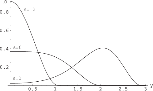
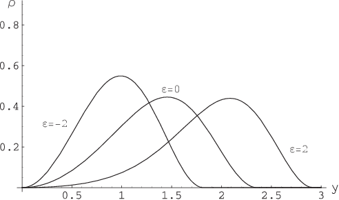
where $\Phi(a,c;x)$ is the confluent hypergeometric function (see, e.g., GrRy). As above we can take only the part of the solution (55) defined on the segment between two nearest to the minimum of the potential zeros of $\rho(x)$ and continue it on the residual part of the line by zero. It is permissible because $\rho(x)$ has degenerate zeroes. Then for an arbitrary value of the parameter $\varepsilon$ these distributions are bounded and have finite norms (see Fig. 1). Otherwise the integral of $\rho(x)$ diverges logarithmically.

It is not difficult to obtain the asymptotic at $x\rightarrow+\infty$ of a one-dimensional stationary solution to (33) for $A^{0}=V(x)$ , $\mathbf{A}=0$ :

\rho\sim\frac{\cos^{2}[\hbar^{-1}\int(2mV)^{1/2}dx]}{ZV^{1/2}},

(56)

where $V\rightarrow+\infty$ is assumed. The probability density function $\rho(x)$ has a finite norm if $V(x)$ increases more rapidly than $x^{2}$ at both infinities.

III.2 Relativistic particle

In this subsection we stochastically quantize the model of a relativistic particle interacting with the electromagnetic fields. As the result we obtain a relativistic generalization of the Fokker-Planck equation in the coordinate space. This model also serves as a simple example of a model with constraints.

The Hamiltonian action for an interacting relativistic particle has the form⁶⁶ 6 In this subsection $d$ is a dimension of the space-time and $x$ denotes a set of coordinates on it.

S_{H}[x,p,\lambda]=\int d\tau[p_{\mu}\dot{x}^{\mu}-\lambda((p-A)^{2}+m^{2})],

(57)

where $A_{\mu}$ is the electromagnetic potential. The dynamics of the model (57) is governed by the one constraint of the first kind.

According to the standard BFV-quantization scheme of the models with constraints of the first kind (see, e.g., HeTe) we introduce a canonically conjugated ghost pair $(c,P)$ and construct the BRST-charge

\Omega=c((p-A)^{2}+m^{2}),\qquad\{\Omega,\Omega\}=0.

(58)

The quantum BRST-charge is obtained from the classical one by means of the von Neumann corresponding rules (4). A graded version of the commutation relations (3) for positions and momenta is held. Therefore the quantum BRST-charge is nilpotent but not Hermitian.

Then the physical state is defined as

\hat{\Omega}|\psi\rangle=0,\qquad\langle O|\hat{\Omega}=0,\;\;\Rightarrow\;\;[\hat{\Omega},\hat{\rho}]=0.

(59)

This definition of a physical state respects also the BRST-cohomologies structure, i.e., the average over a physical state of a BRST-exact operator vanishes. Explicitly, in the coordinate representation we have

[(\hbar\partial_{\mu}+A_{\mu})(\hbar\partial^{\mu}+A^{\mu})+m^{2}]\psi(x)=0,\qquad[(\hbar\partial_{\mu}-A_{\mu})(\hbar\partial^{\mu}-A^{\mu})+m^{2}]O(x)=0.

(60)

When the electromagnetic fields vanish these equations are the Klein-Gordon equations for tachyons⁷⁷ 7 For the interrelation between relativistic random walking models and relativistic wave equations see, for instance, GJKSch; RanMug..

The action functional for the system of equations (60) is

S[O,\psi]=\int d^{d}xO(x)[(\hbar\partial_{\mu}+A_{\mu})(\hbar\partial^{\mu}+A^{\mu})+m^{2}]\psi(x).

(61)

As in the nonrelativistic case the action possesses a gauge invariance under the transformations (29). The conserved $4$ -current looks like

j^{\mu}=\frac{1}{2m}\left[O(\hat{p}^{\mu}-A^{\mu})\psi-\psi(\hat{p}^{\mu}+A^{\mu})O\right],

(62)

where $\hat{p}_{\mu}=-\hbar\partial_{\mu}$ . Making the substitution (32) into the system (60) we obtain a Lorentz-invariant generalization of the equations (33)

\partial^{\mu}\left[-\frac{\hbar}{2}\partial_{\mu}\rho+(\partial_{\mu}S-A_{\mu})\rho\right]=0,\qquad(\partial S-A)^{2}+m^{2}=-\hbar\partial^{\mu}(\partial_{\mu}S-A_{\mu}).

(63)

Again the first equation can be called as the relativistic Fokker-Planck equation in the coordinate space⁸⁸ 8 For the relativistic Fokker-Planck equation in the momentum space see, e.g., LandLif. For other approaches to a relativistic diffusion see, for example, DunHan; Fa; DTH., while the second equation is the quantum Hamilton-Jacobi equation. In the presence of the electromagnetic fields the integral

\int d\mathbf{x}\rho(t,\mathbf{x}),

(64)

is not an integral of motion. Analogously to quantum mechanics we can explain it by the pair creation.

In the absence of the electromagnetic fields there is a solution to the quantum Hamilton-Jacobi equation (63) in the form of a “plane wave”

S=p_{\mu}x^{\mu},\qquad p^{2}=-m^{2}.

(65)

Then the relativistic Fokker-Planck equation is rewritten as

p^{\mu}\partial_{\mu}\rho=\frac{\hbar}{2}\Box\rho.

(66)

That is the celebrated relativistic diffusion (heat) equation (see for the review JosPre). It is the hyperbolic type differential equation and, consequently, the propagation velocity of small fluctuations does not exceed the velocity of light contrary to the nonrelativistic diffusion equation. The integral (64) is conserved under an appropriate initial condition.

Notice that in the same fashion we can quantize the model of a nonrelativistic particle in the parameterized form

S_{H}[x,p,\lambda]=\int d\tau\left[p_{\mu}\dot{x}^{\mu}-\lambda(p_{0}+H(x,p))\right],

(67)

reproducing the results of the previous subsection.

IV Concluding remarks

There are at least two possible points of view on the results of this paper.

On the one hand we can consider the proposed quantization scheme from the position of deformation quantization. Then we investigate in this paper what happens when the algebra of observables is deformed by an imaginary parameter contrary to quantum mechanics with the real Planck constant. It would be intriguing if such a deformation results in a stochastic mechanics related in some way to real physics. The grounds for these hopes are provided by the observation that the obtained stochastic mechanics is closely related to the Langevin and Fokker-Planck equations and in the classical limit turns into classical mechanics.

On the other hand we can regard the proposed quantization procedure as another reformulation of the Langevin equation. This reformulation treats not only nonrelativistic and relativistic models in a uniform manner, but allows us to extend the developed methods of quantum mechanics to non-equilibrium statistic physics.

In both cases the work deserves further research. On this way we can distinguish the secondary stochastic quantization and its applications to the models with infinite degrees of freedom both in the relativistic and nonrelativistic cases. The most prominent models are of course the models of scalar and electromagnetic fields. Then we can attempt to attack the model of an incompressible fluid and compare the obtained stochastic model with the known one for the fully developed turbulence derived from the Langevin-Navier-Stokes equation (see for the review Ant).

Acknowledgements.

I am grateful to Prof. S.L. Lyakhovich for illuminating discussions on some aspects of deformation quantization. I appreciate I.V. Gorbunov and A.M. Pupasov for fruitful debates and the constructive criticism of the draft of this paper. This work was supported by the RFBR grant 06-02-17352 and the grant for Support of Russian Scientific Schools SS-5103.2006.2. The author appreciates financial support from the Dynasty Foundation and International Center for Fundamental Physics in Moscow.

References

(1) M. Namiki, Stochastic Quantization (Springer-Verlag, Berlin, 1992); M. Namiki, K. Okano eds., Stochastic quantization, Prog. Theor. Phys. Suppl. No. 111 (1993).
(2) G. Parisi, Statistical Field Theory (Addison-Wesley, Menlo Park, 1988).
(3) H. Risken, The Fokker-Planck Equation (Springer, Berlin, Heidelberg, 1989).
(4) J. Zinn-Justin, Quantum Field Theory and Critical Phenomena (Claredon Press, Oxford, 1996).
(5) E. Nelson, Derivation of the Shrödinger equation from Newtonian mechanics, Phys. Rev. 150, 1079 (1966); E. Nelson, Quantum Fluctuations (Princeton University Press, Princeton, New Jersey, 1985).
(6) F. Bayen, M. Flato, C. Fronsdal, A. Lichnerowicz, and D. Sternheimer, Deformation theory and quantization. I. Deformation of symplectic structures, Ann. Phys. 111, 61 (1978).
(7) D.D. Joseph, L. Preziosi, Heat waves, Rev. Mod. Phys. 61, 41 (1989); 62, 375 (1990).
(8) M. Henneaux, C. Teitelboim, Quantization of Gauge Systems (Princeton University Press, Princeton, New Jersey, 1992).
(9) S. Weinberg, The Quantum Theory of Fields. V.1. Foundations (Cambridge University Press, Cambridge, 2000).
(10) M. Chaichian, A. Demichev, Path Integrals in Physics. V.1. Stochastic Processes and Quantum Mechanics (Institute of Physics Publishing, Bristol, Philadelphia, 2001).
(11) B.V. Fedosov, A simple geometrical construction of deformation quantization, J. Differential Geom. 40, 213 (1994).
(12) M. Kontsevich, Defomation quantization of Poisson manifolds. I, Lett. Math. Phys. 66, 157 (2003). arXiv:q-alg/9709040.
(13) A.M. Scarfone, Stochastic quantization of an interacting classical particle system, J. Stat. Mech. 03012, (2007). arXiv:cond-mat/0703115.
(14) G. Litvinov, V. Maslov, and G. Shpiz, Idempotent (asymptotic) mathematics and the representation theory, arXiv:math/0206025.
(15) G.E. Uhlenbeck, L.S. Ornstein, On the theory of the Brownian motion, Phys. Rev. 36, 823 (1930).
(16) D. Leporini, R. Mauri, Fluctuations of non-conservative systems, J. Stat. Mech. 03002, (2007).
(17) I.S. Gradshteyn, I.M. Ryzhik, Table of Integrals, Series and Products. 5th edition (Academic Press, Boston, 1994).
(18) B. Gaveau, T. Jacobson, M. Kac, and L.S. Schulman, Relativistic extension of the analogy between quantum mechanics and Brownian motion, Phys. Rev. Lett. 53, 419 (1984).
(19) A. Ranfangni, D. Mugnai, Stochastic model for tunneling process: The question of superluminal behavior, Phys. Rev. E 52, 1128 (1995).
(20) E.M. Lifshits, L.P. Pitaevskii, Physical Kinetics, (Pergamon, Oxford, 1981).
(21) J. Dunkel, P. Hänggi, Theory of relativistic Brownian motion: The (1+3)-dimensional case, Phys. Rev. E 71, 016124 (2005). arXiv:cond-mat/0505532.
(22) K.S. Fa, Analysis of the relativistic Brownian motion in momentum space, Braz. J. Phys. 36, 777 (2006).
(23) J. Dunkel, P. Talkner, and P. Hänggi, Relativistic diffusion processes and random walk models, Phys. Rev. D 75, 043001 (2007). arXiv:cond-mat/0608023.
(24) N.V. Antonov, Renormalization group, operator product expansion and anomalous scaling in models of turbulent advection, J. Phys. A: Math. Gen. 39, 7825 (2006).