Distributed Algorithms for Spectrum Allocation, Power Control, Routing, and Congestion Control in Wireless Networks
Abstract
We develop distributed algorithms to allocate resources in multi-hop wireless networks with the aim of minimizing total cost. In order to observe the fundamental duplexing constraint that co-located transmitters and receivers cannot operate simultaneously on the same frequency band, we first devise a spectrum allocation scheme that divides the whole spectrum into multiple sub-bands and activates conflict-free links on each sub-band. We show that the minimum number of required sub-bands grows asymptotically at a logarithmic rate with the chromatic number of network connectivity graph. A simple distributed and asynchronous algorithm is developed to feasibly activate links on the available sub-bands. Given a feasible spectrum allocation, we then design node-based distributed algorithms for optimally controlling the transmission powers on active links for each sub-band, jointly with traffic routes and user input rates in response to channel states and traffic demands. We show that under specified conditions, the algorithms asymptotically converge to the optimal operating point.
I Introduction
While offering the potential for ubiquitous and untethered communications, wireless networks typically demand more sophisticated resource management than wireline networks. Optimal resource allocation in large-scale wireless networks involves joint optimization across multiple layers as well as distributed implementation across network nodes. In this paper, we develop distributed algorithms which jointly allocate frequency spectrum, transmission powers, traffic input rates, and traffic routes on a node-by-node basis in order to minimize total cost in an interference-limited multi-hop wireless network.
While joint optimization involving power control, congestion control, and routing has been studied previously [1, 2, 3], a common shortcoming of the previous work is the failure to account for the constraint that a node cannot transmit and receive simultaneously on the same frequency band. For while some types of multi-user interference can be ameliorated by using advanced coding techniques, interference between a transmitter and a co-located receiver is very difficult to suppress due to the transmitted power being many orders of magnitude higher than the received power at the same node.22 2 Theoretically a node is able to subtract the transmission signals generated by itself from the received signals so that the self-interference can be perfectly cancelled out. In real decoders, however, the received signals are practically irrecoverable in the face of the overwhelming transmitted signals. The resulting constraint that a transmitter cannot be simultaneously active with a co-located receiver [4] on the same frequency band is referred to as the duplexing constraint. In practical wireless networks, the duplexing constraint appears to be quite fundamental, and thus must be observed by resource management schemes.
In this paper, we develop distributed resource allocation algorithms for wireless networks in accordance with the duplexing constraint. To accomplish this, we first devise a new spectrum allocation scheme which divides the spectrum into a sufficient number of frequency bands and activates co-located transmitters and receivers on different bands. We show that the minimum number of sub-bands needed for resolving duplexing conflicts is asymptotically logarithmic in the chromatic number33 3 The chromatic number of a graph is the minimum number of colors with which the vertices of the graph can be colored such that adjacent vertices have different colors. of the network connectivity graph. We provide a simple algorithm that feasibly assigns frequency bands to links in a distributed and asynchronous manner with low control overhead.
Given a conflict-free spectrum allocation, we then design a set of node-based distributed gradient projection algorithms that iteratively adjust transmission powers, traffic input rates, and traffic routes according to channel conditions and traffic demands, in order to minimize total network cost. The power control and routing algorithms we develop are frequency selective, in that for each link, the power control algorithm adjusts the transmission power on each of the link’s active sub-bands. The routing algorithm involves both inter-node routing, which specifies the allocation of incoming traffic at each node to its outgoing links, and intra-node routing, which specifies the allocation of the total traffic on a given link across its active sub-bands. Finally, we show that congestion control can be naturally incorporated by considering an equivalent routing problem on a virtual overflow link. We show that under specified conditions, the iterative algorithms converge to the optimal operating point from any initial condition.
The rest of the paper is organized as follows. In Section II, we introduce the network model, discuss the duplexing constraint, and formulate the spectrum allocation problem. In Section III, we find the minimum number of sub-bands required by a feasible spectrum allocation. A distributed and asynchronous sub-band allocation algorithm is developed in Section IV. In Section V, we formulate the cross-layer optimization problem for networks operating on multiple sub-bands, and derive the conditions satisfied by the optimal configuration. In Section VI, we present node-based gradient projection algorithms to jointly optimize power control, routing, and congestion control based on the outcome of the spectrum allocation, as well as the channel conditions and traffic demands of the network.
II Network Model and Spectrum Allocation
Let the wireless network be modelled by a directed and connected graph , where is referred to as the connectivity graph of the network. A node represents a wireless transceiver, and represents a unidirectional wireless link from node to . We assume is link-symmetric, i.e., if , then , and vice versa. Two nodes and are neighbors if (or equivalently ). Let be the set of ’s neighbors.
II-A Duplexing Constrained Interference Model
We focus on a network model that prohibits any node from simultaneously transmitting and receiving on the same frequency band. That is, we impose the duplexing constraint on every band. Such a constraint is less stringent but more fundamental than the extensively studied primary interference constraint [5, 6, 7], where any node can transmit or receive (at any given time and on any given band) on at most one active link, and the secondary interference constraint, which further prohibits any node from transmitting when there is a neighbor receiving from another node [8]. A general approach to studying a broad class of interference constraints was presented in [9]. Indeed, duplexing constraints cannot be bypassed (at least currently) by using sophisticated coding methods, and must be observed by practical network management techniques.
Traditional network management techniques which aim to resolve various types of interference among wireless links have concentrated on scheduling in time [10, 11, 12, 13, 14, 15, 16, 17], where at any given time, only mutually-non-interfering links are activated. Scheduling, however, usually requires centralized controllers and involves high communication and computational complexity [7, 18]. Simplified distributed scheduling policies have been proposed [19, 8, 20, 5, 6] for various purposes. In general, however, the reduced implementation complexity comes at the expense of performance [21].
The difficulty in finding interference-free schedules in time leads us to seek an alternative solution. A natural approach is to consider network management in the domain of frequency instead of or in addition to time [22, 23, 24, 25]. Because communication on different frequency bands are practically non-interfering, one can think of simultaneously applying different link activation sets on non-overlapping frequency bands within the assigned spectrum. In this scheme, nodes transmit on certain bands while receiving on other bands to avoid duplexing interference. The spectrum allocation technique has an important advantage over scheduling in time: once a feasible spectrum allocation is established, the network can function relatively statically in that mode, not having to switch to another mode unless network itself changes substantially. While spectrum allocation problems have been proposed and studied in the interference graph induced by particular interference constraints, the solution using existing vertex-coloring methods [22, 23] is cumbersome and its complexity scales poorly with the size of the network. Moreover, the optimization of frequency assignment techniques has not been thoroughly investigated. In particular, the number of available frequency bands is often arbitrarily set and frequency bands are assigned to links in a heuristic manner [24, 25].
In this work, we adopt the spectrum allocation approach to resolve the fundamental duplexing conflicts for general wireless networks. In particular, we investigate two central questions: (1) what is the minimum number of frequency bands with which all co-located transmitters and receivers can be simultaneously activated subject to duplexing constraints, and (2) how can one efficiently find a feasible frequency assignment when there are enough frequency bands? We provide an exact analytical answer to question (1) and develop a distributed asynchronous algorithm which solves problem (2). Our analysis is based only the network connectivity graph. This approach requires much less storage and computation overhead than alternative methods that utilize the interference graph.
II-B Spectrum Division and Sub-band Allocation
The duplexing constraint permits only a subset of the links to be activated simultaneously on each frequency band. To activate all links at the same time, it is necessary to divide the spectrum into several sub-bands and activate different subsets of conflict-free links on different sub-bands.
Suppose the network occupies a contiguous spectrum which can be partitioned into a number, say , of sub-bands, each of which covers a contiguous segment of the whole spectrum. Let the collection of the sub-bands be denoted by . With a specific spectrum division in place, each link can be active on one or more of the sub-bands. If link uses sub-band , we say is an active link on , and is an active sub-band of . Denote the subset of links that are active on a sub-band by , and the set of active sub-bands of by . A spectrum allocation is given by the collection (or equivalently ). Note that finding a spectrum allocation involves two steps: spectrum division, which decides how many sub-bands the whole spectrum is divided into, and sub-band allocation, which determines which links are active on which sub-bands. We will address these two issues in Sections III and IV, respectively.
A spectrum allocation is feasible if (i) for all , , and (ii) for all , satisfies the duplexing constraint. Thus, any node’s outgoing and incoming links cannot be both active on the same sub-band. However, it is feasible for a node to have multiple active outgoing links or multiple active incoming links on a single sub-band.
II-C Interference Graph and Number of Sub-bands
In previous studies on frequency assignment techniques, the minimum number of frequency bands is found from the interference graph induced by the specific interference constraints [22, 23]. For the duplexing constraints, the interference graph is constructed as follows. Let the vertices of the interference graph be the links of the network connectivity graph , i.e., . In , an edge exists between two vertices (links in ) if one link’s transmitter is the other link’s receiver. The interference graph, unlike the connectivity graph, is undirected.44 4 In order to avoid confusion, we refer to the connectivity graph as having nodes and links , and the interference graph as having vertices and edges . It is easy to see that a feasible spectrum allocation on exists if and only if the number of available sub-bands is greater than or equal to the chromatic number of the interference graph . We illustrate the interference graph approach in Figure 1 using a complete four-node network. On the left is the connectivity graph , whose induced interference graph is shown in the middle. A minimal vertex-coloring on using four colors is depicted. The right graph represents the link-coloring on inferred by the minimal vertex-coloring on . The color(s) associated with each node are those assigned to the outgoing links of that node. The reason for using such a representation will be explained shortly.

Although the interference graph approach can provide an answer to our problem, it has major shortcomings. Note that the size of the interference graph is on the order of . To compute the chromatic number of , has to be constructed and stored at a central controller which then computes by finding a minimal vertex-coloring, which is itself an NP-complete problem [26]. For these reasons, the interference graph approach is not tractable for medium-and-large-scale networks. This motivates us to seek an alternative method that can find the minimum number of sub-bands directly from the connectivity graph .
III Spectrum Division
In this section, we investigate the minimum number of sub-bands which yields a feasible spectrum allocation. Our analysis will be based entirely on the network connectivity graph . For convenience of exposition, we first transform the problem into an equivalent graph-theoretic link-coloring problem.
III-A Link-Coloring Problem
For the moment, we leave the total number of sub-bands undetermined. Let each sub-band be identified by a unique color. We represent a spectrum allocation by a color assignment to links. A feasible spectrum allocation corresponds to a color assignment such that (i) all links are assigned with at least one color and (ii) for any node, no incoming link has a common color with any one of its outgoing links. We will find the minimum number of colors required for such a coloring. For any color assignment, denote the set of colors used by node ’s outgoing links by , and the set of colors used by its incoming links by . Since the network is connected and link-symmetric, every node has at least one outgoing and one incoming link, implying that and are both nonempty for all . A color assignment is feasible if and only if for all .55 5 Note that we allow one link to transmit on multiple sub-bands. Hence, we do not require or . Note that the feasibility of a coloring scheme can be checked using the node color sets , regardless of the detailed assignment of colors to links. In fact, we will show that studying the node outgoing color sets alone suffices for the link coloring problem. In the following, we say a color assignment is consistent with if results from the color assignment.
Lemma 1
Given a graph and the nodes’ outgoing color sets , there exists a consistent and feasible color assignment if and only if
(i) , for all ;
(ii) , for all .
Proof: We first prove the necessity part. Suppose first that (i) is violated, i.e., there exists a link such that , then must have a color in , meaning that some outgoing link of has the same color as , which is infeasible. Next suppose that (ii) does not hold for some node , i.e., there exists a color such that of every . Since is used on some outgoing link of , say , will have a color belonging to , violating the duplexing constraint at node .
The conditions are sufficient because given which satisfy (i)-(ii), a feasible coloring can be constructed by assigning each link the color(s) in . By (ii), this coloring is also consistent with . ∎
In the following, we use the shorthand notation to represent and . A collection of node outgoing color sets is said to be feasible if it satisfies the conditions in Lemma 1.
We now state the problem of finding the minimum number of sub-bands in terms of the minimal coloring problem as follows. Given a graph ,
| minimize | (1) | ||||
| subject to |
Denote the minimum number of colors by . To solve for , we first relax the constraints of problem (1) by dropping the second condition in Lemma 1 and consider
| minimize | (2) | ||||
| subject to |
where are any non-empty sets. The optimal solution to (2) must be less than or equal to . We will find a lower bound on and a matching upper bound on , thus uniquely determining . For lower bounding , the next observation is useful. The proof is deferred to Appendix -A.
Lemma 2
Let be distinct subsets of a -set all of which have the same cardinality . If , then there exist distinct subsets such that and , . If , then there exist distinct subsets such that and , .
Using Lemma 2 and the fact that any two distinct subsets , with the same cardinality satisfy , we can show the following (see the proof in Appendix -B).
Lemma 3
There exists an optimal solution for (2) such that all , , have the same cardinality.
Using Lemma 3, we can find a lower bound on as follows.
Lemma 4
Given a graph with chromatic number , the solution of the problem (2) is greater than or equal to , where the function is defined as
| (3) |
Proof: By Lemma 3, we can without loss of optimality consider a solution of (2) such that , for all . Therefore, whenever . Suppose there are distinct elements in . Because , by Sperner’s theorem [27], . Moreover, since satisfies the constraint in (2), we must have , where is the chromatic number of . Therefore, . ∎
Lemma 4 indicates that at least colors are needed to construct a feasible collection of node color sets even with the condition (ii) in Lemma 1 removed. However, by assigning node color sets according to a minimal node-labelling scheme of , colors are sufficient to yield a feasible configuration satisfying both conditions in Lemma 1. We can therefore conclude the following.
Lemma 5
Given a graph with chromatic number , the solution to the problem (1) is less than or equal to .
Proof: For graph , colors are sufficient because they can generate at least color subsets with equal cardinality , any two of which satisfy . Associate any of the color subsets with labels. Assign the color subsets to nodes according to a minimal node-labelling scheme, which requires exactly labels. We then have a feasible collection of node outgoing color sets that satisfies the two conditions in Lemma 1.66 6 An arbitrary color subset assignment according to a node-labelling solution generally results in satisfying only (i) in Lemma 1. Should (ii) not hold for some , reset . With this modification, both (i) and (ii) in Lemma 1 hold and no extra color is needed. ∎
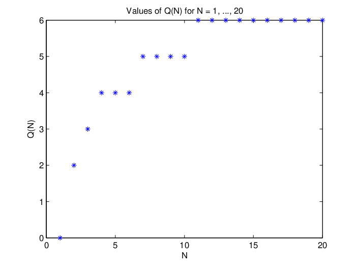
Proposition 1
It is easy to see that is nondecreasing. The values of for are plotted in Figure 2.
IV Distributed Sub-band Allocation
IV-A Spectrum Division Using Approximation of
We have found that the minimum number of sub-bands depends on the chromatic number . The problem of finding , however, is NP-complete [26] in general. On the other hand, any upper bound on gives us a sufficient number of sub-bands. One such well-known upper bound is , where is the maximum degree of any node in . In the following, we assume that there are at least sub-bands available.
The maximum degree is straightforward to determine (in a distributed manner), and we assume that it is known to all nodes a priori. Notice that is not too far from in typical networks,77 7 There are graphs, e.g. complete graphs, for which holds with equality. since the function is piecewise flat and grows approximately as a log function. It is worth comparing the upper bound with , an upper bound of , the chromatic number of the interference graph. Recall that vertices of are (directed) links of . Any vertex of has neighbors . Hence, by the assumption that is link-symmetric, the degree of in is given by
Here, and are the degrees of nodes and in . Consequently, the maximum degree of is
On the other hand, . Therefore, it is always true that
The equality holds only when the network topology is extremely asymmetric, e.g. the star networks. Typically, can be almost twice as large as . Moreover, the function is piecewise flat and scales as . The difference of the two upper bounds typically is substantial. Therefore, the connectivity graph approach developed in this work not only is more simple and straightforward but also leads to a tighter upper bound than the conventional interference graph approach.
IV-B Distributed Sub-band Allocation Algorithm
With the spectrum division accomplished, we now devise an algorithm with which feasible can be determined in a distributed manner and a feasible spectrum allocation can be found. The algorithm applies to all connected and link-symmetric graphs. Assume that sub-bands are available. For expositional purposes, we keep an unprocessed node set , which initially contains all the nodes. The Distributed Sub-band allocation (DSA) algorithm is iterated as follows.
Step 1. Initially . Arbitrarily select a node from and set . Arbitrarily choose sub-bands to form , mark as “processed”, and go to Step 2.
Step 2. Select an arbitrary node from such that has at least one processed neighbor (under the assumption that the network is connected, there is always such a node in after the first node is processed) and set . Node finds an with sub-bands which is different from all of its processed neighbors (it can be shown that such an always exists). Moreover, to maximally avoid potential channel interference, selects sub-bands in increasing order of their number of occurrences88 8 The number of occurrences can be zero. in (ties are broken arbitrarily).99 9 For instance, if the whole set of sub-bands is , and node finds its two neighbors have chosen and , it will accordingly choose either or . Mark as “processed”. If , repeat Step 2; otherwise go to Step 3.
Step 3. Each node allocates the sub-band(s) in to each outgoing link . The algorithm terminates.
Proposition 2
The set generated by the DSA algorithm induces a feasible spectrum allocation .
Proof: First we show that in Step 2 of the algorithm, an appropriate can always be found. Because the whole set has elements, there are at least distinct subsets with cardinality . However, has at most (processed) neighbors. Hence, there always exists at least one candidate for .
Now we show that the obtained up to Step 3 are feasible. They satisfy (i) in Lemma 1 due to the rule of successively selecting in Step 2. They also satisfy (ii) in Lemma 1, as proved next. Suppose on the contrary that there exists and such that for all . If is not the first processed node, the fact that implies that by the time is being determined, each of the sub-bands not included in must appear in every previously processed neighbor ’s . Taking also into account, we can deduce that all those have at least elements, which is a contradiction. Even if is the first processed node, the next processed node must be ’s neighbor and due to the algorithm’s rule. Hence, the hypothesis cannot be true in either case.
With the feasibility of the established, it is easy to verify that the generated in Step 3 induces a feasible spectrum allocation . ∎
In practice, the DSA algorithm can be implemented in a distributed fashion by nodes in the network. Specifically, after any node has arbitrarily set its at the beginning, any other node can determine its own as long as it has at least one processed neighbor and no other neighbor is being processed at the same instant. In other words, it is possible to have two non-adjacent nodes configuring their outgoing sub-bands at the same time. Since the action of a node depends only on its neighbors, node operations need not be globally coordinated or synchronized across the network. All that is required is an initialization phase that designates the first node to be processed. Thus, the sub-band allocation algorithm is distributed and asynchronous in nature.
Finally, we note that the DSA algorithm is robust to dynamic node failure and addition. Suppose that after a feasible spectrum allocation is established by the DSA algorithm, a node leaves the network. In this case, the configuration for the remaining nodes and links is still feasible. If a new node is to join the network, it can run Step 2 of the DSA algorithm to determine its own based on its neighbors’ . Then, active sub-bands for each link incident to can be allocated as in Step 3. As long as connects to at most nodes in the old network , the algorithm yields a feasible spectrum allocation for node , with all other nodes’ allocation unaffected.
V Cross-layer Optimization in Multi-radio Multi-hop Wireless Networks
The algorithm in Section IV generates a spectrum allocation where the active links on every sub-band satisfy the duplexing constraints. Given this feasible spectrum allocation, we now develop corresponding joint power control, routing, and congestion control algorithms which minimize total network cost, which will be specified later, given channel conditions and traffic demands.
V-A Interference Limited Transmissions and Node Power Constraints
We consider networks where messages on each sub-band are coded independently, and where the receiver of a link decodes its message on an active sub-band while treating all other signals on the same sub-band as interference. We assume that the capacity of link on a sub-band is a function of , the signal-to-interference-plus-noise ratio (SINR) of link over . Denoting the transmission powers used by the active links on sub-band by , we have
| (4) |
where is the path gain from to on sub-band , and is the power of the additive noise on sub-band at . Note that since the parameters and are sub-band-dependent, this framework is particularly appropriate for networks with frequency selective channels and colored noise.
Assume each node is limited by an individual power constraint , i.e.,
| (5) |
Denote the set of power variables that satisfy (5) by . In Section VI, we will design a set of power control algorithms that adjusts the power variables within the feasible region to minimize total network cost in conjunction with congestion control and routing.
V-B Traffic Demands, Congestion Control, and Routing
Let the traffic demands for the network consist of a collection of unicast sessions. Each (elastic) session is characterized by its fixed source-destination node pair and demand rate .1010 10 We assume that user gains no extra utility by transmitting at a rate higher than . So without loss of optimality, can be taken as the effective maximal incoming rate demanded by . We model the traffic as fluid flows. Assume congestion control is exercised at each source node. That is the source node can control the rate at which ’s traffic comes into the network. Denote the actual admitted rate of by , also referred to as the end-to-end flow rate of . Thus, the rate of the rejected traffic of , denoted by , is . After the admitted flow rates are determined by the congestion control at the source nodes, the flows entering the network are routed on (potentially) multiple paths from the source to destination. Let denote the rate of session traffic routed through link . The session flows satisfy the flow conservation constraints, i.e.,
| (6) |
| (7) |
and
| (8) |
Here, denotes both the total incoming and outgoing flow rates of session at an intermediate node . If we consider the rejected flow as being routed on a virtual “overflow” link from to [29, 30], the flow conservation constraint involving both real and virtual outgoing flows from the source node is given by
| (9) |
Thus, later on we will incorporate congestion control in a unified framework with routing. Let the set of flow vectors satisfying (7)-(9) be denoted by .
The total flow rate on link is . To route a flow of rate from to , node can split the traffic onto all active sub-bands of link and transmit them simultaneously. Let the rate of flow assigned to sub-band be . We have . Hence,
| (10) |
Note that the flow on each sub-band may consist of traffic of one or more sessions. However, the traffic split conserves the total rate of any session going through link . Therefore, at the receiver end of the link, node collects each session ’s traffic of rate .
One can think of the routing scheme as a two-step process. The first step determines inter-node routing, i.e., a feasible flow vector is found for every , yielding . The second step amounts to intra-node routing: each node routes the flow onto the active sub-bands available from to .
V-C Network Cost and Optimal Resource Allocation
The cost on each (real) link is made up of the costs incurred on its active sub-band(s) . Each is a function of , the SINR of link on , and , the flow rate on the active sub-band of link . Specifically, define
Assume that is decreasing and convex in for fixed , and that it is increasing and convex in for fixed . To impose the hard capacity constraint , where denotes the link capacity achieved by having , one can define for . An example of such cost functions is1111 11 For modelling purposes, we assume that on the transmitter side of each link there is one queue for every active sub-band of that link. Specifically, the arrival rate to the queue of link on sub-band is , the aggregate flow routed onto through . The cost function gives the expected delay in an M/M/1 queue with arrival rate and service capacity . In our present setting, is the sub-band specific link flow rate and is the sub-band specific link capacity. By the Kleinrock independence approximation and Jackson’s Theorem, the queue is a good approximation for the behavior of individual links on active sub-bands when the system involves Poisson stream arrivals at the entry points, a densely connected network, and moderate-to-heavy traffic load [31, 29]. where with constants .1212 12 The constants correspond to the bandwidth and processing gain of the system. The capacity formula is a good approximation for systems with a high processing gain, e.g. CDMA networks.
We associate an increasing and concave utility function , , to each (elastic) session . Thus, rejecting a flow of from the network incurs a utility loss of . This utility loss can also be interpreted as the cost on a virtual overflow link [29] with flow rate . Note that by definition, is increasing and convex in .
We solve for the feasible flow and power variables that jointly maximize the net utility, i.e., total utility minus total cost on real links. With the above observation, the maximization of net utility is equivalent to the problem of minimizing the total network cost consisting of costs on both real and overflow links. Formally, the Multi-Radio Minimum Cost Resource Allocation (MCRA) problem is
| minimize | ||||
| subject to | ||||
We will devise a distributed scheme that iteratively adjusts power control, routing and congestion control on a node-by-node basis so as to find the optimal solution to the MCRA problem.
V-D Control Variables and Optimality Conditions
To update transmission powers, traffic routes, and traffic input rates, we define the following power control and routing variables. These optimization variables are node-based and local in the sense that they are independently controlled at individual nodes.
V-D1 Power Control Variables
Let be the total power used by node on its active sub-band . Let be the power used by node on its outgoing link over an active sub-band . Define
constrained by
| (11) |
Also define
subject to constraints (let for )
| (12) |
With the above definitions, can be expressed in terms of the power control variables as
| (13) |
We use to denote the total interference and noise power of link on sub-band , i.e. the denominator of (13).
Define and . We now compute the partial derivative of the network cost with respect to each and . These partial derivatives are useful for characterizing the optimality conditions and for iterative adjustment of the power control variables. We have
| (14) |
where we have used shorthand notation for and defined
| (15) |
Note that as well as involves only local measures of . The partial derivative of with respect to is given by
| (16) |
where
| (17) |
is the message that node needs to send to any other node, say , which is active on in order for to compute via (16). Specifically, the message exchange works as follows.
Power Control Message Exchange Protocol: Let each node keep an up-to-date measure for each sub-band , where is derived by assembling the measures
on all its active incoming links on , and summing them up (cf. (17)). Note that is nonnegative and it is zero if has no active incoming link on . If , node broadcasts it to the whole network via a flooding protocol. This control message generating process is illustrated by Figure 3.

If , node collects and processes it according to the following rule. Node multiplies with the path gain .1313 13 In a symmetric duplex channel, , and node may use its own measurement of in the place of . Otherwise, it will need channel feedback from node to calculate . It further adds the product to the value of local measure if the origin of the message is a neighbor of and is active on sub-band . Finally, node adds up all the processed messages, and this sum multiplied by equals . Note that this protocol requires only one message from each node on each sub-band .1414 14 To be more precise, only the nodes having at least one active incoming link on a certain sub-band need to provide a message for that sub-band. Moreover in practice, node can ignore the messages generated by distant nodes, because they contribute very little to due to the negligible multiplicative factor on when and are far apart (cf. (16)).
V-D2 Routing Variables
Routing variables were first introduced by Gallager [32] for wireline network routing problems. Here, we define routing variables in a similar fashion. In addition to inter-node routing, however, routing variables here also perform the function of congestion control and intra-node routing.
Recall that congestion control is equivalent to routing a portion of traffic demand on a virtual overflow link directly from the source to the destination. Let be the source node of session , define overflow routing variable
which is constrained by . The overflow rate is then controlled by as , and the end-to-end flow rate is given by . Routing variables associated with a real link are defined by
which gives the fraction of the incoming flow of session at node that is routed onto link . At any node except the destination, of all satisfy
| (18) |
It is easy to see that the routing variables of all and uniquely determine the inter-node flow patterns of all sessions , and hence the total flow rate on links . Now let the flow allocation on active sub-bands be specified by the intra-node routing variables defined by
For any link , we must have
| (19) |
The link flow rate on an active sub-band is therefore given by
For notational brevity, denote by the vector if , or if . Also denote by the vector . We illustrate the use of the above routing variables by looking at a source node and one of its outgoing links in Figures 4 and 5. In Figure 4, the overflow link is marked by a solid line with hollow arrow.

In Figure 5, we assume that link is active on two sub-bands and , and that the inter-node flow rate from to is .

We now compute the partial derivative of with respect to those routing variables. First we have the derivative of with respect to the overflow routing variables
where is the marginal cost of increasing the end-to-end flow rate of session with all other variables held constant. This is a special case () of , which is the marginal cost of increasing the incoming flow rate of at node while keeping all other variables constant. These marginal costs are computed recursively as in [32]:
and for ,
| (20) | |||||
where we have used shorthand notation for and defined marginal routing cost indicators
| (21) |
Using , we can easily write out the partial derivative of in as
| (22) |
Finally, the partial derivative of in is given by
| (23) |
Notice that depends on local measures only. However, and are both tied to the value of of ’s downstream1515 15 Given a routing configuration of session , node is said to be downstream to if there exists a path , , , such that , , , are all positive. We say is upstream to with respect to session if is downstream to . neighbors , which in turn depends on of ’s downstream neighbors . Thus, we need a sequential message passing of the marginal routing costs, from the destination upstream to the source, to permit every node to acquire the partial derivatives in its local routing variables.
Routing Message Exchange Protocol: In [32], the rules for propagating the marginal routing cost information are specified. In order for node to evaluate the terms in (21), it needs to collect local measures from all as well as reports of marginal costs from its next-hop neighbors , for all traversing sessions . Moreover, it is responsible for calculating its own measure of marginal cost with respect to every session according to (20), and then providing the measure to its upstream neighbors with respect to the session . The sequential message passing terminates if and only if the routing pattern of the session contains no loops, which is guaranteed by the blocked-node-set technique developed in [32, 33].
V-D3 Conditions for Optimality
The power and routing configuration that solves the MCRA problem can be characterized in terms of the marginal power and routing costs as follows.
Theorem 1
For an instance of optimization variables to be optimal, the following conditions are necessary: For all and with ,
| (24) |
Moreover, for all ,
| (25) |
For all and , there exists a such that
| (26) |
and the constant satisfies
| (27) |
Furthermore, for such that , there exists a constant such that for all with ,
| (28) |
We sketch the proof of Theorem 1 in Appendix -C. First order conditions as in (24)-(28) are in general only necessary for a configuration to be optimal. However, they are further sufficient if the link cost function has certain convexity properties as we discuss next.
Let generically represent the SINR of a link on one of its active sub-bands. By (4), is a function of the power variables of all active links on the same sub-band, e.g. . Thus, is a function of the vector and . It turns out that a characterization of the sufficient conditions for optimality requires to be jointly convex in and . However, it can be shown that such a property is impossible given the assumption that is decreasing in .
One way to remedy this problem is to work with log-power variables, first introduced in [1, 2]. For each and , define . Consider as a function of and . If is jointly convex in and , the conditions in Theorem 1 are enough to imply the optimality of a configuration. The joint convexity property holds if and only if the link cost function satisfies the following.
Lemma 6
For all and , is jointly convex in and if and only if the matrix
| (29) |
is positive semidefinite for all .
In (29), and denote the first and second partial derivatives of with respect to , denotes the second partial derivative of with respect to , and denotes . It can be shown that the cost function with satisfies the condition in Lemma 6. Limited by the available space, we skip the proof of Lemma 6. We prove in Appendix -D that if the condition in Lemma 6 holds, the conditions stated in the next theorem are sufficient for optimality.
VI Node-Based Multi-Radio Power Control and Routing Algorithms
We develop a set of scaled gradient projection algorithms [34] by which individual nodes adjust their local power control and routing variables iteratively to achieve a global configuration satisfying the optimality conditions in Theorem 2. Each algorithm at a node updates the appropriate vector of local optimization variables, e.g. , , or , such that the updated vector results in a lower cost with all other variables held constant. This is achieved by updating the old vector in the opposite gradient direction scaled by an appropriate positive definite matrix, and projecting the new vector back into the feasible set whenever it falls outside. This technique has been applied to, for example, optimal routing in wireline networks [33] and optimal power control and routing in single-radio wireless networks [3].
VI-A Power Control Algorithms
We develop two sets of power control algorithms which let each node iteratively adjust the vector and the vector . First notice that if but contains only one of ’s outgoing links, say , must be equal to , and hence is not variable. Otherwise, if has more than one positive element, it is updated by the following scaled gradient projection algorithm:
| (30) |
Here, the superscripts , are the iteration indices, is a positive definite scaling matrix, is the vector , and is the projection operation onto the feasible set of (cf. (12)) relative to the norm induced by .1616 16 In general, , where is the feasible set of . To implement the algorithm (30), node needs the current value of , which by (15) is easily computable from local measures.
The algorithm used by node to iteratively update is as follows:
| (31) |
It has almost the same form as (30) except that the feasible set for the projection is defined by (11). However, notice that each component of depends on measures from all active links on sub-band . Therefore, prior to implementing (31), node needs to collect the appropriate power control messages to determine , as described by the message exchange protocol in Section V-D1.
VI-B Routing Algorithms
We now present the algorithm used by a node to update its inter-node routing vector for a traversing session . An iteration of the inter-node routing algorithm has the form
| (32) |
Here, is the vector of current marginal routing cost indicators and is a positive definite matrix used to scale the descent direction. The feasible set associated with the projection operation in (32) is prescribed by the constraint (18) and an additional requirement that for all , where is the blocked node set of node relative to session . The meaning and use of the blocked node set were briefly discussed in the routing message exchange protocol in Section V-D2. The exchange protocol also gives every node enough information to calculate the current prior to each iteration of (32).
For the source node of a session , the algorithm (32) is applied to the vector of routing variables associated with real outgoing links. The overflow routing variable is updated by
| (33) |
for which the projection is onto the feasible set . The gradient is given by subtracting , which is computable after the routing message exchange, from the local measure .
Finally, we come to the algorithm that node uses to iteratively adjust the intra-node routing vector applied to an outgoing link . The intra-node routing update is iterated as
| (34) |
Here, is the vector of partial derivatives of all , which are purely local measures. The scaling matrix is positive definite. The feasible set that the projection refers to is defined by (19).
VI-C Convergence of Algorithms
Having described the node-based power control and routing algorithms, we now state the main convergence result in the following theorem.
Theorem 3
Given a feasible spectrum allocation , let , , , be any feasible initial transmission power and routing configuration with finite cost. Then with appropriate scaling matrices, the update sequences , , and generated by the algorithms (30), (31), (32) and (34) converge, i.e., , , , and for all and as . Furthermore, the limiting configuration , , , satisfies the conditions in Theorem 2, and is a jointly optimal solution to the MCRA problem if the link cost function satisfies the condition in Lemma 6.
The proof hinges on the fact that, by using appropriate scaling matrices, every iteration of the algorithms (30), (31), (31) and (32) reduces the total cost of the MCRA problem until the optimality conditions in Theorem 2 are achieved. Finding the appropriate scaling matrices, however, is a major challenge. One approach to this problem is to choose the scaling matrices so that they upper bound the Hessian matrices with respect to the updated variables. In this way, the algorithms closely approximate Newton’s method, hence enjoying fast rate of convergence while simultaneously guaranteeing convergence from all initial conditions. This method has been successfully adopted in the power control and routing algorithms for single-radio wireless networks in [3], and can be generalized to the present context. Due to the limited space, however, we skip the details.
It is worth noting that convergence does not depend on any particular order of running the algorithms at different nodes. At any time, any node can update any set of its local optimization variables via the corresponding algorithm. All that is required for convergence is that each node iterates every algorithm until the adjusted variables have marginal costs satisfying conditions in Theorem 2. Finally, we note that convergence occurs from any initial configuration with finite cost. These features are crucial to the applicability of these algorithms to large networks which lack the ability of scheduling and synchronizing node operations.
Extensive simulations indicate that our algorithms are adaptive to time-varying network state, including channel fading, network topology, and traffic demand. Because every iteration of any algorithm always reduces the total cost under the current network condition, our scheme is able to constantly readjust routing and transmission powers towards the optimum that slowly shifts over time due to the network change.
VII Conclusion
We have developed an integrated cross-layer resource allocation scheme for general wireless multi-hop networks. To satisfy the fundamental duplexing constraints, our scheme first finds a feasible spectrum allocation by (1) dividing the whole spectrum into multiple sub-bands and (2) activating conflict-free links on each sub-band. Compared with traditional scheduling in time, the spectrum allocation technique has a number of advantages in operational simplicity and amenability to distributed and asynchronous implementation. By studying an equivalent combinatorial link-coloring problem, we found that the minimum number of sub-bands required by a feasible spectrum allocation is given by a simple function of the chromatic number of the network connectivity graph. The minimum number grows asymptotically at a logarithmic rate with the chromatic number, attesting to the good scalability of the spectrum allocation technique and its robustness to network topology changes. We designed a simple distributed and asynchronous algorithm by which a feasible spectrum allocation can be constructed given enough sub-bands.
Given a feasible spectrum allocation, we developed an analytical framework and a set of node-based distributed algorithms for optimally allocating transmission powers and traffic rates on active links. Such a framework is especially suitable for the design of wireless networks with frequency selective channels. We provided the conditions that an optimal power control and routing configuration must satisfy. We then designed a set of distributed power control and routing algorithms using the scaled gradient projection method. These algorithms can be iterated at individual nodes with little control overhead. Finally, we demonstrated that the algorithms asymptotically achieve the optimal configuration regardless of the initial condition and the order of iterating different algorithms.
-A Proof of Lemma 2
We provide the proof for the case . The other case can be seen as a corollary by taking complements of all subsets involved in the first case.
First notice that since , there are distinct subsets of cardinality , where , the number of distinct subsets of cardinality . Hence, the claim makes intuitive sense.
Consider the bipartite graph consisting of and where a pair of and are connected if and only if . In this case, is said to be a child of , and is said to be a parent of . It is easy to see that every has children and every has parents. Now the claim in the lemma is equivalent to the existence of a complete matching (of size ) of and in the bipartite graph specified above. Because implies that , the degree of any , which is , is greater than or equal to , the degree of any . In this case, a complete matching must exist by a corollary of Hall’s theorem (cf. Corollary 13.4 of [35]).
-B Proof of Lemma 3
Suppose is an optimal solution and . If does not have the property in the lemma, we can always modify it to which satisfies the property with being less than or equal to . Hence, the lemma follows. Suppose we have a feasible solution consisting of a collection of subsets . We show that based on , we can construct such that for all , where .
Define and . If , then or or both. If , define , replace each , , by subset with cardinality such that for all , and if and only if . Such a replacement is possible by Lemma 2. If , define , replace each , , by subset with cardinality such that for all , and if and only if . Such a replacement can be found also by Lemma 2. Denote by the subset of nodes whose is changed (either expanded or reduced). Because , is always non-empty. It can be verified that the new collection of subsets is another optimal solution of (2). If the minimum and maximum cardinalities of the new collection of subsets are equal, we are done. Otherwise repeat the above procedure until we obtain an even collection of subsets. The iterations terminate in a finite number of steps since each iteration strictly reduces the difference between and .
-C Proof of Theorem 1
We show that whenever one of conditions (24)-(28) is violated, the present configuration can be improved upon. We take condition (24) as an example. Arguments for the other conditions are similar. By (21) and (20), we have
and
Thus, condition (24) holds if and only if for all such that , for all . Suppose condition (24) is violated at with , i.e., there exists such that , for some . If and , there must exist with but for some other . Hence, the cost of the configuration can be further reduced by shifting a tiny portion from to as suggested by (23). If , then , we can reduce the cost by shifting a tiny portion from to in light of (22). If , then we can always make by setting all equal to zero but equal to one for one achieving the minimum in . Notice that reconfiguring does not change the value of since by assumption . Then, as before, the total cost can be further reduced by shifting a tiny portion from to .
-D Proof of Theorem 2
Suppose satisfies the conditions in Theorem 2. Suppose the configuration yields log-power variables and link flow variables , . Let be another feasible configuration which yields , , . Recall that each is jointly convex in and while each is convex in . Moreover, the feasible sets of log-power variables and flow variables are both convex. Therefore, the cost difference under the two configurations can be bounded by
| (35) | |||||
We will show that the RHS is nonnegative. We can re-write and lower bound the first two summations by the series of equalities and inequalities on the top of the next page.
For equality (a), we used the relation that
and appended terms which are all equal to zero by flow conservation constraints. Equality (b) is obtained by rewriting and as and , respectively, and reorganizing the terms. Condition (24) implies that
by which we obtain (c). The final inequality follows from condition (25).
Next we lower bound the third summation on the RHS of (35). To begin with, we switch the roles of and in the summation to rewrite it as
The partial derivative is computed as
Thus, we can expand the summation as shown in the second block on the next page.
| (36) | |||||
For the first summation on the RHS of (36), we use the convention that and for all . As a consequence, the summand vanishes if . Moreover, for those but , we can lower bound the summand by replacing with (cf. condition (28)) to get
It is implicit from (16) and (28) that . We thus can lower bound the first summation in (36) by
The inequality follows from the relation and that due to conditions (26) and (27).
Now consider the second summation on the RHS of (36). For each , let the summands with be lower bounded by
By condition (26), summands with are equal to
Therefore, the whole summation is lower bounded by
The second to last inequality is obtained by noting that due to condition (27) and the identity . The last inequality follows also from condition (27).
Thus, we have shown that the cost incurred by an arbitrary feasible configuration is greater than or equal to the cost by a configuration that satisfies the conditions in Theorem 2. So the proof is complete.
References
- [1] M. Johansson, L. Xiao, and S. Boyd, “Simultaneous routing and power allocation in CDMA wireless data networks,” in Proceedings of IEEE International Conference on Communications, vol. 1, May 2003.
- [2] M. Chiang, “To layer or not to layer: Balancing transport and physical layers in wireless multihop networks,” in Proceedings of IEEE INFOCOM 2004, vol. 4, Mar. 2004.
- [3] Y. Xi and E. M. Yeh, “Optimal distributed power control and routing in wireless networks,” in Proceedings of the 2006 International Symposium on Information Theory, (Seattle, WA), July 2006.
- [4] A. Goldsmith, Wireless Communications. Cambridge University Press, 2005.
- [5] L. Chen, S. H. Low, M. Chiang, and J. C. Doyle, “Jointly optimal congestion control, routing, and scheduling for wireless ad hoc networks,” in Proceedings of IEEE INFOCOM 2006, Apr. 2006.
- [6] L. Bui, A. Eryilmaz, R. Srikant, and X. Wu, “Joint asynchronous congestion control and distributed scheduling for multi-hop wireless networks,” in Proceedings of IEEE INFOCOM 2006, Apr. 2006.
- [7] B. Hajek and G. Sasaki, “Link scheduling in polynomial time,” IEEE Transactions on Information Theory, vol. 34, pp. 910–917, Sept. 1988.
- [8] E. Modiano, D. Shah, and G. Zussman, “Maximizing throughput in wireless networks via gossiping,” in Proceedings of ACM SIGMETRICS 2006, June 2006.
- [9] S. Ramanathan, “A unified framework and algorithm for (t/f/c)dma channel assignment in wireless networks,” in Proceedings of IEEE INFOCOM 1997, vol. 2, Apr. 1997.
- [10] L. Tassiulas and A. Ephremides, “Stability properties of constrained queueing systems and scheduling policies for maximum throughput in multihop radio networks,” IEEE Transactions on Automatic Control, vol. 37, no. 12, pp. 1936–1948, 1992.
- [11] N. McKeown, V. Anantharam, and J. Walrand, “Achieving 100% throughput in an input-queued switch,” in Proceedings of IEEE INFOCOM 1996, vol. 1, pp. 296–302, Mar. 1996.
- [12] D. N. Tse, “Multi-user diverstiy and proportional fairness.” US Patent 6449490.
- [13] V. Subramanian and R. Agrawal, “A stochastic approximation analysis of channel condition aware wireless scheduling algorithms,” in Proceedings of INFORMS Telecommunications Conference, 2002.
- [14] X. Liu, E. K. Chan, and N. B. Shroff, “Opportunistic transmission scheduling with resource-sharing constraints in wireless networks,” IEEE Journal on Selected Areas in Communications, Oct. 2001.
- [15] Y. Liu and E. Knightly, “Opportunistic fair scheduling over multiple wireless channels,” in Proceedings of IEEE INFOCOM 2003, Apr. 2003.
- [16] S. Borst, “User-level performance of channel-aware scheduling algorithms in wireless data networks,” in Proceedings of IEEE INFOCOM 2003, Apr. 2003.
- [17] T. ElBatt and A. Ephremides, “Joint scheduling and power control for wireless ad-hoc networks,” in Proceedings of IEEE INFOCOM 2002, pp. 976–984, June 2002.
- [18] E. Arikan, “Some complexity results about packet radio networks,” IEEE Transactions on Information Theory, vol. 31, pp. 910–918, 1984.
- [19] M. J. Neely, E. Modiano, and C. Rohrs, “Tradeoffs in delay guarantees and computation complexity for N N packet switches,” in Proceedings of the Conference on Information Sciences and Systems, (Princeton), Mar. 2002.
- [20] P. Chaporkar, K. Kar, and S. Sarkar, “Throughput guarantees through maximal scheduling in wireless networks,” in Proceedings of the 2005 Allerton Conference on Communication, Control and Computing, Sept. 2005.
- [21] X. Lin and N. Shroff, “The impact of imperfect scheduling on cross-layer rate control in wireless networks,” in Proceedings of IEEE INFOCOM 2005, vol. 3, pp. 1804–1814, Mar. 2005.
- [22] W. K. Hale, “Frequency assignment: theory and applications,” Proceedings of the IEEE, vol. 68, no. 12, pp. 1497–1514, 1980.
- [23] M. B. Cozzens and D.-I. Wang, “The general channel assignment problem,” Congressus Numerantium, vol. 41, pp. 115–129, 1984.
- [24] M. Alicherry, R. Bhatia, and L. Li, “Joint channel assignment and routing for throughput optimization in multi-radio wireless mesh networks,” in Proceedings of ACM Mobicom 2005, (Cologne, Germany), pp. 58–72, 2005.
- [25] M. Kodialam and T. Nandagopal, “Characterizing the capacity region in multi-radio multi-channel wireless mesh networks,” in Proceedings of the ACM Mobicom 2005, (Cologne, Germany), pp. 73–87, 2005.
- [26] M. R. Garey and D. S. Johnson, Computers and intractability: A guide to the theory of NP-completeness. W. H. Freeman and Company, 1979.
- [27] E. Sperner, “Ein satz über untermegen einer endlichen menge,” Math. Zeitschr, vol. 27, pp. 544–548, 1928.
- [28] W. Feller, An Introduction to Probability Theory and Its Applications. Wiley, 3rd ed., 1968.
- [29] D. Bertsekas and R. Gallager, Data Networks. Prentice Hall, second ed., 1992.
- [30] Y. Xi and E. M. Yeh, “Optimal capacity allocation, routing, and congestion control in wireless networks,” in Proceedings of the 2006 International Symposium on Information Theory, (Seattle, WA), July 2006.
- [31] L. Kleinrock, Communication Net: Stochastic Message Flow and Delay. New York: McGraw-Hill, 1964.
- [32] R. Gallager, “A minimum delay routing algorithm using distributed computation,” IEEE Transactions on Communications, vol. 25, no. 1, pp. 73–85, 1977.
- [33] D. Bertsekas, E. Gafni, and R. Gallager, “Second derivative algorithm for minimum delay distributed routing in networks,” IEEE Transactions on Communications, vol. 32, no. 8, pp. 911–919, 1984.
- [34] D. Bertsekas, Nonlinear Programming. Athena Scientific, second ed., 1999.
- [35] R. P. Grimaldi, Discrete and Combinatorial Mathematics. Addison Wesley, fifth ed., 2003.
| Yufang Xi (S’06) received the B. Sci degree in Electronic Engineering from Tsinghua University, Beijing, China, in 2003, and the M. Sci and M. Phil degrees in Electrical Engineering from Yale University, New Haven, CT, in 2005 and 2006, respectively. He is currently a Ph.D. candidate at the Department of Electrical Engineering at Yale. His research interests include cross-layer optimization and distributed resource allocation algorithms for wireless networks. |
| Edmund M. Yeh received his B.S. in Electrical Engineering with Distinction from Stanford University in 1994, M.Phil in Engineering from the University of Cambridge in 1995, and Ph.D. in Electrical Engineering and Computer Science from MIT in 2001. Since July 2001, he has been on the faculty at Yale University, New Haven, Connecticut, where he is currently an Associate Professor of Electrical Engineering and Computer Science. Dr. Yeh is a recipient of the Army Research Office (ARO) Young Investigator Program (YIP) Award (2003), the Winston Churchill Scholarship (1994), the National Science Foundation and Office of Naval Research Fellowships (1994) for graduate study, the Frederick E. Terman Award from Stanford University (1994) and the Barry M. Goldwater Scholarship from the United States Congress (1993). Dr. Yeh is a member of Phi Beta Kappa, Tau Beta Pi, and IEEE. He has been visiting faculty at MIT, Princeton University, University of California at Berkeley, and Swiss Federal Institute of Technology, Lausanne. |