跳到论文正文
W Papers独立论文阅读器 arXiv:0704.3616 论文正文 计算阅读时间 · 0%
引用这篇论文根据当前论文元数据生成,正式投稿前建议核对。


License: Assumed arXiv.org perpetual non-exclusive license
arXiv:0704.3616v2 [cond-mat.str-el] 01 Nov 2007

Entanglement and topological entropy of the toric code at finite temperature

Claudio Castelnovo1 and Claudio Chamon2 Affiliation: 1 Rudolf Peierls Centre for Theoretical Physics, University of Oxford, Oxford, OX1 3NP, UK
2 Physics Department, Boston University, Boston, MA 02215, USA
August 11, 2026
Abstract

We calculate exactly the von Neumann and topological entropies of the toric code as a function of system size and temperature. We do so for systems with infinite energy scale separation between magnetic and electric excitations, so that the magnetic closed loop structure is fully preserved while the electric loop structure is tampered with by thermally excited electric charges. We find that the entanglement entropy is a singular function of temperature and system size, and that the limit of zero temperature and the limit of infinite system size do not commute. The two orders of limit differ by a term that does not depend on the size of the boundary between the partitions of the system, but instead depends on the topology of the bipartition. From the entanglement entropy we obtain the topological entropy, which is shown to drop to half its zero-temperature value for any infinitesimal temperature in the thermodynamic limit, and remains constant as the temperature is further increased. Such discontinuous behavior is replaced by a smooth decreasing function in finite-size systems. If the separation of energy scales in the system is large but finite, we argue that our results hold at small enough temperature and finite system size, and a second drop in the topological entropy should occur as the temperature is raised so as to disrupt the magnetic loop structure by allowing the appearance of free magnetic charges. We discuss the scaling of these entropies as a function of system size, and how the quantum topological entropy is shaved off in this two-step process as a function of temperature and system size. We interpret our results as an indication that the underlying magnetic and electric closed loop structures contribute equally to the topological entropy (and therefore to the topological order) in the system. Since each loop structure per se is a classical object, we interpret the quantum topological order in our system as arising from the ability of the two structures to be superimposed and appear simultaneously.

I Introduction

Some strongly correlated quantum systems have rather rich spectral properties, such as ground state degeneracies that are not related to symmetries, but instead to topology. Haldane1985; Wen1990 Such systems are said to be topologically ordered, topo refs and they can have excitations with fractionalized quantum numbers, Arovas1984 as in the case of the fractional quantum Hall states. There have been proposals to utilize topologically ordered states for fault tolerant quantum computation, exploiting the resilience of these systems to decoherence by local perturbations or disturbances by the environment.

Levin and Wen Levin2006, and Kitaev and Preskill Kitaev2006 recently proposed that a characteristic signature of topological order can be found in a subleading correction of the Von Neumann (entanglement) entropy in systems prepared in (one of) its ground state(s). This topological correction to the entanglement entropy was indeed confirmed by exact calculations in discrete models exhibiting topological order, as well as in continuum systems such as fermionic Laughlin states. Haque2007 The notion of topological entropy provides a “non-local order parameter” for topologically ordered systems. Hereafter, we refer to topological order as characteristically identified by such non-vanishing topological entropy.

Although quantum topological order was introduced as a pure zero-temperature concept, is was recently shown Castelnovo2006 that a closely related behavior can be observed also in mixed state density matrices that describe classical systems in the presence of hard constraints. These findings show that topological order can survive thermal mixing under certain conditions, e.g., in hard constrained systems. Moreover, any possible experimental observation of quantum topological order must take into account the fact that the T=0T=0 limit is only an idealization and temperature, albeit small, is a perturbation that cannot be neglected. This is particularly relevant, for example, if one is interested in a practical application of topological order towards quantum computing, which will always be done at finite temperature. It is therefore interesting to study the behavior of topologically ordered systems as the temperature is gradually raised from zero, in search of a unified picture of topological order encompassing both the quantum zero-temperature limit and the classical hard-constrained limit.

In this paper, we investigate the fate of quantum topological order in the two-dimensional toric code on the square lattice in thermal equilibrium with a bath at finite temperature. In particular, we do so by studying the entanglement and topological entropies of the system, which we compute exactly.

We start from the zero-temperature limit of the model, which has been thoroughly studied in Ref. Kitaev2003. In this limit, the ground state (GS) of the system can be mapped onto two loop structures Hamma2006 each of which, we argue, is responsible for half of the topological contribution to the von Neumann entropy (i.e., half of the topological entropy of the system). As temperature is raised from zero, thermal equilibration disrupts (breaks) the loop structure and it is expected to destroy topological order. With an exact calculation in the limit where one of the two loop structures is fully preserved while the other is allowed to thermalize, Trebst2007 we show that the topological entropy gradually decreases as a function of temperature, for fixed and finite system size, from its zero-temperature value down to precisely half of that value. In particular, the temperature dependence of the topological entropy can be shown to appear always through the product KA​(T)​NK^{\ }_{A}(T)\,N, where KA​(T)K^{\ }_{A}(T) is a monotonic function of temperature with KA​(0)=0K^{\ }_{A}(0)=0 and KA​(∞)=∞K^{\ }_{A}(\infty)=\infty, and NN is an extensive quantity that scales linearly with the number of degrees of freedom in the system. Therefore, the thermodynamic limit N→∞N\to\infty and the T→0T\to 0 limit do not commute, and if the former is taken first, the topological entropy becomes a singular function at T=0T=0, and it equals one half of its zero-temperature value for any T≠0T\neq 0. In other words, in the thermodynamic limit any infinitesimal temperature is able to fully disrupt any loop structure for which we allow thermalization, and the contribution from this structure to the topological entropy is completely lost (irrespective of the presence of a finite energy gap). On the other hand, finite size systems can retain a statistical contribution to the topological entropy (in the sense that its value varies continuously with temperature) originating from a thermalized underlying loop structure.

From our results, we then infer the behavior of the finite-temperature topological entropy in the generic case, as illustrated in Fig. 1.

Refer to caption
Figure 1: Qualitative behavior of the topological entropy as a function of temperature TT and number of degrees of freedom 2​N2N, for the generic case where the two coupling constants in the model are well separated, i.e., λA≪λB\lambda^{\ }_{A}\ll\lambda^{\ }_{B}. The exact shape of the first crossover is shown in Fig. 5

For finite size systems, we expect to observe two continuous decays of the topological entropy, due to the gradual disruption of each of its two loop contributions. Each drop occurs when the number of corresponding defects ∼Ne−2λA,B/T\sim N\;e^{-2\lambda^{\ }_{A,B}/T}_{\ } reaches a value of order one, where 2​N2N is the number of degrees of freedom in the system, and λA\lambda^{\ }_{A} and λB\lambda^{\ }_{B} are the two coupling constants in the model, associated with one loop structure each. The separation between the two decays (the quantity Δ\Delta in the figure) is therefore proportional to the difference between the two coupling constants λA\lambda^{\ }_{A} and λB\lambda^{\ }_{B} in the Hamiltonian. Once again, if the thermodynamic limit is taken first, both decays collapse into a singular behavior where the topological entropy vanishes everywhere except for T=0T=0, where its value depends on the order between the thermodynamic and zero-temperature limit. Notice also that, although the crossover temperature Tcross(A,B)∼λA,B/ln⁡NT^{(A,B)}_{\rm cross}\sim\lambda^{\ }_{A,B}/\ln\sqrt{N} goes to zero in the limit of N→∞N\to\infty, it does so only in a logarithmic fashion.

The case of classical topological order is recovered in the present study when thermal fluctuations are allowed to completely break one of the loop structures while the other is strictly preserved. Indeed, this can be accomplished by imposing appropriate (local) hard constraints on the classical analog of the toric code. Castelnovo2006 Our results illustrate how both the concept of quantum topological order and of classical topological order are equally fragile, as they truly exist only in the zero-temperature / hard-constraint limit. Their effects however can extend well into the finite-temperature / soft-constraint realm – as our calculations show – so long as the size of the system is finite.

Our results suggest a simple pictorial interpretation of quantum topological order, at least for systems where there is an easy identification of loop structures as in the case here studied. The picture is that (i) the two loop structures contribute equally and independently to the topological order at zero temperature; (ii) each loop structure per se is a classical (non-local) object carrying a contribution of ln⁡D\ln D to the topological entropy (D=2D=2 being the so-called quantum dimension of the system); and (iii) the quantum nature of the zero-temperature system resides in the fact that two independent loop structures can be superimposed (therefore leading to an overall topological entropy equal to 2​ln⁡D=ln⁡D22\ln D=\ln D^{2}_{\ }). In this sense, our results lead to an interpretation of quantum topological order, at least for systems with simple loop structures, as the quantum mechanical version of a classical topological order (given by each individual loop structure).

We also investigate the von Neumann (entanglement) entropy SVNS^{\ }_{\textrm{VN}} as a function of temperature and system size. For instance, we show that, given any bipartition (𝒜,ℬ)(\mathcal{A},\mathcal{B}) of the whole system 𝒮=𝒜∪ℬ\mathcal{S}=\mathcal{A}\cup\mathcal{B}, the quantity

Δ​S\displaystyle\Delta S =\displaystyle= limT→0,L→∞SVN𝒜​(T)−limL→∞,T→0SVN𝒜​(T)\displaystyle\lim_{T\to 0,L\to\infty}S^{\mathcal{A}}_{\textrm{VN}}(T)-\lim_{L\to\infty,T\to 0}S^{\mathcal{A}}_{\textrm{VN}}(T) (1)
=\displaystyle= (mℬ−1)​ln⁡2,\displaystyle(m^{\ }_{\mathcal{B}}-1)\ln 2,

where SVN𝒜​(T)S^{\mathcal{A}}_{\textrm{VN}}(T) is the entropy of partition 𝒜\mathcal{A} after tracing out partition ℬ\mathcal{B}, mℬm^{\ }_{\mathcal{B}} is the number of disconnected regions in ℬ\mathcal{B}, and L=NL=\sqrt{N} is the linear size of the system. From this result, we learn that the topological contribution to the entanglement entropy can be filtered out directly from a single bipartition, provided mℬ>1m^{\ }_{\mathcal{B}}>1, as opposed to the constructions in Refs. Levin2006; Kitaev2006 that require a linear combination over multiple bipartitions.

We also show that, as soon as the temperature is different from zero, the von Neumann entropy is no longer symmetric upon exchange of subsystem 𝒜\mathcal{A} and subsystem ℬ\mathcal{B}, and it acquires a term that is extensive in the number of degrees of freedom that have not been traced out (see Eq. (45)). Symmetry and dependence only on the boundary degrees of freedom, at least in the thermodynamic limit, can be recovered if one considers instead the mutual information

I𝒜​ℬ​(T)\displaystyle I^{\ }_{\mathcal{A}\mathcal{B}}(T) =\displaystyle= 12​[SVN𝒜​(T)+SVNℬ​(T)−SVN𝒜∪ℬ​(T)],\displaystyle\frac{1}{2}\left[\vphantom{\sum}S^{\mathcal{A}}_{\textrm{VN}}(T)+S^{\mathcal{B}}_{\textrm{VN}}(T)-S^{\mathcal{A}\cup\mathcal{B}}_{\textrm{VN}}(T)\right]\;, (2)

as we explicitly show in this paper. Notice that I𝒜​ℬ​(0)≡SVN𝒜​(0)=SVNℬ​(0)I^{\ }_{\mathcal{A}\mathcal{B}}(0)\equiv S^{\mathcal{A}}_{\textrm{VN}}(0)=S^{\mathcal{B}}_{\textrm{VN}}(0). Once again, the mutual information exhibits a singular behavior at zero temperature since the thermodynamic limit and the zero-temperature limit do not commute. We find that the explicit topological contribution to I𝒜​ℬ​(T)I^{\ }_{\mathcal{A}\mathcal{B}}(T) in the thermodynamic limit is −12​(m𝒜+mℬ−1)​ln⁡2-\frac{1}{2}\left(m^{\ }_{\mathcal{A}}+m^{\ }_{\mathcal{B}}-1\right)\ln 2, where m𝒜m^{\ }_{\mathcal{A}} (mℬ)(m^{\ }_{\mathcal{B}}) is the number of disconnected components of partition 𝒜\mathcal{A} (ℬ)(\mathcal{B}).

Although we consider here a very specific model, we believe that our results are of relevance to a broader context, at least at a qualitative level. For example, it would be interesting to investigate the specific behavior of systems where the underlying structures responsible for the presence of topological order are no longer identical to each other. This is the case of the three-dimensional extension of the toric code, where a closed loop structure becomes dual to a closed membrane structure. Wen-comment

The paper is organized as follows. In Section II we present the model and discuss its characteristic features and properties. In Section III we compute the von Neumann entropy of the system as a function of temperature and system size, in the limit of one of the coupling constants going to infinity. We then obtain the exact expression for the topological entropy in Sec. IV, and we illustrate its behavior with numerical results. Finally, we discuss the implications of our results for the system with finite coupling constants and we infer the full temperature and system size dependence of the topological entropy in Sec. V. Conclusions are drawn in Sec. VI.

II The finite-temperature toric code

The zero-temperature limit of the model considered here was studied by Kitaev in Ref. Kitaev2003. It can be represented by 2​N2N spin-1/21/2 degrees of freedom on the bonds of an L×LL\times L square lattice, N=L2N=L^{2}_{\ }, with periodic boundary conditions (toric geometry). The system is endowed with a Hamiltonian that can be written in terms of star and plaquette operators as

H=−λB∑plaquettes​pBp−λA∑stars​sAs,H=-\lambda^{\ }_{B}\sum^{\ }_{\textrm{plaquettes}\>p}B^{\ }_{p}-\lambda^{\ }_{A}\sum^{\ }_{\textrm{stars}\>s}A^{\ }_{s}, (3)

where λA\lambda^{\ }_{A} and λB\lambda^{\ }_{B} are two positive coupling constants, Bp=∏i∈pσizB^{\ }_{p}=\prod^{\ }_{i\in p}\sigma^{\textrm{z}}_{i}, and As=∏j∈sσjxA^{\ }_{s}=\prod^{\ }_{j\in s}\sigma^{\textrm{x}}_{j}, with ii labeling all four edges of plaquette pp and jj labeling all four bonds meeting at vertex ss of the square lattice. Notice that the Hamiltonian, all the BpB^{\ }_{p} operators and all the AsA^{\ }_{s} commute with each other, and one can diagonalize them simultaneously. Given that there are N−1N-1 independent plaquette operators and N−1N-1 independent star operators (∏p=1NBp=11=∏s=1NAs\prod^{N}_{p=1}B^{\ }_{p}=\hbox{\small 1\kern-4.2pt\normalsize 1}=\prod^{N}_{s=1}A^{\ }_{s}), the eigenvectors with fixed BpB^{\ }_{p} and AsA^{\ }_{s} quantum numbers form a 222^{2}_{\ }-dimensional space. Furthermore, one can show that the GS 44-fold degeneracy has a topological nature that can be split only by the action of non-local (system spanning) operators. The ground state wavefunctions of this model are known exactly, Kitaev2003 and can be written in the σz\sigma^{\textrm{z}}_{\ } basis as

|Ψ0⟩=1|G|1/2​∑g∈Gg⁡|0⟩,|\Psi^{\ }_{0}\rangle=\frac{1}{|G|^{1/2}_{\ }}\sum^{\ }_{g\in G}g|0\rangle, (4)

where GG is the Abelian group generated by all star operators {As}s=1N\{A^{\ }_{s}\}^{N}_{s=1}, modulo the fact that ∏s=1NAs=11\prod^{N}_{s=1}A^{\ }_{s}=\hbox{\small 1\kern-4.2pt\normalsize 1}, |G|=2N−1|G|=2^{N-1}_{\ } is the dimension of GG, and |0⟩=|σ1z​…​σnz⟩|0\rangle=|\sigma^{\textrm{z}}_{1}\,\ldots\,\sigma^{\textrm{z}}_{n}\rangle is any given state that satisfies the condition Bp​|0⟩=|0⟩B^{\ }_{p}|0\rangle=|0\rangle, ∀p\forall\,p. There are four inequivalent choices for |0⟩|0\rangle, corresponding to the four different topological sectors of the model. The choice of sector is immaterial to the results presented hereafter, since they all have the same entanglement, Hamma2005 and we will set |0⟩=|++…+⟩|0\rangle=|++\ldots+\rangle for convenience throughout the rest of the paper.

Notice that the system is symmetric upon exchange of σx\sigma^{\textrm{x}}_{\ } with σz\sigma^{\textrm{z}}_{\ } components and of stars with plaquettes on the lattice. In the σx\sigma^{\textrm{x}}_{\ }-basis, each site must have 00, 22 or 44 spins with a negative σx\sigma^{\textrm{x}}_{\ } component on the adjacent bonds. If we were to remove all the bonds with a negative σx\sigma^{\textrm{x}}_{\ } component, we would obtain a configuration of closed loops on the square lattice, where loops are allowed to cross but do not overlap. Once a convention is established on how to interpret sites entirely surrounded by spins with positive σx\sigma^{\textrm{x}}_{\ } component (e.g., as two different loop parts touching at the corner, say the up-right and down-left loops), then one can establish a one-to-one correspondence between all basis states and all loop configurations on the square lattice where loops cannot overlap and can at most touch at a corner in an up-right, down-left fashion (see Fig. 2).

Refer to caption
Figure 2: Illustration of the spin-loop correspondence discussed in the text. All vertices with two positive and two negative σx\sigma^{\textrm{x}}_{\ } components on the adjacent links can be obtained via appropriate rotations of the ones shown in the figure.

The same is true for the σz\sigma^{\textrm{z}}_{\ }-basis, but the loops now live on the dual lattice given by the centers of the plaquettes of the original lattice. This description of the GS of the toric code in terms of loop degrees of freedom gives a qualitative picture of the origin of the non-local behavior of the system from which the presence of topological order stems. In particular, given that the two simultaneous loop descriptions can be mapped one onto the other upon exchanging σx\sigma^{\textrm{x}}_{\ } with σz\sigma^{\textrm{z}}_{\ } as well as the square lattice with its dual, it is tempting to speculate that they contribute equally to the topological order present in the system, and each loop structure is responsible for precisely half of the topological entropy. Our exact calculations show that this naive picture is indeed correct: if either of the loop structures is exactly preserved while the other is destroyed, e.g., via coupling to a thermal bath, the topological entropy of the system lowers to half of its original value.

Based on the σx\sigma^{\textrm{x}}_{\ } and σz\sigma^{\textrm{z}}_{\ } loop description, all possible perturbations to the system can be qualitatively divided into three different classes: (i) those that couple to a σz\sigma^{\textrm{z}}_{\ }-like term, and are able – if sufficiently strong – to disrupt the underlying σx\sigma^{\textrm{x}}_{\ } loop structure, but not the σz\sigma^{\textrm{z}}_{\ } one; (ii) those that couple to a σx\sigma^{\textrm{x}}_{\ }-like term, with precisely the opposite effect; and (iii) those that couple to a σy\sigma^{\textrm{y}}_{\ }-like term, and are able – again, if the coupling constant is large enough – to disrupt both loop structures, thus leading to a vanishing topological entropy. A generic coupling to a thermal bath is likely to encompass all of the above terms and in the thermodynamic limit the vanishing of the topological entropy is unavoidable. For finite size systems and at low enough temperature, however, the relative scale of the two coupling constants λB\lambda^{\ }_{B} and λA\lambda^{\ }_{A} plays a crucial role in determining how effective each of the above terms is with respect to the others. In this paper we consider the case when the two energy scales are well separated, namely λB≫λA\lambda^{\ }_{B}\gg\lambda^{\ }_{A}, and we discuss qualitatively the behavior of the system as the separation becomes weaker and vanishes. A large separation between the two energy scales is indeed expected if we notice that the toric code is a lattice realization of a ℤ2\mathbb{Z}^{\ }_{2} gauge theory, where the two coupling constants λA\lambda^{\ }_{A} and λB\lambda^{\ }_{B} relate directly to the chemical potential of the electric and magnetic monopoles. gauge_refs On the ground of a large separation between the two energy scales in the Hamiltonian, three distinct temperature regimes can be outlined:

  • (a)

    T≪λA/ln⁡NT\ll\lambda^{\ }_{A}/\ln\sqrt{N}, when all thermal excitations have a small Boltzmann weight and for finite size systems at finite time scales the topological entropy effectively retains its zero temperature value because of the scarcity of defects that can disrupt the loop structure;

  • (b)

    λA/ln⁡N<T≪λB/ln⁡N\lambda^{\ }_{A}/\ln\sqrt{N}<T\ll\lambda^{\ }_{B}/\ln\sqrt{N}, when thermal excitations of the σz\sigma^{\textrm{z}}_{\ } type can disrupt the σx\sigma^{\textrm{x}}_{\ } loops structure, while the σx\sigma^{\textrm{x}}_{\ }-like excitations are rather unlikely to occur and they can be effectively neglected; and

  • (c)

    λB/ln⁡N<T\lambda^{\ }_{B}/\ln\sqrt{N}<T, when the appearance of all the three types of thermal excitations leads to the complete disruption of the topological contribution to the entanglement entropy.

(Notice that the opposite case, where λA≫λB\lambda^{\ }_{A}\gg\lambda^{\ }_{B}, leads to equivalent results based on the symmetry of the model.) The temperature range considered in this paper corresponds to regimes (a) and (b), where the σz\sigma^{\textrm{z}}_{\ } loop structure is effectively preserved for sufficiently small system sizes and time scales. We will then discuss how our results can be used to infer the behavior of the topological entropy across the whole temperature range, illustrated in Fig. 1.

Basically, one can define a temperature dependent defect separation length scales ξA,B∼eλA,B/T\xi^{\ }_{A,B}\sim e^{\lambda^{\ }_{A,B}/T}, so that as long as the sample size is below these corresponding scales, the system is free from the associated type of defects. Similarly, one can define temperature-dependent time scales for defects to appear. The toric code is fragile in the sense that 𝒪⁡(1){\cal O}(1) defects destroy its topological order, so that for practical considerations not only the temperature must be small compared to a gap, but the system size and the time scales must not be too large as well.

We now consider the simplification where the finite system length N≪ξB\sqrt{N}\ll\xi_{B}, so we can neglect defects in the σz\sigma^{\textrm{z}}_{\ } loop structure. Forbidding any defects in the σz\sigma^{\textrm{z}}_{\ } loop structure is equivalent to neglecting all thermal processes that violate the constraint ∏i∈pσiz=+1\prod^{\ }_{i\in p}\sigma^{\textrm{z}}_{i}=+1, ∀p\forall\,p. Therefore, the Hilbert space in the regime of interest and within the chosen topological sector (recall that |0⟩=|++…+⟩|0\rangle=|++\ldots+\rangle) is given by {g​|0⟩|g∈G}\{g|0\rangle\;|\;g\in G\}. The equilibrium properties of the system are then captured by the finite-temperature density matrix

ρ⁡(T)\displaystyle\rho(T) =\displaystyle= 1Z​e−β​H^\displaystyle\frac{1}{Z}\>e^{-\beta\hat{H}} (5)
=\displaystyle= ∑g,g′∈G⟨0|g​e−β​H​g​g′​|0⟩​g|0⟩​⟨0|​g​g′∑g∈G⟨0|g​e−β​H​g|0⟩,\displaystyle\frac{\sum_{g,g^{\prime}_{\ }\in G}\langle 0|ge^{-\beta H}_{\ }gg^{\prime}_{\ }|0\rangle\;g|0\rangle\langle 0|gg^{\prime}_{\ }}{\sum_{g\in G}\langle 0|ge^{-\beta H}g|0\rangle},

where we used the group property to write a generic element g′′∈Gg^{\prime\prime}_{\ }\in G as g′′=g​g′g^{\prime\prime}_{\ }=gg^{\prime}_{\ }, ∃!g′∈G\exists!\,g^{\prime}_{\ }\in G given g∈Gg\in G. Recall that all group elements, as well as their composition, are defined as products of star operators modulo the identity ∏s=1NAs=11\prod^{N}_{s=1}A^{\ }_{s}=\hbox{\small 1\kern-4.2pt\normalsize 1}.

For the model under consideration, it is convenient to rewrite the Hamiltonian (3) as

H\displaystyle H =\displaystyle= −λB​P−λA​S\displaystyle-\lambda^{\ }_{B}P-\lambda^{\ }_{A}S
P\displaystyle P =\displaystyle= ∑plaquettes​pBp\displaystyle\sum^{\ }_{\textrm{plaquettes}\>p}B^{\ }_{p}
S\displaystyle S =\displaystyle= ∑stars​sAs.\displaystyle\sum^{\ }_{\textrm{stars}\>s}A^{\ }_{s}. (6)

Notice that P​g​|0⟩=N​g​|0⟩Pg|0\rangle=Ng|0\rangle, ∀g∈G\forall\,g\in G, and therefore

⟨0|g​e−β​H​g​g′|0⟩\displaystyle\langle 0|ge^{-\beta H}gg^{\prime}_{\ }|0\rangle =\displaystyle= eβ​λB​N​⟨0|g​eβ​λA​S​g​g′|0⟩\displaystyle e^{\beta\lambda^{\ }_{B}N}_{\ }\langle 0|ge^{\beta\lambda^{\ }_{A}S}_{\ }gg^{\prime}_{\ }|0\rangle (7)
=\displaystyle= eβ​λB​N​⟨0|eβ​λA​S​g′|0⟩\displaystyle e^{\beta\lambda^{\ }_{B}N}_{\ }\langle 0|e^{\beta\lambda^{\ }_{A}S}_{\ }g^{\prime}_{\ }|0\rangle

where we used the fact that any gg commutes with SS by construction.

Now, recall the definition of a group element g∈Gg\in G, which can be symbolically represented by the notation g≡∏s∈gAsg\equiv\prod^{\ }_{s\in g}A^{\ }_{s} (modulo the identity ∏s=1NAs=11\prod^{N}_{s=1}A^{\ }_{s}=\hbox{\small 1\kern-4.2pt\normalsize 1}, i.e., g=∏s∈gAs=∏s∉gAsg=\prod^{\ }_{s\in g}A^{\ }_{s}=\prod^{\ }_{s\notin g}A^{\ }_{s}). Given the expansion

eβ​λA​S=∏stars​s[cosh⁡β​λA+sinh⁡β​λA​As],e^{\beta\lambda^{\ }_{A}S}=\prod_{\textrm{stars}\,s}\left[\cosh\beta\lambda^{\ }_{A}+\sinh\beta\lambda^{\ }_{A}\>A^{\ }_{s}\right], (8)

which follows from the definition S=∑s=1NAsS=\sum^{N}_{s=1}A^{\ }_{s} and from the fact that As2≡11A^{2}_{s}\equiv\hbox{\small 1\kern-4.2pt\normalsize 1}, one obtains

⟨0|eβ​λA​S​g′|0⟩=\displaystyle\langle 0|e^{\beta\lambda^{\ }_{A}S}_{\ }g^{\prime}_{\ }|0\rangle=
=⟨0|∏s[cosh⁡β​λA+sinh⁡β​λA​As]​∏s′∈g′As′|0⟩\displaystyle\qquad=\langle 0|\prod_{s}\left[\cosh\beta\lambda^{\ }_{A}+\sinh\beta\lambda^{\ }_{A}\>A^{\ }_{s}\right]\prod_{s^{\prime}_{\ }\in g^{\prime}_{\ }}A^{\ }_{s^{\prime}_{\ }}|0\rangle
=(cosh⁡β​λA)N​(tanh⁡β​λA)n⁡(g′)\displaystyle\qquad=\left(\cosh\beta\lambda^{\ }_{A}\right)^{N}\;\left(\tanh\beta\lambda^{\ }_{A}\right)^{n(g^{\prime}_{\ })}
+(cosh⁡β​λA)N​(tanh⁡β​λA)N−n⁡(g′),\displaystyle\qquad\;\;\;\;+\left(\cosh\beta\lambda^{\ }_{A}\right)^{N}\;\left(\tanh\beta\lambda^{\ }_{A}\right)^{N-n(g^{\prime}_{\ })}, (9)

where NN is the total number of stars in the system, and n⁡(g′)n(g^{\prime}_{\ }) is the number of flipped stars in g′g^{\prime}_{\ }. Notice that the ambiguity in the definition of g=∏s∈gAs≡∏s∉gAsg=\prod^{\ }_{s\in g}A^{\ }_{s}\equiv\prod^{\ }_{s\notin g}A^{\ }_{s} – namely the fact that if g′g^{\prime}_{\ } is given by the product of a set of AsA^{\ }_{s}, it is also given by the product of all other AsA^{\ }_{s} but for those in the set – does not affect the equation above. In fact, this ambiguity amounts to the mapping n⁡(g′)↔N−n⁡(g′)n(g^{\prime}_{\ })\leftrightarrow N-n(g^{\prime}_{\ }). Similarly,

Z\displaystyle Z =\displaystyle= ∑g∈G⟨0|g​e−β​H​g|0⟩\displaystyle\sum^{\ }_{g\in G}\langle 0|ge^{-\beta H}g|0\rangle (10)
=\displaystyle= |G|​eβ​λB​N​⟨0|∏stars​s[cosh⁡β​λA+sinh⁡β​λA​As]|0⟩\displaystyle|G|\,e^{\beta\lambda^{\ }_{B}N}_{\ }\langle 0|\prod_{\textrm{stars}\,s}\left[\vphantom{\sum}\cosh\beta\lambda^{\ }_{A}+\sinh\beta\lambda^{\ }_{A}\>A^{\ }_{s}\right]|0\rangle
=\displaystyle= |G|​eβ​λB​N​(cosh⁡β​λA)N​[1+(tanh⁡β​λA)N].\displaystyle|G|\,e^{\beta\lambda^{\ }_{B}N}_{\ }(\cosh\beta\lambda^{\ }_{A})^{N}\left[\vphantom{\sum}1+(\tanh\beta\lambda^{\ }_{A})^{N}\right].

Substituting Eq. (9) and Eq. (10) into Eq. (5) after relabeling KA=−ln⁡[tanh⁡(β​λA)]K^{\ }_{A}=-\ln[\tanh(\beta\lambda^{\ }_{A})] gives

ρ⁡(T)=∑g,g′∈G1|G|​[e−KA​n​(g′)+e−KA​(N−n⁡(g′))][1+e−KA​N]​g​|0⟩​⟨0|​g​g′.\rho(T)=\sum_{g,g^{\prime}_{\ }\in G}\frac{1}{|G|}\frac{\left[e^{-K^{\ }_{A}n(g^{\prime}_{\ })}_{\ }+e^{-K^{\ }_{A}\left(N-n(g^{\prime}_{\ })\right)}_{\ }\right]}{\left[1+e^{-K^{\ }_{A}N}\right]}\;g|0\rangle\langle 0|gg^{\prime}_{\ }. (11)

In the limit of T→0T\to 0 (β→∞\beta\to\infty), KA→0+K^{\ }_{A}\to 0^{+}_{\ }, all g′g^{\prime}_{\ } are equally weighed, and one recovers the density matrix of the zero-temperature Kitaev model. In the limit T→∞T\to\infty (β→0\beta\to 0), KA→∞K^{\ }_{A}\to\infty, all g′g^{\prime}_{\ } are exponentially suppressed except for g′=11g^{\prime}_{\ }=\hbox{\small 1\kern-4.2pt\normalsize 1}, and one recovers the mixed-state density matrix of the topologically ordered classical system discussed in Ref. Castelnovo2006.

III The Von Neumann entropy

Let us consider a generic bipartition of the system 𝒮\mathcal{S} into subsystem 𝒜\mathcal{A} and subsystem ℬ\mathcal{B} (𝒮=𝒜∪ℬ\mathcal{S}=\mathcal{A}\cup\mathcal{B}). Let us also define Σ𝒜\Sigma^{\ }_{\mathcal{A}} (Σℬ\Sigma^{\ }_{\mathcal{B}}) to be the number of star operators AsA^{\ }_{s} that act solely on spins in 𝒜\mathcal{A} (ℬ\mathcal{B}), and Σ𝒜​ℬ\Sigma^{\ }_{\mathcal{A}\mathcal{B}} as the number of star operators acting simultaneously on both subsystems. Clearly these quantities satisfy the relationship Σ𝒜+Σℬ+Σ𝒜​ℬ=N\Sigma^{\ }_{\mathcal{A}}+\Sigma^{\ }_{\mathcal{B}}+\Sigma^{\ }_{\mathcal{A}\mathcal{B}}=N. Whenever a partition is made up of multiple connected components, e.g., 𝒜=𝒜1∪…∪𝒜m𝒜\mathcal{A}=\mathcal{A}^{\ }_{1}\cup\,\ldots\,\cup\mathcal{A}^{\ }_{m^{\ }_{\mathcal{A}}} with 𝒜i∩𝒜j=∅\mathcal{A}^{\ }_{i}\cap\mathcal{A}^{\ }_{j}=\emptyset and 𝒜i\mathcal{A}^{\ }_{i} connected, ∀i,j\forall\,i,j, let us denote with Σ𝒜i\Sigma^{\ }_{\mathcal{A}^{\ }_{i}} the number of star operators acting solely on 𝒜i\mathcal{A}^{\ }_{i} (Σ𝒜=∑iΣ𝒜i\Sigma^{\ }_{\mathcal{A}}=\sum^{\ }_{i}\Sigma^{\ }_{\mathcal{A}^{\ }_{i}}). [Since in the following we will consider only the case where either 𝒜\mathcal{A} or ℬ\mathcal{B} have multiple connected components, but not both at the same time, Σ𝒜​ℬi\Sigma^{\ }_{\mathcal{A}\mathcal{B}^{\ }_{i}} will be used unambiguously to denote the number of star operators acting simultaneously on 𝒜i\mathcal{A}^{\ }_{i} and on ℬ\mathcal{B} or on ℬi\mathcal{B}^{\ }_{i} and on 𝒜\mathcal{A}, according to the specific case (Σ𝒜​ℬ=∑iΣ𝒜​ℬi\Sigma^{\ }_{\mathcal{A}\mathcal{B}}=\sum^{\ }_{i}\Sigma^{\ }_{\mathcal{A}\mathcal{B}^{\ }_{i}}).]

The von Neumann (entanglement) entropy SVNS^{\ }_{\textrm{VN}} of a bipartition (𝒜,ℬ)(\mathcal{A},\mathcal{B}) is given by

SVNA≡−Tr​[ρA​ln⁡ρA]=SVNB,S^{A}_{\textrm{VN}}\equiv-\textrm{Tr}\left[\rho^{\ }_{A}\ln\rho^{\ }_{A}\right]=S^{B}_{\textrm{VN}}, (12)

where ρA=Trℬ​(ρ)\rho^{\ }_{A}=\textrm{Tr}^{\ }_{\mathcal{B}}(\rho) is the reduced density matrix obtained from the full density matrix ρ\rho by tracing out the degrees of freedom of subsystem BB, and the last equality holds whenever the full density matrix ρ\rho is a pure-state density matrix.

In order to compute the von Neumann entropy (12) from the finite-temperature density matrix (11), we first obtain the reduced density matrix of the system using the same approach of Ref. Hamma2005,

ρ𝒜​(T)\displaystyle\rho^{\ }_{\mathcal{A}}(T) =\displaystyle= ∑g,g′∈G1|G|[e−KA​n​(g′)+e−KA​(N−n⁡(g′))][1+e−KA​N]×\displaystyle\sum_{g,g^{\prime}_{\ }\in G}\frac{1}{|G|}\frac{\left[e^{-K^{\ }_{A}n(g^{\prime}_{\ })}_{\ }+e^{-K^{\ }_{A}\left(N-n(g^{\prime}_{\ })\right)}_{\ }\right]}{\left[1+e^{-K^{\ }_{A}N}\right]}\times (13)
g𝒜​|0𝒜⟩​⟨0𝒜|g𝒜​g𝒜′​⟨0ℬ|​gℬ​gB′​gℬ|0ℬ⟩\displaystyle\qquad\qquad g^{\ }_{\mathcal{A}}|0^{\ }_{\mathcal{A}}\rangle\langle 0^{\ }_{\mathcal{A}}|g^{\ }_{\mathcal{A}}g^{\prime}_{\mathcal{A}}\;\langle 0^{\ }_{\mathcal{B}}|g^{\ }_{\mathcal{B}}g^{\prime}_{B}g^{\ }_{\mathcal{B}}|0^{\ }_{\mathcal{B}}\rangle
=\displaystyle= ∑g∈G,g′∈G𝒜1|G|[e−KA​n​(g′)+e−KA​(N−n⁡(g′))][1+e−KA​N]×\displaystyle\sum_{g\in G,g^{\prime}_{\ }\in G^{\ }_{\mathcal{A}}}\frac{1}{|G|}\frac{\left[e^{-K^{\ }_{A}n(g^{\prime}_{\ })}_{\ }+e^{-K^{\ }_{A}\left(N-n(g^{\prime}_{\ })\right)}_{\ }\right]}{\left[1+e^{-K^{\ }_{A}N}\right]}\times
g𝒜​|0𝒜⟩​⟨0𝒜|​g𝒜​g𝒜′\displaystyle\qquad\qquad g^{\ }_{\mathcal{A}}|0^{\ }_{\mathcal{A}}\rangle\langle 0^{\ }_{\mathcal{A}}|g^{\ }_{\mathcal{A}}g^{\prime}_{\mathcal{A}}
≡\displaystyle\equiv 1|G|​∑g∈G,g′∈G𝒜ηT​(g′)​g𝒜​|0𝒜⟩​⟨0𝒜|​g𝒜​g𝒜′,\displaystyle\frac{1}{|G|}\sum^{\ }_{g\in G,g^{\prime}_{\ }\in G^{\ }_{\mathcal{A}}}\eta^{\ }_{T}(g^{\prime}_{\ })\;g^{\ }_{\mathcal{A}}|0^{\ }_{\mathcal{A}}\rangle\langle 0^{\ }_{\mathcal{A}}|g^{\ }_{\mathcal{A}}g^{\prime}_{\mathcal{A}},

where we used the generic tensor decomposition |0⟩=|0𝒜⟩⊗|0ℬ⟩|0\rangle=|0^{\ }_{\mathcal{A}}\rangle\otimes|0^{\ }_{\mathcal{B}}\rangle, g=g𝒜⊗gℬg=g^{\ }_{\mathcal{A}}\otimes g^{\ }_{\mathcal{B}}, and the fact that ⟨0ℬ|gℬ​gℬ′​gℬ|0ℬ⟩=1\langle 0^{\ }_{\mathcal{B}}|g^{\ }_{\mathcal{B}}g^{\prime}_{\mathcal{B}}g^{\ }_{\mathcal{B}}|0^{\ }_{\mathcal{B}}\rangle=1 if gℬ′=11ℬg^{\prime}_{\mathcal{B}}=\hbox{\small 1\kern-4.2pt\normalsize 1}^{\ }_{\mathcal{B}} and zero otherwise. The latter follows immediately from the fact that the group GG is Abelian and that As2=11A^{2}_{s}=\hbox{\small 1\kern-4.2pt\normalsize 1}, ∀s\forall\,s, and therefore gℬ2=11ℬg^{2}_{\mathcal{B}}=\hbox{\small 1\kern-4.2pt\normalsize 1}^{\ }_{\mathcal{B}} for any choice of ℬ\mathcal{B}. We also denoted by G𝒜={g∈G|gℬ=11ℬ}G^{\ }_{\mathcal{A}}=\{g\in G\;|\;g^{\ }_{\mathcal{B}}=\hbox{\small 1\kern-4.2pt\normalsize 1}^{\ }_{\mathcal{B}}\} the subgroup of GG given by all operations gg that act trivially on ℬ\mathcal{B} (similarly for GℬG^{\ }_{\mathcal{B}} in the following). For convenience of notation we defined

ηT​(g′)=[e−KA​n​(g′)+e−KA​(N−n⁡(g′))][1+e−KA​N].\eta^{\ }_{T}(g^{\prime}_{\ })=\frac{\left[e^{-K^{\ }_{A}n(g^{\prime}_{\ })}_{\ }+e^{-K^{\ }_{A}\left(N-n(g^{\prime}_{\ })\right)}_{\ }\right]}{\left[1+e^{-K^{\ }_{A}N}\right]}. (14)

Notice that a star operator AsA^{\ }_{s} can either act solely on spins in partition 𝒜\mathcal{A} (represented in the following by the notation s∈𝒜s\in\mathcal{A}), solely on spins in partition ℬ\mathcal{B} (s∈ℬs\in\mathcal{B}), or simultaneously on spins belonging to 𝒜\mathcal{A} and ℬ\mathcal{B} (which we will refer to as boundary star operators, and represent by s∈𝒜​ℬs\in\mathcal{A}\mathcal{B}). As discussed in Ref. Castelnovo2006, a complete set of generators for the subgroup G𝒜G^{\ }_{\mathcal{A}} can be constructed by taking: (i) all star operators that act solely on 𝒜\mathcal{A}, i.e., {As|s∈𝒜}\{A^{\ }_{s}\;|\;s\in\mathcal{A}\}, together with (ii) the collective operators defined as the product of all stars acting solely on a connected component of ℬ\mathcal{B} times the product of all boundary stars of that specific component, for all the mℬm^{\ }_{\mathcal{B}} connected components of ℬ\mathcal{B}, i.e., {∏s∈ℬiAs×∏s′∈𝒜​ℬiAs′,∀connected components​i}\{\prod^{\ }_{s\in\mathcal{B}^{\ }_{i}}A^{\ }_{s}\times\prod^{\ }_{s^{\prime}_{\ }\in\mathcal{A}\mathcal{B}^{\ }_{i}}A^{\ }_{s^{\prime}_{\ }},\;\forall\,\textrm{connected components}\,i\}. Notice that not all the collective operators are new operators with respect to those generated by the star operators in 𝒜\mathcal{A}. In fact, ∏i(∏s′∈ℬiAs′​∏s′′∈𝒜​ℬiAs′′)≡∏s∈𝒜As\prod^{\ }_{i}\left(\prod^{\ }_{s^{\prime}_{\ }\in\mathcal{B}^{\ }_{i}}A^{\ }_{s^{\prime}_{\ }}\prod^{\ }_{s^{\prime\prime}_{\ }\in\mathcal{A}\mathcal{B}^{\ }_{i}}A^{\ }_{s^{\prime\prime}_{\ }}\right)\equiv\prod^{\ }_{s\in\mathcal{A}}A^{\ }_{s}, and one can show that there are precisely mℬ−1m^{\ }_{\mathcal{B}}-1 new, independent operators. Consequently, the cardinality of the subgroup G𝒜G^{\ }_{\mathcal{A}} is given by d𝒜≡|G𝒜|=2ΣA+mℬ−1d^{\ }_{\mathcal{A}}\equiv|G^{\ }_{\mathcal{A}}|=2^{\Sigma^{\ }_{A}+m^{\ }_{\mathcal{B}}-1}_{\ }. Similarly for GℬG^{\ }_{\mathcal{B}}, dℬ≡|Gℬ|=2ΣB+m𝒜−1d^{\ }_{\mathcal{B}}\equiv|G^{\ }_{\mathcal{B}}|=2^{\Sigma^{\ }_{B}+m^{\ }_{\mathcal{A}}-1}_{\ }.

To proceed with the calculation of the von Neumann entropy of the finite temperature system, it is useful to use the above set of generators in order to represent the group G𝒜G^{\ }_{\mathcal{A}} in terms of Ising spin variables {θs,Θi}s∈𝒜connected components​i\{\theta^{\ }_{s},\,\Theta^{\ }_{i}\}^{\textrm{connected components}\,i}_{s\in\mathcal{A}}, where θs=−1\theta^{\ }_{s}=-1 (11) corresponds to the star operator AsA^{\ }_{s} appearing (not appearing) in the decomposition of g∈G𝒜g\in G^{\ }_{\mathcal{A}}, and similarly Θi=−1\Theta^{\ }_{i}=-1 (11) corresponds to the collective operator ∏s∈ℬiAs×∏s′∈𝒜​ℬiAs′\prod^{\ }_{s\in\mathcal{B}^{\ }_{i}}A^{\ }_{s}\times\prod^{\ }_{s^{\prime}_{\ }\in\mathcal{A}\mathcal{B}^{\ }_{i}}A^{\ }_{s^{\prime}_{\ }} appearing (not appearing) in the same decomposition. Notice that the correspondence is 22-to-11, since a configuration {θs,Θi}i,s\{\theta^{\ }_{s},\,\Theta^{\ }_{i}\}^{\ }_{i,s} and its spin-flipped counterpart {θ¯s,Θ¯i}i,s\{\overline{\theta}^{\ }_{s},\,\overline{\Theta}^{\ }_{i}\}^{\ }_{i,s}, where θ¯s=−θs\overline{\theta}^{\ }_{s}=-\theta^{\ }_{s} and Θ¯i=−Θi\overline{\Theta}^{\ }_{i}=-\Theta^{\ }_{i}, map onto the exact same g∈G𝒜g\in G^{\ }_{\mathcal{A}} (which follows from the fact that one of the collective operators can be generated out of the others appropriately combined with the star operators in 𝒜\mathcal{A}).

In this representation,

n⁡(g)\displaystyle n(g) =\displaystyle= ∑s1−θs​(g)2+∑i(Σℬi+Σ𝒜​ℬi)​1−Θi​(g)2\displaystyle\sum^{\ }_{s}\frac{1-\theta^{\ }_{s}(g)}{2}+\sum^{\ }_{i}\left(\Sigma^{\ }_{\mathcal{B}^{\ }_{i}}+\Sigma^{\ }_{\mathcal{A}\mathcal{B}^{\ }_{i}}\right)\frac{1-\Theta^{\ }_{i}(g)}{2} (15a)
=\displaystyle= N2−12​∑sθs​(g)−12​∑iΣ𝒫i​Θi​(g)\displaystyle\frac{N}{2}-\frac{1}{2}\sum^{\ }_{s}\theta^{\ }_{s}(g)-\frac{1}{2}\sum^{\ }_{i}\Sigma^{\ }_{\mathcal{P}^{\ }_{i}}\Theta^{\ }_{i}(g)
N−n⁡(g)\displaystyle N-n(g) =\displaystyle= ∑s1+θs​(g)2+∑i(Σℬi+Σ𝒜​ℬi)​1+Θi​(g)2\displaystyle\sum_{s}\frac{1+\theta^{\ }_{s}(g)}{2}+\sum^{\ }_{i}\left(\Sigma^{\ }_{\mathcal{B}^{\ }_{i}}+\Sigma^{\ }_{\mathcal{A}\mathcal{B}^{\ }_{i}}\right)\frac{1+\Theta^{\ }_{i}(g)}{2} (15b)
=\displaystyle= N2+12​∑sθs​(g)+12​∑iΣ𝒫i​Θi​(g),\displaystyle\frac{N}{2}+\frac{1}{2}\sum^{\ }_{s}\theta^{\ }_{s}(g)+\frac{1}{2}\sum^{\ }_{i}\Sigma^{\ }_{\mathcal{P}^{\ }_{i}}\Theta^{\ }_{i}(g),

where we used the fact that Σ𝒜+∑i(Σℬi+Σ𝒜​ℬi)=N\Sigma^{\ }_{\mathcal{A}}+\sum^{\ }_{i}\left(\Sigma^{\ }_{\mathcal{B}^{\ }_{i}}+\Sigma^{\ }_{\mathcal{A}\mathcal{B}^{\ }_{i}}\right)=N and we introduced the notation Σ𝒫i≡Σℬi+Σ𝒜​ℬi\Sigma^{\ }_{\mathcal{P}^{\ }_{i}}\equiv\Sigma^{\ }_{\mathcal{B}^{\ }_{i}}+\Sigma^{\ }_{\mathcal{A}\mathcal{B}^{\ }_{i}}.

Let us then use Eq. (13) to compute the nn-th power of ρ𝒜​(T)\rho^{\ }_{\mathcal{A}}(T):

ρ𝒜n​(T)\displaystyle\rho^{n}_{\mathcal{A}}(T) =\displaystyle= (1|G|)n∑g1∈Gg1′∈G𝒜…∑gn∈Ggn′∈G𝒜(∏l=1nηT(gl′))×\displaystyle\left(\frac{1}{|G|}\right)^{n}_{\ }\mathop{\sum_{g^{\ }_{1}\in G}}^{\ }_{g^{\prime}_{1}\in G^{\ }_{\mathcal{A}}}\ldots\mathop{\sum_{g^{\ }_{n}\in G}}^{\ }_{g^{\prime}_{n}\in G^{\ }_{\mathcal{A}}}\left(\prod^{n}_{l=1}\eta^{\ }_{T}(g^{\prime}_{l})\right)\times (16)
g1,𝒜​|0𝒜⟩​⟨0𝒜|g1,𝒜​g1,𝒜′​g2,𝒜|0𝒜⟩​⟨0𝒜|​g2,𝒜​g2,𝒜′\displaystyle g^{\ }_{1,\mathcal{A}}|0^{\ }_{\mathcal{A}}\rangle\langle 0^{\ }_{\mathcal{A}}|g^{\ }_{1,\mathcal{A}}g^{\prime}_{1,\mathcal{A}}g^{\ }_{2,\mathcal{A}}|0^{\ }_{\mathcal{A}}\rangle\langle 0^{\ }_{\mathcal{A}}|g^{\ }_{2,\mathcal{A}}g^{\prime}_{2,\mathcal{A}}
…​gn,𝒜​|0𝒜⟩​⟨0𝒜|​gn,𝒜​gn,𝒜′.\displaystyle\ldots g^{\ }_{n,\mathcal{A}}|0^{\ }_{\mathcal{A}}\rangle\langle 0^{\ }_{\mathcal{A}}|g^{\ }_{n,\mathcal{A}}g^{\prime}_{n,\mathcal{A}}.

Each expectation value above imposes gl,𝒜​gl,𝒜′​gl+1,𝒜=11𝒜g^{\ }_{l,\mathcal{A}}g^{\prime}_{l,\mathcal{A}}g^{\ }_{l+1,\mathcal{A}}=\hbox{\small 1\kern-4.2pt\normalsize 1}^{\ }_{\mathcal{A}}, l=1,…,n−1l=1,\ldots,n-1, and therefore gl​gl′​gl+1∈Gℬg^{\ }_{l}g^{\prime}_{l}g^{\ }_{l+1}\in G^{\ }_{\mathcal{B}}. Upon relabeling n−1n-1 summation variables so that g~l+1≡gl​gl′​gl+1\tilde{g}^{\ }_{l+1}\equiv g^{\ }_{l}g^{\prime}_{l}g^{\ }_{l+1} for l=1,…,n−1l=1,\ldots,n-1, the corresponding sums can then be combined with the respective inner product and they can be written as ∑g~l+1∈Gℬ1=dℬ\sum^{\ }_{\tilde{g}^{\ }_{l+1}\in G^{\ }_{\mathcal{B}}}1=d^{\ }_{\mathcal{B}}. Therefore, the equation above can be simplified to

ρ𝒜n​(T)\displaystyle\rho^{n}_{\mathcal{A}}(T) =\displaystyle= dℬn−1|G|n∑g1∈G(∏l=1n∑gl′∈G𝒜ηT(gl′))×\displaystyle\frac{d^{n-1}_{\mathcal{B}}}{|G|^{n}_{\ }}\sum_{g^{\ }_{1}\in G}\left(\prod^{n}_{l=1}\>\sum^{\ }_{g^{\prime}_{l}\in G^{\ }_{\mathcal{A}}}\eta^{\ }_{T}(g^{\prime}_{l})\right)\times (17)
g1,𝒜​|0𝒜⟩​⟨0𝒜|​g1,𝒜​g1,𝒜′​…​gn,𝒜′.\displaystyle g^{\ }_{1,\mathcal{A}}|0^{\ }_{\mathcal{A}}\rangle\langle 0^{\ }_{\mathcal{A}}|g^{\ }_{1,\mathcal{A}}g^{\prime}_{1,\mathcal{A}}\>\ldots\>g^{\prime}_{n,\mathcal{A}}.

Taking the trace of ρ𝒜n​(T)\rho^{n}_{\mathcal{A}}(T), using the fact that all the gg’s commute, and ∑g1∈G1=|G|\sum^{\ }_{g^{\ }_{1}\in G}1=|G|, one obtains

Tr​[ρ𝒜n]\displaystyle\textrm{Tr}\left[\rho^{n}_{\mathcal{A}}\right] =\displaystyle= (18)
=(dℬ|G|)n−1​∏l=1n∑gl′∈G𝒜ηT​(gl′)​⟨0𝒜|g1,𝒜′​…​gn,𝒜′|0𝒜⟩\displaystyle\!\!\!\!\!\!\!\!\!\!\!\!\!\!\!\!\!\!\!\!\!=\left(\frac{d^{\ }_{\mathcal{B}}}{|G|}\right)^{n-1}_{\ }\prod^{n}_{l=1}\>\sum^{\ }_{g^{\prime}_{l}\in G^{\ }_{\mathcal{A}}}\eta^{\ }_{T}(g^{\prime}_{l})\>\langle 0^{\ }_{\mathcal{A}}|g^{\prime}_{1,\mathcal{A}}\>\ldots\>g^{\prime}_{n,\mathcal{A}}|0^{\ }_{\mathcal{A}}\rangle
=(dℬ|G|)n−1​12n​∏l=1n∑{θs(l),Θi(l)}i,sconstr.ηT​({θs(l),Θi(l)}),\displaystyle\!\!\!\!\!\!\!\!\!\!\!\!\!\!\!\!\!\!\!\!\!=\left(\frac{d^{\ }_{\mathcal{B}}}{|G|}\right)^{n-1}_{\ }\frac{1}{2^{n}_{\ }}\prod^{n}_{l=1}\sum^{\textrm{constr.}}_{\{\theta^{(l)}_{s},\Theta^{(l)}_{i}\}^{\ }_{i,s}}\!\!\!\!\!\eta^{\ }_{T}(\{\theta^{(l)}_{s},\Theta^{(l)}_{i}\}),

where the factor of 1/2n1/2^{n}_{\ } comes from the 22-to-11 nature of the representation of G𝒜G^{\ }_{\mathcal{A}} in terms of Ising spin configurations, and the restricted summation ∑{θs(l),Θi(l)}constr.\sum^{\textrm{constr.}}_{\{\theta^{(l)}_{s},\Theta^{(l)}_{i}\}} is subject to the constraint ⟨0𝒜|g1,𝒜′​…​gn,𝒜′|0𝒜⟩≠0\langle 0^{\ }_{\mathcal{A}}|g^{\prime}_{1,\mathcal{A}}\>\ldots\>g^{\prime}_{n,\mathcal{A}}|0^{\ }_{\mathcal{A}}\rangle\neq 0, which can be explicitly stated in terms of the spins θs\theta^{\ }_{s} and Θi\Theta^{\ }_{i} as

{∏i,sδ(∏l=1nΘi(l)−1)δ(∏l=1nθs(l)−1)\displaystyle\left\{\prod^{\ }_{i,s}\delta(\prod^{n}_{l=1}\Theta^{(l)}_{i}-1)\delta(\prod^{n}_{l=1}\theta^{(l)}_{s}-1)\right.
+∏i,sδ(∏l=1nΘi(l)+1)δ(∏l=1nθs(l)+1)}.\displaystyle\qquad\qquad\qquad\left.+\prod^{\ }_{i,s}\delta(\prod^{n}_{l=1}\Theta^{(l)}_{i}+1)\delta(\prod^{n}_{l=1}\theta^{(l)}_{s}+1)\right\}.

Above and in the following, the short-hand notation i,si,s in sums and products stands for connected components​i\textrm{connected components}\,i and s∈𝒜s\in\mathcal{A}.

Let us then substitute Eqs. (15) into Eq. (14),

ηT​({θs(l),Θi(l)})\displaystyle\eta^{\ }_{T}(\{\theta^{(l)}_{s},\Theta^{(l)}_{i}\}) =\displaystyle= (19)
=cosh⁡(KA2​∑sθs(l)+KA2​∑iΣ𝒫i​Θi(l))cosh⁡(KA2​N)\displaystyle\!\!\!\!\!\!\!\!\!\!\!\!\!\!\!\!\!\!\!\!\!\!\!\!\!\!\!\!\!\!\!\!\!=\frac{\cosh\left(\frac{K^{\ }_{A}}{2}\sum^{\ }_{s}\theta^{(l)}_{s}+\frac{K^{\ }_{A}}{2}\sum^{\ }_{i}\Sigma^{\ }_{\mathcal{P}^{\ }_{i}}\Theta^{(l)}_{i}\right)}{\cosh\left(\frac{K^{\ }_{A}}{2}N\right)}
=12​cosh⁡(KA2​N)×\displaystyle\!\!\!\!\!\!\!\!\!\!\!\!\!\!\!\!\!\!\!\!\!\!\!\!\!\!\!\!\!\!\!\!\!=\frac{1}{2\cosh\left(\frac{K^{\ }_{A}}{2}N\right)}\times
∑J=±1eKA2​J​∑sθs(l)+KA2​J​∑iΣ𝒫i​Θi(l)\displaystyle\!\!\!\!\!\!\!\!\!\!\!\!\!\!\!\!\!\!\!\!\!\!\!\!\!\!\!\!\!\!\!\!\!\qquad\sum^{\ }_{J=\pm 1}e^{\frac{K^{\ }_{A}}{2}J\sum^{\ }_{s}\theta^{(l)}_{s}+\frac{K^{\ }_{A}}{2}J\sum^{\ }_{i}\Sigma^{\ }_{\mathcal{P}^{\ }_{i}}\Theta^{(l)}_{i}}_{\ }
=12​cosh⁡(KA2​N)×\displaystyle\!\!\!\!\!\!\!\!\!\!\!\!\!\!\!\!\!\!\!\!\!\!\!\!\!\!\!\!\!\!\!\!\!=\frac{1}{2\cosh\left(\frac{K^{\ }_{A}}{2}N\right)}\times
∑J=±1∏s∈𝒜eKA2​J​θs(l)​∏ieKA2​J​Σ𝒫i​Θi(l),\displaystyle\!\!\!\!\!\!\!\!\!\!\!\!\!\!\!\!\!\!\!\!\!\!\!\!\!\!\!\!\!\!\!\!\!\qquad\sum^{\ }_{J=\pm 1}\prod^{\ }_{s\in\mathcal{A}}e^{\frac{K^{\ }_{A}}{2}J\theta^{(l)}_{s}}_{\ }\prod^{\ }_{i}e^{\frac{K^{\ }_{A}}{2}J\Sigma^{\ }_{\mathcal{P}^{\ }_{i}}\Theta^{(l)}_{i}}_{\ },

and take the sum over all possible {θs(l),Θi(l)}i,s\{\theta^{(l)}_{s},\Theta^{(l)}_{i}\}^{\ }_{i,s} configurations (without any constraint),

[2​cosh⁡(KA2​N)]​∑{θs(l),Θi(l)}i,sηT​({θs(l),Θi(l)})=\displaystyle\left[2\cosh\left(\frac{K^{\ }_{A}}{2}N\right)\right]\sum^{\ }_{\{\theta^{(l)}_{s},\Theta^{(l)}_{i}\}^{\ }_{i,s}}\eta^{\ }_{T}(\{\theta^{(l)}_{s},\Theta^{(l)}_{i}\})=
=∑J=±1∑{θs(l),Θi(l)}i,s∏s∈𝒜eKA2​J​θs(l)​∏ieKA2​J​Σ𝒫i​Θi(l)\displaystyle\qquad=\sum^{\ }_{J=\pm 1}\sum^{\ }_{\{\theta^{(l)}_{s},\Theta^{(l)}_{i}\}^{\ }_{i,s}}\prod^{\ }_{s\in\mathcal{A}}e^{\frac{K^{\ }_{A}}{2}J\theta^{(l)}_{s}}_{\ }\prod^{\ }_{i}e^{\frac{K^{\ }_{A}}{2}J\Sigma^{\ }_{\mathcal{P}^{\ }_{i}}\Theta^{(l)}_{i}}_{\ }
=∑J=±1(∏s∑θs(l)=±1eKA2​J​θs(l))×\displaystyle\qquad=\sum^{\ }_{J=\pm 1}\left(\prod^{\ }_{s}\sum^{\ }_{\theta^{(l)}_{s}=\pm 1}e^{\frac{K^{\ }_{A}}{2}J\theta^{(l)}_{s}}_{\ }\right)\times
(∏i∑Θi(l)=±1eKA2​J​Σ𝒫i​Θi(l)).\displaystyle\qquad\qquad\qquad\left(\prod^{\ }_{i}\sum^{\ }_{\Theta^{(l)}_{i}=\pm 1}e^{\frac{K^{\ }_{A}}{2}J\Sigma^{\ }_{\mathcal{P}^{\ }_{i}}\Theta^{(l)}_{i}}_{\ }\right). (20)

Using the expression above, one can rewrite Eq. 18 as

Tr​[ρ𝒜n]\displaystyle\textrm{Tr}\left[\rho^{n}_{\mathcal{A}}\right] =\displaystyle= (dℬ|G|)n−1122​n​[cosh⁡(KA2​N)]n∏l=1n∑Jl=±1(∏s∑θs(l)=±1eKA2​Jl​θs(l))(∏i∑Θi(l)=±1eKA2​Jl​Σ𝒫i​Θi(l))×\displaystyle\left(\frac{d^{\ }_{\mathcal{B}}}{|G|}\right)^{n-1}_{\ }\frac{1}{2^{2n}_{\ }\left[\cosh\left(\frac{K^{\ }_{A}}{2}N\right)\right]^{n}_{\ }}\>\prod^{n}_{l=1}\sum^{\ }_{J^{\ }_{l}=\pm 1}\left(\prod^{\ }_{s}\sum^{\ }_{\theta^{(l)}_{s}=\pm 1}e^{\frac{K^{\ }_{A}}{2}J^{\ }_{l}\theta^{(l)}_{s}}_{\ }\right)\left(\prod^{\ }_{i}\sum^{\ }_{\Theta^{(l)}_{i}=\pm 1}e^{\frac{K^{\ }_{A}}{2}J^{\ }_{l}\Sigma^{\ }_{\mathcal{P}^{\ }_{i}}\Theta^{(l)}_{i}}_{\ }\right)\times
{∏i,sδ⁡(∏l=1nΘi(l)−1)​δ​(∏l=1nθs(l)−1)+∏i,sδ⁡(∏l=1nΘi(l)+1)​δ​(∏l=1nθs(l)+1)}\displaystyle\left\{\prod^{\ }_{i,s}\delta(\prod^{n}_{l=1}\Theta^{(l)}_{i}-1)\delta(\prod^{n}_{l=1}\theta^{(l)}_{s}-1)+\prod^{\ }_{i,s}\delta(\prod^{n}_{l=1}\Theta^{(l)}_{i}+1)\delta(\prod^{n}_{l=1}\theta^{(l)}_{s}+1)\right\}

and, upon expanding the product ∏l=1n(∑Jl=±1C⁡(Jl))=∑{Jl}l=1n∏l=1nC⁡(Jl)\prod^{n}_{l=1}\left(\sum^{\ }_{J^{\ }_{l}=\pm 1}C(J^{\ }_{l})\right)=\sum^{\ }_{\{J^{\ }_{l}\}^{n}_{l=1}}\prod^{n}_{l=1}C(J^{\ }_{l}), we obtain

Tr​[ρ𝒜n]\displaystyle\textrm{Tr}\left[\rho^{n}_{\mathcal{A}}\right] =\displaystyle= (dℬ|G|)n−1122​n​[cosh⁡(KA2​N)]n∑{Jl}l=1n{(∏s∑{θs(l)}l=1n∏θs(l)=+1eKA2​∑lJl​θs(l))(∏i∑{Θi(l)}l=1n∏Θi(l)=+1eKA2​∑lJl​Σ𝒫i​Θi(l))+\displaystyle\left(\frac{d^{\ }_{\mathcal{B}}}{|G|}\right)^{n-1}_{\ }\frac{1}{2^{2n}_{\ }\left[\cosh\left(\frac{K^{\ }_{A}}{2}N\right)\right]^{n}_{\ }}\>\sum^{\ }_{\{J^{\ }_{l}\}^{n}_{l=1}}\left\{\left(\prod^{\ }_{s}\mathop{\sum^{\ }_{\{\theta^{(l)}_{s}\}^{n}_{l=1}}}^{\ }_{\prod\theta^{(l)}_{s}=+1}e^{\frac{K^{\ }_{A}}{2}\sum^{\ }_{l}J^{\ }_{l}\theta^{(l)}_{s}}_{\ }\right)\left(\prod^{\ }_{i}\mathop{\sum^{\ }_{\{\Theta^{(l)}_{i}\}^{n}_{l=1}}}^{\ }_{\prod\Theta^{(l)}_{i}=+1}e^{\frac{K^{\ }_{A}}{2}\sum^{\ }_{l}J^{\ }_{l}\Sigma^{\ }_{\mathcal{P}^{\ }_{i}}\Theta^{(l)}_{i}}_{\ }\right)+\right. (21)
(∏s∑{θs(l)}l=1n∏θs(l)=−1eKA2​∑lJl​θs(l))(∏i∑{Θi(l)}l=1n∏Θi(l)=+1eKA2​∑lJl​Σ𝒫i​Θi(l))}\displaystyle\left.\left(\prod^{\ }_{s}\mathop{\sum^{\ }_{\{\theta^{(l)}_{s}\}^{n}_{l=1}}}^{\ }_{\prod\theta^{(l)}_{s}=-1}e^{\frac{K^{\ }_{A}}{2}\sum^{\ }_{l}J^{\ }_{l}\theta^{(l)}_{s}}_{\ }\right)\left(\prod^{\ }_{i}\mathop{\sum^{\ }_{\{\Theta^{(l)}_{i}\}^{n}_{l=1}}}^{\ }_{\prod\Theta^{(l)}_{i}=+1}e^{\frac{K^{\ }_{A}}{2}\sum^{\ }_{l}J^{\ }_{l}\Sigma^{\ }_{\mathcal{P}^{\ }_{i}}\Theta^{(l)}_{i}}_{\ }\right)\right\}

Notice that the indices ss and ii to the variables θs(l)\theta^{(l)}_{s} and Θi(l)\Theta^{(l)}_{i}, respectively, are mute since the sums over the possible values of θs(l)\theta^{(l)}_{s} and Θi(l)\Theta^{(l)}_{i} are performed first. Therefore one can simplify the notation above by replacing θs(l)→θ(l)\theta^{(l)}_{s}\to\theta^{(l)}_{\ } and Θi(l)→Θ(l)\Theta^{(l)}_{i}\to\Theta^{(l)}_{\ } for all ss and ii. Moreover, one can recognize that an Ising spin chain {θ(l)}\{\theta^{(l)}_{\ }\} with ∏θ(l)=±1\prod\theta^{(l)}_{\ }=\pm 1 is dual to an Ising spin chain {τl}\{\tau^{\ }_{l}\} with periodic / antiperiodic boundary conditions (using the 22-to-11 mapping θ(l)=τl​τl+1\theta^{(l)}_{\ }=\tau^{\ }_{l}\tau^{\ }_{l+1}). Thus,

∑{θ(l)}l=1n∏θ(l)=±1eKA2​∑l=1nJl​θ(l)\displaystyle\mathop{\sum^{\ }_{\{\theta^{(l)}_{\ }\}^{n}_{l=1}}}^{\ }_{\prod\theta^{(l)}_{\ }=\pm 1}e^{\frac{K^{\ }_{A}}{2}\sum^{n}_{l=1}J^{\ }_{l}\theta^{(l)}_{\ }}_{\ } =\displaystyle= 12​∑{τl}l=1np./a.eKA2​∑l=1nJl​τl​τl+1\displaystyle\frac{1}{2}\sum^{\textrm{p.}/\textrm{a.}}_{\{\tau^{\ }_{l}\}^{n}_{l=1}}e^{\frac{K^{\ }_{A}}{2}\sum^{n}_{l=1}J^{\ }_{l}\tau^{\ }_{l}\tau^{\ }_{l+1}}_{\ } (22)
≡\displaystyle\equiv 12​Zn(p/a)​(KA,{Jl}),\displaystyle\frac{1}{2}Z^{(p/a)}_{n}(K^{\ }_{A},\{J^{\ }_{l}\}),

where Zn(p/a)​(KA,{Jl})Z^{(p/a)}_{n}(K^{\ }_{A},\{J^{\ }_{l}\}) is the partition function of a chain of nn Ising spins with periodic / antiperiodic boundary conditions, in presence of a nearest-neighbor interaction with position-dependent reduced coupling constant KA​Jl/2K^{\ }_{A}J^{\ }_{l}/2. Similarly,

∑{Θ(l)}l=1n∏Θ(l)=±1eKA2​∑l=1nΣ𝒫i​Jl​Θ(l)\displaystyle\mathop{\sum^{\ }_{\{\Theta^{(l)}_{\ }\}^{n}_{l=1}}}^{\ }_{\prod\Theta^{(l)}_{\ }=\pm 1}e^{\frac{K^{\ }_{A}}{2}\sum^{n}_{l=1}\Sigma^{\ }_{\mathcal{P}^{\ }_{i}}J^{\ }_{l}\Theta^{(l)}_{\ }}_{\ } ≡\displaystyle\equiv 12​Zn(p/a)​(KA​Σ𝒫i,{Jl}),\displaystyle\frac{1}{2}Z^{(p/a)}_{n}(K^{\ }_{A}\Sigma^{\ }_{\mathcal{P}^{\ }_{i}},\{J^{\ }_{l}\}),

and Eq. (21) can be rewritten as

Tr​[ρ𝒜n]\displaystyle\textrm{Tr}\left[\rho^{n}_{\mathcal{A}}\right] =\displaystyle= 12Σ𝒜+mℬ(dℬ|G|)n−1122​n​[cosh⁡(KA2​N)]n∑{Jl}l=1n×\displaystyle\frac{1}{2^{\Sigma^{\ }_{\mathcal{A}}+m^{\ }_{\mathcal{B}}}_{\ }}\left(\frac{d^{\ }_{\mathcal{B}}}{|G|}\right)^{n-1}_{\ }\frac{1}{2^{2n}_{\ }\left[\cosh\left(\frac{K^{\ }_{A}}{2}N\right)\right]^{n}_{\ }}\>\sum^{\ }_{\{J^{\ }_{l}\}^{n}_{l=1}}\times
{(Zn(p)​(KA,{Jl}))Σ𝒜​∏i(Zn(p)​(KA​Σ𝒫i,{Jl}))+(Zn(a)​(KA,{Jl}))Σ𝒜​∏i(Zn(a)​(KA​Σ𝒫i,{Jl}))}.\displaystyle\left\{\left(Z^{(p)}_{n}(K^{\ }_{A},\{J^{\ }_{l}\})\right)^{\Sigma^{\ }_{\mathcal{A}}}_{\ }\prod^{\ }_{i}\left(\vphantom{\prod^{1}_{0}}Z^{(p)}_{n}(K^{\ }_{A}\Sigma^{\ }_{\mathcal{P}^{\ }_{i}},\{J^{\ }_{l}\})\right)+\left(Z^{(a)}_{n}(K^{\ }_{A},\{J^{\ }_{l}\})\right)^{\Sigma^{\ }_{\mathcal{A}}}_{\ }\prod^{\ }_{i}\left(\vphantom{\prod^{1}_{0}}Z^{(a)}_{n}(K^{\ }_{A}\Sigma^{\ }_{\mathcal{P}^{\ }_{i}},\{J^{\ }_{l}\})\right)\right\}.

The partition functions can be evaluated, for either boundary conditions, using a transfer matrix approach. For periodic boundary conditions, we obtain

Zn(p)​(K,{Jl})=Tr​[∏l=1nTl],Tl=(eK2​Jle−K2​Jle−K2​JleK2​Jl).Z^{(p)}_{n}(K,\{J^{\ }_{l}\})=\textrm{Tr}\left[\prod^{n}_{l=1}T^{\ }_{l}\right],\;\;\;\;\;\;T^{\ }_{l}=\left(\begin{array}[]{cc}e^{\frac{K}{2}J^{\ }_{l}}_{\ }&e^{-\frac{K}{2}J^{\ }_{l}}_{\ }\\ e^{-\frac{K}{2}J^{\ }_{l}}_{\ }&e^{\frac{K}{2}J^{\ }_{l}}_{\ }\end{array}\right).

Since all matrices TlT^{\ }_{l} are diagonalized by the same unitary matrix

U=12​(11−11),U=\frac{1}{\sqrt{2}}\left(\begin{array}[]{cc}1&1\\ -1&1\end{array}\right), (25)

and using the cyclic properties of the trace, we get

Zn(p)​(K,{Jl})\displaystyle Z^{(p)}_{n}(K,\{J^{\ }_{l}\}) =\displaystyle= Tr​[∏l=1n(U​Tl​U†)]\displaystyle\textrm{Tr}\left[\prod^{n}_{l=1}(UT^{\ }_{l}U^{\dagger}_{\ })\right]
=Tr​[∏l=1n(eK2​Jl+e−K2​Jl00eK2​Jl−e−K2​Jl)]\displaystyle\!\!\!\!\!\!\!\!\!\!\!\!\!\!\!\!\!\!\!\!\!\!\!\!\!\!\!=\textrm{Tr}\left[\prod^{n}_{l=1}\left(\begin{array}[]{cc}e^{\frac{K}{2}J^{\ }_{l}}_{\ }+e^{-\frac{K}{2}J^{\ }_{l}}_{\ }&0\\ 0&e^{\frac{K}{2}J^{\ }_{l}}_{\ }-e^{-\frac{K}{2}J^{\ }_{l}}_{\ }\end{array}\right)\right]
=Tr​[∏l=1n(2​cosh⁡(K2)002​Jl​sinh⁡(K2))]\displaystyle\!\!\!\!\!\!\!\!\!\!\!\!\!\!\!\!\!\!\!\!\!\!\!\!\!\!\!=\textrm{Tr}\left[\prod^{n}_{l=1}\left(\begin{array}[]{cc}2\cosh(\frac{K}{2})&0\\ 0&2J^{\ }_{l}\sinh(\frac{K}{2})\end{array}\right)\right]
=[2​cosh⁡(K2)]n+(∏l=1nJl)​[2​sinh⁡(K2)]n.\displaystyle\!\!\!\!\!\!\!\!\!\!\!\!\!\!\!\!\!\!\!\!\!\!\!\!\!\!\!=\left[2\cosh\left(\frac{K}{2}\right)\right]^{n}_{\ }+\left(\prod^{n}_{l=1}J^{\ }_{l}\right)\left[2\sinh\left(\frac{K}{2}\right)\right]^{n}_{\ }.

For the antiperiodic case,

Zn(a)​(K,{Jl})=Tr​[σ1​∏l=1nTl]σ1=(0110),Z^{(a)}_{n}(K,\{J^{\ }_{l}\})=\textrm{Tr}\left[\sigma^{\ }_{1}\prod^{n}_{l=1}T^{\ }_{l}\right]\;\;\;\;\;\;\;\;\sigma^{\ }_{1}=\left(\begin{array}[]{cc}0&1\\ 1&0\end{array}\right),

and we get

Zn(a)​(K,{Jl})\displaystyle Z^{(a)}_{n}(K,\{J^{\ }_{l}\}) =\displaystyle= Tr​[(U​σ1​U†)​∏l=1n(U​Tl​U†)]\displaystyle\textrm{Tr}\left[(U\sigma^{\ }_{1}U^{\dagger}_{\ })\prod^{n}_{l=1}(UT^{\ }_{l}U^{\dagger}_{\ })\right]
=[2​cosh⁡(K2)]n−(∏l=1nJl)​[2​sinh⁡(K2)]n.\displaystyle\!\!\!\!\!\!\!\!\!\!\!\!\!\!\!\!\!\!\!\!\!\!\!\!\!\!\!=\left[2\cosh\left(\frac{K}{2}\right)\right]^{n}_{\ }-\left(\prod^{n}_{l=1}J^{\ }_{l}\right)\left[2\sinh\left(\frac{K}{2}\right)\right]^{n}_{\ }.

We can substitute into Eq. () and we obtain

Tr​[ρ𝒜n]\displaystyle\textrm{Tr}\left[\rho^{n}_{\mathcal{A}}\right] =\displaystyle= (dℬ​ 2Σ𝒜+mℬ|G|)n−1122​n​[cosh⁡(KA2​N)]n∑{Jl}l=1n×\displaystyle\left(\frac{d^{\ }_{\mathcal{B}}\,2^{\Sigma^{\ }_{\mathcal{A}}+m^{\ }_{\mathcal{B}}}_{\ }}{|G|}\right)^{n-1}_{\ }\frac{1}{2^{2n}_{\ }\left[\cosh\left(\frac{K^{\ }_{A}}{2}N\right)\right]^{n}_{\ }}\>\sum^{\ }_{\{J^{\ }_{l}\}^{n}_{l=1}}\times
{([cosh(KA2)]n+(∏l=1nJl)[sinh(KA2)]n)Σ𝒜∏i([cosh(KA2Σ𝒫i)]n+(∏l=1nJl)[sinh(KA2Σ𝒫i)]n)\displaystyle\!\!\!\!\!\!\!\!\!\!\!\!\!\!\!\!\!\!\!\!\!\!\!\!\left\{\left(\left[\cosh\left(\frac{K^{\ }_{A}}{2}\right)\right]^{n}_{\ }+\left(\prod^{n}_{l=1}J^{\ }_{l}\right)\left[\sinh\left(\frac{K^{\ }_{A}}{2}\right)\right]^{n}_{\ }\right)^{\Sigma^{\ }_{\mathcal{A}}}_{\ }\prod^{\ }_{i}\left(\vphantom{\prod^{1}_{0}}\left[\cosh\left(\frac{K^{\ }_{A}}{2}\Sigma^{\ }_{\mathcal{P}^{\ }_{i}}\right)\right]^{n}_{\ }+\left(\prod^{n}_{l=1}J^{\ }_{l}\right)\left[\sinh\left(\frac{K^{\ }_{A}}{2}\Sigma^{\ }_{\mathcal{P}^{\ }_{i}}\right)\right]^{n}_{\ }\right)\right.
+([cosh(KA2)]n−(∏l=1nJl)[sinh(KA2)]n)Σ𝒜∏i([cosh(KA2Σ𝒫i)]n−(∏l=1nJl)[sinh(KA2Σ𝒫i)]n)}.\displaystyle\!\!\!\!\!\!\!\!\!\!\!\!\!\!\!\!\!\!\!\!\!\!\!\!\left.+\left(\left[\cosh\left(\frac{K^{\ }_{A}}{2}\right)\right]^{n}_{\ }-\left(\prod^{n}_{l=1}J^{\ }_{l}\right)\left[\sinh\left(\frac{K^{\ }_{A}}{2}\right)\right]^{n}_{\ }\right)^{\Sigma^{\ }_{\mathcal{A}}}_{\ }\prod^{\ }_{i}\left(\vphantom{\prod^{1}_{0}}\left[\cosh\left(\frac{K^{\ }_{A}}{2}\Sigma^{\ }_{\mathcal{P}^{\ }_{i}}\right)\right]^{n}_{\ }-\left(\prod^{n}_{l=1}J^{\ }_{l}\right)\left[\sinh\left(\frac{K^{\ }_{A}}{2}\Sigma^{\ }_{\mathcal{P}^{\ }_{i}}\right)\right]^{n}_{\ }\right)\right\}.

Notice that the factors ∏lJl\prod^{\ }_{l}J^{\ }_{l} can be dropped since the two terms between curly brackets in the equation above get simply exchanged by the two different values of ∏lJl=±1\prod^{\ }_{l}J^{\ }_{l}=\pm 1. The summation over {Jl}l=1n\{J^{\ }_{l}\}^{n}_{l=1} gives therefore just a multiplicative factor 2n2^{n}_{\ }. Recalling the definition d𝒜=2Σ𝒜+mℬ−1d^{\ }_{\mathcal{A}}=2^{\Sigma^{\ }_{\mathcal{A}}+m^{\ }_{\mathcal{B}}-1}_{\ }, we finally get to

Tr​[ρ𝒜n]\displaystyle\textrm{Tr}\left[\rho^{n}_{\mathcal{A}}\right] =\displaystyle= 12​cosh⁡(KA2​N)(1cosh⁡(KA2​N)d𝒜​dℬ|G|)n−1×\displaystyle\frac{1}{2\cosh\left(\frac{K^{\ }_{A}}{2}N\right)}\left(\frac{1}{\cosh\left(\frac{K^{\ }_{A}}{2}N\right)}\frac{d^{\ }_{\mathcal{A}}d^{\ }_{\mathcal{B}}}{|G|}\right)^{n-1}_{\ }\times (34)
{([cosh(KA2)]n+[sinh(KA2)]n)Σ𝒜∏i([cosh(KA2Σ𝒫i)]n+[sinh(KA2Σ𝒫i)]n)+\displaystyle\left\{\left(\left[\cosh\left(\frac{K^{\ }_{A}}{2}\right)\right]^{n}_{\ }+\left[\sinh\left(\frac{K^{\ }_{A}}{2}\right)\right]^{n}_{\ }\right)^{\Sigma^{\ }_{\mathcal{A}}}_{\ }\prod^{\ }_{i}\left(\vphantom{\prod^{1}_{0}}\left[\cosh\left(\frac{K^{\ }_{A}}{2}\Sigma^{\ }_{\mathcal{P}^{\ }_{i}}\right)\right]^{n}_{\ }+\left[\sinh\left(\frac{K^{\ }_{A}}{2}\Sigma^{\ }_{\mathcal{P}^{\ }_{i}}\right)\right]^{n}_{\ }\right)+\right.
([cosh(KA2)]n−[sinh(KA2)]n)Σ𝒜∏i([cosh(KA2Σ𝒫i)]n−[sinh(KA2Σ𝒫i)]n)}.\displaystyle\left.\left(\left[\cosh\left(\frac{K^{\ }_{A}}{2}\right)\right]^{n}_{\ }-\left[\sinh\left(\frac{K^{\ }_{A}}{2}\right)\right]^{n}_{\ }\right)^{\Sigma^{\ }_{\mathcal{A}}}_{\ }\prod^{\ }_{i}\left(\vphantom{\prod^{1}_{0}}\left[\cosh\left(\frac{K^{\ }_{A}}{2}\Sigma^{\ }_{\mathcal{P}^{\ }_{i}}\right)\right]^{n}_{\ }-\left[\sinh\left(\frac{K^{\ }_{A}}{2}\Sigma^{\ }_{\mathcal{P}^{\ }_{i}}\right)\right]^{n}_{\ }\right)\right\}.

We can now use the identity

Tr​[ρ𝒜​ln⁡ρ𝒜]=limn→1∂nTr​[ρ𝒜n]\textrm{Tr}\left[\rho^{\ }_{\mathcal{A}}\ln\rho^{\ }_{\mathcal{A}}\right]=\lim^{\ }_{n\to 1}\partial^{\ }_{n}\textrm{Tr}\left[\rho^{n}_{\mathcal{A}}\right] (35)

to compute the von Neumann entropy SV​N𝒜​(T)=−Tr​[ρ𝒜​ln⁡ρ𝒜]S^{\mathcal{A}}_{VN}(T)=-\textrm{Tr}\left[\rho^{\ }_{\mathcal{A}}\ln\rho^{\ }_{\mathcal{A}}\right]. It is convenient to introduce the following simplified notation:

x=cosh⁡(KA2)y=sinh⁡(KA2)x=\cosh\left(\frac{K^{\ }_{A}}{2}\right)\qquad y=\sinh\left(\frac{K^{\ }_{A}}{2}\right) (36a)
x~i=cosh⁡(KA2​Σ𝒫i)y~i=sinh⁡(KA2​Σ𝒫i),\tilde{x}^{\ }_{i}=\cosh\left(\frac{K^{\ }_{A}}{2}\Sigma^{\ }_{\mathcal{P}^{\ }_{i}}\right)\qquad\tilde{y}^{\ }_{i}=\sinh\left(\frac{K^{\ }_{A}}{2}\Sigma^{\ }_{\mathcal{P}^{\ }_{i}}\right), (36b)

which allows us to rewrite the terms in the last two lines of Eq. (34) as

F+(n)\displaystyle F^{(n)}_{+} =\displaystyle= (xn+yn)Σ𝒜​∏i(x~in+y~in)\displaystyle\left(x^{n}_{\ }+y^{n}_{\ }\right)^{\Sigma^{\ }_{\mathcal{A}}}_{\ }\prod^{\ }_{i}\left(\tilde{x}^{n}_{i}+\tilde{y}^{n}_{i}\right) (37)
F−(n)\displaystyle F^{(n)}_{-} =\displaystyle= (xn−yn)Σ𝒜​∏i(x~in−y~in).\displaystyle\left(x^{n}_{\ }-y^{n}_{\ }\right)^{\Sigma^{\ }_{\mathcal{A}}}_{\ }\prod^{\ }_{i}\left(\tilde{x}^{n}_{i}-\tilde{y}^{n}_{i}\right). (38)

One can verify that

F±(1)\displaystyle F^{(1)}_{\pm} =\displaystyle= e±KA2​(Σ𝒜+∑iΣ𝒫i)\displaystyle e^{\pm\frac{K^{\ }_{A}}{2}\left(\Sigma^{\ }_{\mathcal{A}}+\sum^{\ }_{i}\Sigma^{\ }_{\mathcal{P}^{\ }_{i}}\right)}_{\ } (39)
=\displaystyle= e±KA2​N\displaystyle e^{\pm\frac{K^{\ }_{A}}{2}N}_{\ }

and

∂nF±(n)|n=1\displaystyle\left.\partial^{\ }_{n}F^{(n)}_{\pm}\vphantom{\int}\right|^{\ }_{n=1} =\displaystyle= Σ𝒜​e±KA2​(N−1)​(x​ln⁡x±y​ln⁡y)\displaystyle\Sigma^{\ }_{\mathcal{A}}e^{\pm\frac{K^{\ }_{A}}{2}\left(N-1\right)}_{\ }\left(x\ln x\pm y\ln y\right)
+∑ie±KA2​(N−Σ𝒫i)(x~ilnx~i±y~ilny~i).\displaystyle+\sum^{\ }_{i}e^{\pm\frac{K^{\ }_{A}}{2}\left(N-\Sigma^{\ }_{\mathcal{P}^{\ }_{i}}\right)}_{\ }\left(\tilde{x}^{\ }_{i}\ln\tilde{x}^{\ }_{i}\pm\tilde{y}^{\ }_{i}\ln\tilde{y}^{\ }_{i}\right).

Using this notation

Tr​[ρ𝒜n]\displaystyle\textrm{Tr}\left[\rho^{n}_{\mathcal{A}}\right] =\displaystyle= 12​cosh⁡(KA2​N)​(1cosh⁡(KA2​N)​d𝒜​dℬ|G|)n−1​{F+(n)+F−(n)}.\displaystyle\frac{1}{2\cosh\left(\frac{K^{\ }_{A}}{2}N\right)}\left(\frac{1}{\cosh\left(\frac{K^{\ }_{A}}{2}N\right)}\frac{d^{\ }_{\mathcal{A}}d^{\ }_{\mathcal{B}}}{|G|}\right)^{n-1}_{\ }\left\{F^{(n)}_{+}+F^{(n)}_{-}\right\}.

and

SVN𝒜​(T)\displaystyle S^{\mathcal{A}}_{\textrm{VN}}(T) =\displaystyle= −12​cosh⁡(KA2​N){ln[1cosh⁡(KA2​N)d𝒜​dℬ|G|]2cosh(KA2N)\displaystyle-\frac{1}{2\cosh\left(\frac{K^{\ }_{A}}{2}N\right)}\left\{\ln\left[\frac{1}{\cosh\left(\frac{K^{\ }_{A}}{2}N\right)}\frac{d^{\ }_{\mathcal{A}}d^{\ }_{\mathcal{B}}}{|G|}\right]2\cosh\left(\frac{K^{\ }_{A}}{2}N\right)\right. (41)
+Σ𝒜​eKA2​(N−1)​(x​ln​x+y​ln​y)+∑ieKA2​(N−Σ𝒫i)​(x~i​ln​x~i+y~i​ln​y~i)\displaystyle\qquad\qquad\left.+\Sigma^{\ }_{\mathcal{A}}e^{\frac{K^{\ }_{A}}{2}\left(N-1\right)}_{\ }\left(x\ln x+y\ln y\right)+\sum^{\ }_{i}e^{\frac{K^{\ }_{A}}{2}\left(N-\Sigma^{\ }_{\mathcal{P}^{\ }_{i}}\right)}_{\ }\left(\tilde{x}^{\ }_{i}\ln\tilde{x}^{\ }_{i}+\tilde{y}^{\ }_{i}\ln\tilde{y}^{\ }_{i}\right)\right.
+Σ𝒜e−KA2​(N−1)(xlnx−ylny)+∑ie−KA2​(N−Σ𝒫i)(x~ilnx~i−y~ilny~i)}\displaystyle\qquad\qquad\left.+\Sigma^{\ }_{\mathcal{A}}e^{-\frac{K^{\ }_{A}}{2}\left(N-1\right)}_{\ }\left(x\ln x-y\ln y\right)+\sum^{\ }_{i}e^{-\frac{K^{\ }_{A}}{2}\left(N-\Sigma^{\ }_{\mathcal{P}^{\ }_{i}}\right)}_{\ }\left(\tilde{x}^{\ }_{i}\ln\tilde{x}^{\ }_{i}-\tilde{y}^{\ }_{i}\ln\tilde{y}^{\ }_{i}\right)\right\}
=\displaystyle= −ln⁡d𝒜​dℬ|G|+ln⁡cosh⁡(KA2​N)\displaystyle-\ln\frac{d^{\ }_{\mathcal{A}}d^{\ }_{\mathcal{B}}}{|G|}+\ln\cosh\left(\frac{K^{\ }_{A}}{2}N\right)
−12​cosh⁡(KA2​N){Σ𝒜eKA2​(N−1)(xlnx+ylny)+∑ieKA2​(N−Σ𝒫i)(x~ilnx~i+y~ilny~i)\displaystyle-\frac{1}{2\cosh\left(\frac{K^{\ }_{A}}{2}N\right)}\left\{\Sigma^{\ }_{\mathcal{A}}e^{\frac{K^{\ }_{A}}{2}\left(N-1\right)}_{\ }\left(x\ln x+y\ln y\right)+\sum^{\ }_{i}e^{\frac{K^{\ }_{A}}{2}\left(N-\Sigma^{\ }_{\mathcal{P}^{\ }_{i}}\right)}_{\ }\left(\tilde{x}^{\ }_{i}\ln\tilde{x}^{\ }_{i}+\tilde{y}^{\ }_{i}\ln\tilde{y}^{\ }_{i}\right)\right.
+Σ𝒜e−KA2​(N−1)(xlnx−ylny)+∑ie−KA2​(N−Σ𝒫i)(x~ilnx~i−y~ilny~i)}\displaystyle\left.+\Sigma^{\ }_{\mathcal{A}}e^{-\frac{K^{\ }_{A}}{2}\left(N-1\right)}_{\ }\left(x\ln x-y\ln y\right)+\sum^{\ }_{i}e^{-\frac{K^{\ }_{A}}{2}\left(N-\Sigma^{\ }_{\mathcal{P}^{\ }_{i}}\right)}_{\ }\left(\tilde{x}^{\ }_{i}\ln\tilde{x}^{\ }_{i}-\tilde{y}^{\ }_{i}\ln\tilde{y}^{\ }_{i}\right)\right\}
=\displaystyle= −ln⁡d𝒜​dℬ|G|+ln⁡cosh⁡(KA2​N)−Σ𝒜​(x​ln​x)​cosh⁡(KA2​(N−1))cosh⁡(KA2​N)−Σ𝒜​(y​ln​y)​sinh⁡(KA2​(N−1))cosh⁡(KA2​N)\displaystyle-\ln\frac{d^{\ }_{\mathcal{A}}d^{\ }_{\mathcal{B}}}{|G|}+\ln\cosh\left(\frac{K^{\ }_{A}}{2}N\right)-\Sigma^{\ }_{\mathcal{A}}\left(x\ln x\right)\frac{\cosh\left(\frac{K^{\ }_{A}}{2}(N-1)\right)}{\cosh\left(\frac{K^{\ }_{A}}{2}N\right)}-\Sigma^{\ }_{\mathcal{A}}\left(y\ln y\right)\frac{\sinh\left(\frac{K^{\ }_{A}}{2}(N-1)\right)}{\cosh\left(\frac{K^{\ }_{A}}{2}N\right)}
−∑i(x~ilnx~i)cosh⁡(KA2​(N−Σ𝒫i))cosh⁡(KA2​N)−∑i(y~ilny~i)sinh⁡(KA2​(N−Σ𝒫i))cosh⁡(KA2​N)\displaystyle-\sum^{\ }_{i}\left(\tilde{x}^{\ }_{i}\ln\tilde{x}^{\ }_{i}\right)\frac{\cosh\left(\frac{K^{\ }_{A}}{2}(N-\Sigma^{\ }_{\mathcal{P}^{\ }_{i}})\right)}{\cosh\left(\frac{K^{\ }_{A}}{2}N\right)}-\sum^{\ }_{i}\left(\tilde{y}^{\ }_{i}\ln\tilde{y}^{\ }_{i}\right)\frac{\sinh\left(\frac{K^{\ }_{A}}{2}(N-\Sigma^{\ }_{\mathcal{P}^{\ }_{i}})\right)}{\cosh\left(\frac{K^{\ }_{A}}{2}N\right)}

For a finite size system, the limit of KA→0+K^{\ }_{A}\to 0^{+}_{\ } yields x,x~i→1x,\tilde{x}^{\ }_{i}\to 1, y,y~i→0y,\tilde{y}^{\ }_{i}\to 0 and therefore

SVN𝒜​(T→0)→−ln⁡d𝒜​dℬ|G|,S^{\mathcal{A}}_{\textrm{VN}}(T\to 0)\rightarrow-\ln\frac{d^{\ }_{\mathcal{A}}d^{\ }_{\mathcal{B}}}{|G|}, (42)

consistently with the known zero-temperature result. Hamma2005

In the limit of KA→∞K^{\ }_{A}\to\infty instead, x,y∼eKA/2/2x,y\sim e^{K^{\ }_{A}/2}_{\ }/2, x~i,y~i∼eKA​Σ𝒫i/2/2\tilde{x}^{\ }_{i},\tilde{y}^{\ }_{i}\sim e^{K^{\ }_{A}\Sigma^{\ }_{\mathcal{P}^{\ }_{i}}/2}_{\ }/2, and therefore

SVN𝒜​(T→∞)→\displaystyle S^{\mathcal{A}}_{\textrm{VN}}(T\to\infty)\rightarrow
→−ln⁡d𝒜​dℬ|G|+KA2​N−ln⁡2−Σ𝒜​(KA2−ln⁡2)\displaystyle\qquad\rightarrow-\ln\frac{d^{\ }_{\mathcal{A}}d^{\ }_{\mathcal{B}}}{|G|}+\frac{K^{\ }_{A}}{2}N-\ln 2-\Sigma^{\ }_{\mathcal{A}}\left(\frac{K^{\ }_{A}}{2}-\ln 2\right)
−∑i(KA2Σ𝒫i−ln2)\displaystyle\qquad\qquad-\sum^{\ }_{i}\left(\frac{K^{\ }_{A}}{2}\Sigma^{\ }_{\mathcal{P}^{\ }_{i}}-\ln 2\right)
=−ln⁡d𝒜​dℬ|G|−ln⁡2+Σ𝒜​ln⁡2+mℬ​ln⁡2\displaystyle\qquad=-\ln\frac{d^{\ }_{\mathcal{A}}d^{\ }_{\mathcal{B}}}{|G|}-\ln 2+\Sigma^{\ }_{\mathcal{A}}\ln 2+m^{\ }_{\mathcal{B}}\ln 2
=−ln⁡dℬ|G|,\displaystyle\qquad=-\ln\frac{d^{\ }_{\mathcal{B}}}{|G|}, (43)

where d𝒜=2Σ𝒜+mℬ−1d^{\ }_{\mathcal{A}}=2^{\Sigma^{\ }_{\mathcal{A}}+m^{\ }_{\mathcal{B}}-1}_{\ }. This result is consistent with Ref. Castelnovo2006, where the classical system that obtains in the T→∞T\to\infty limit had been previously discussed.

Let us then consider the thermodynamic limit L→∞L\to\infty. The presence of terms that depend on the product between KAK^{\ }_{A} and extensive quantities such as NN, Σ𝒜\Sigma^{\ }_{\mathcal{A}}, and Σ𝒫i\Sigma^{\ }_{\mathcal{P}^{\ }_{i}} requires careful consideration. As we will see, they will indeed lead to a singular behavior of the von Neumann entropy, as well as the topological entropy discussed in Sec. IV. For any finite KA∈(0,∞)K^{\ }_{A}\in(0,\infty), the limit L→∞L\to\infty (N=L2→∞N=L^{2}_{\ }\to\infty) yields

SVN𝒜​(T)⟶L→∞\displaystyle S^{\mathcal{A}}_{\textrm{VN}}(T)\stackrel{{\scriptstyle L\to\infty}}{{\longrightarrow}}
⟶−ln⁡d𝒜​dℬ|G|+KA2​N−ln⁡2\displaystyle\qquad\longrightarrow-\ln\frac{d^{\ }_{\mathcal{A}}d^{\ }_{\mathcal{B}}}{|G|}+\frac{K^{\ }_{A}}{2}N-\ln 2
−Σ𝒜​(x​ln⁡x+y​ln⁡y)​e−KA2\displaystyle\qquad\qquad-\Sigma^{\ }_{\mathcal{A}}\left(x\ln x+y\ln y\right)e^{-\frac{K^{\ }_{A}}{2}}_{\ }
−∑i(x~ilnx~i+y~ilny~i)e−KA2​Σ𝒫i.\displaystyle\qquad\qquad-\sum^{\ }_{i}\left(\tilde{x}^{\ }_{i}\ln\tilde{x}^{\ }_{i}+\tilde{y}^{\ }_{i}\ln\tilde{y}^{\ }_{i}\right)e^{-\frac{K^{\ }_{A}}{2}\Sigma^{\ }_{\mathcal{P}^{\ }_{i}}}_{\ }. (44)

We can further simplify this expression in the limit Σ𝒫i,Σ𝒜≫1\Sigma^{\ }_{\mathcal{P}^{\ }_{i}},\Sigma^{\ }_{\mathcal{A}}\gg 1, i.e., in the limit of large partitions; footnote: large partitions this is the case of interest, for example, in the definition of the topological entropy discussed in the Section IV. If we expand x~i,y~i∼eKA​Σ𝒫i/2/2\tilde{x}^{\ }_{i},\tilde{y}^{\ }_{i}\sim e^{K^{\ }_{A}\Sigma^{\ }_{\mathcal{P}^{\ }_{i}}/2}_{\ }/2, we obtain

SVN𝒜​(T)⟶L→∞\displaystyle S^{\mathcal{A}}_{\textrm{VN}}(T)\stackrel{{\scriptstyle L\to\infty}}{{\longrightarrow}}
⟶−ln⁡d𝒜​dℬ|G|+KA2​N−ln⁡2\displaystyle\qquad\longrightarrow-\ln\frac{d^{\ }_{\mathcal{A}}d^{\ }_{\mathcal{B}}}{|G|}+\frac{K^{\ }_{A}}{2}N-\ln 2
−Σ𝒜​e−KA2​(x​ln⁡x+y​ln⁡y)\displaystyle\qquad\qquad-\Sigma^{\ }_{\mathcal{A}}e^{-\frac{K^{\ }_{A}}{2}}_{\ }\left(x\ln x+y\ln y\right)
−∑i(KA2Σ𝒫i−ln2)\displaystyle\qquad\qquad-\sum^{\ }_{i}\left(\frac{K^{\ }_{A}}{2}\Sigma^{\ }_{\mathcal{P}^{\ }_{i}}-\ln 2\right)
=−ln⁡d𝒜​dℬ|G|+(mℬ−1)​ln⁡2\displaystyle\qquad=-\ln\frac{d^{\ }_{\mathcal{A}}d^{\ }_{\mathcal{B}}}{|G|}+\left(m^{\ }_{\mathcal{B}}-1\right)\ln 2
−Σ𝒜​[e−KA2​(x​ln⁡x+y​ln⁡y)−KA2]\displaystyle\qquad\;\;\;\;-\Sigma^{\ }_{\mathcal{A}}\left[e^{-\frac{K^{\ }_{A}}{2}}_{\ }\left(x\ln x+y\ln y\right)-\frac{K^{\ }_{A}}{2}\right]
=(Σ𝒜​ℬ−m𝒜)​ln⁡2\displaystyle\qquad=\left(\vphantom{\sum}\Sigma^{\ }_{\mathcal{A}\mathcal{B}}-m^{\ }_{\mathcal{A}}\right)\ln 2
−Σ𝒜​[e−KA2​(x​ln⁡x+y​ln⁡y)−KA2],\displaystyle\qquad\;\;\;\;-\Sigma^{\ }_{\mathcal{A}}\left[e^{-\frac{K^{\ }_{A}}{2}}_{\ }\left(x\ln x+y\ln y\right)-\frac{K^{\ }_{A}}{2}\right],
(45)

which is consistent with the limit SVN𝒜​(T→∞)=−ln⁡(dℬ/|G|)S^{\mathcal{A}}_{\textrm{VN}}(T\to\infty)=-\ln(d^{\ }_{\mathcal{B}}/|G|), but no longer consistent with the finite size result SVN𝒜​(T→0)=−ln⁡(d𝒜​dℬ/|G|)S^{\mathcal{A}}_{\textrm{VN}}(T\to 0)=-\ln(d^{\ }_{\mathcal{A}}d^{\ }_{\mathcal{B}}/|G|). In fact,

limT→0,L→∞SVN𝒜​(T)\displaystyle\lim^{\ }_{T\to 0,L\to\infty}S^{\mathcal{A}}_{\textrm{VN}}(T) =\displaystyle= −ln⁡d𝒜​dℬ|G|+(mℬ−1)​ln⁡2,\displaystyle-\ln\frac{d^{\ }_{\mathcal{A}}d^{\ }_{\mathcal{B}}}{|G|}+\left(m^{\ }_{\mathcal{B}}-1\right)\ln 2, (46)
=\displaystyle= (Σ𝒜​ℬ−m𝒜)​ln⁡2\displaystyle\left(\vphantom{\sum}\Sigma^{\ }_{\mathcal{A}\mathcal{B}}-m^{\ }_{\mathcal{A}}\right)\ln 2

while

limL→∞,T→0SVN𝒜​(T)\displaystyle\lim^{\ }_{L\to\infty,T\to 0}S^{\mathcal{A}}_{\textrm{VN}}(T) =\displaystyle= −ln⁡d𝒜​dℬ|G|.\displaystyle-\ln\frac{d^{\ }_{\mathcal{A}}d^{\ }_{\mathcal{B}}}{|G|}.
=\displaystyle= (Σ𝒜​ℬ−m𝒜−mℬ+1)​ln⁡2\displaystyle\left(\vphantom{\sum}\Sigma^{\ }_{\mathcal{A}\mathcal{B}}-m^{\ }_{\mathcal{A}}-m^{\ }_{\mathcal{B}}+1\right)\ln 2

Notice that already in Eq. (44) the limit T→0T\to 0 fails to give the known result, Eq. (42). However, it is only in the assumption that all partitions scale with the system size that we arrive at Eq. (45). Notice also that the difference between the two orders of limits arises only if subsystem ℬ\mathcal{B} has more than one connected component. Moreover, such difference is of order one, while the common term −ln(d𝒜dℬ)/|G|-\ln(d^{\ }_{\mathcal{A}}d^{\ }_{\mathcal{B}})/|G| scales linearly with the size of the boundary between 𝒜\mathcal{A} and ℬ\mathcal{B} (∝Σ𝒜​ℬ\propto\Sigma^{\ }_{\mathcal{A}\mathcal{B}}). Therefore, from a thermodynamic point of view the order of limits is immaterial to the von Neumann entanglement entropy. On the other hand, we will see in the following section how this difference plays a crucial role in the topological entropy of the system, and gives rise to a singular behavior at zero temperature in the thermodynamic limit.

III.1 The mutual information

In the previous section, and in particular from Eq. (41) we clearly see that the von Neumann entropy is symmetric upon exchange of 𝒜\mathcal{A} and ℬ\mathcal{B}, and it satisfies the so-called area law only at zero temperature (and for topologically ordered systems, symmetry is lost unless the T→0T\to 0 limit is taken before the L→∞L\to\infty limit). At any finite temperature, SVN𝒜​(T)S^{\mathcal{A}}_{\textrm{VN}}(T) acquires an extensive contribution scaling with the number of degrees of freedom in partition 𝒜\mathcal{A}. In this sense, the von Neumann entropy ceases to be a good measure of the entropy contained in the boundary between the two subsystems, and therefore is no longer a good measure of entanglement at finite temperature.

Alternatively, one can consider another quantity called the mutual information I𝒜​ℬI^{\ }_{\mathcal{A}\mathcal{B}}, which we redefine for convenience multiplied by a factor 1/21/2,

I𝒜​ℬ​(T)\displaystyle I^{\ }_{\mathcal{A}\mathcal{B}}(T) =\displaystyle= 12​[SVN𝒜​(T)+SVNℬ​(T)−SVN𝒜∪ℬ​(T)],\displaystyle\frac{1}{2}\left[\vphantom{\sum}S^{\mathcal{A}}_{\textrm{VN}}(T)+S^{\mathcal{B}}_{\textrm{VN}}(T)-S^{\mathcal{A}\cup\mathcal{B}}_{\textrm{VN}}(T)\right],

so that I𝒜​ℬ​(0,N)=SVN𝒜​(0,N)=SVNℬ​(0,N)I^{\ }_{\mathcal{A}\mathcal{B}}(0,N)=S^{\mathcal{A}}_{\textrm{VN}}(0,N)=S^{\mathcal{B}}_{\textrm{VN}}(0,N). Substituting the result from Eq. (41), and recalling that d𝒜∪ℬ=|G|d^{\ }_{\mathcal{A}\cup\mathcal{B}}=|G|, d∅=1d^{\ }_{\emptyset}=1 and Σ𝒜∪ℬ=N\Sigma^{\ }_{\mathcal{A}\cup\mathcal{B}}=N, we obtain the behavior of I𝒜​ℬ​(T)I^{\ }_{\mathcal{A}\mathcal{B}}(T) as a function of temperature and system size for a topologically ordered system,

I𝒜​ℬ​(T)\displaystyle I^{\ }_{\mathcal{A}\mathcal{B}}(T) =\displaystyle= −ln⁡d𝒜​dℬ|G|+12​ln⁡cosh⁡(KA2​N)+Σ𝒜​ℬ2​{(x​ln⁡x)​cosh⁡(KA2​(N−1))cosh⁡(KA2​N)+(y​ln⁡y)​sinh⁡(KA2​(N−1))cosh⁡(KA2​N)}\displaystyle-\ln\frac{d^{\ }_{\mathcal{A}}d^{\ }_{\mathcal{B}}}{|G|}+\frac{1}{2}\ln\cosh\left(\frac{K^{\ }_{A}}{2}N\right)+\frac{\Sigma^{\ }_{\mathcal{A}\mathcal{B}}}{2}\left\{\left(x\ln x\right)\frac{\cosh\left(\frac{K^{\ }_{A}}{2}(N-1)\right)}{\cosh\left(\frac{K^{\ }_{A}}{2}N\right)}+\left(y\ln y\right)\frac{\sinh\left(\frac{K^{\ }_{A}}{2}(N-1)\right)}{\cosh\left(\frac{K^{\ }_{A}}{2}N\right)}\right\} (49)
−12∑i(x~ilnx~i)cosh⁡(KA2​(N−Σℬi−Σ𝒜​ℬi))cosh⁡(KA2​N)−12∑i(y~ilny~i)sinh⁡(KA2​(N−Σℬi−Σ𝒜​ℬi))cosh⁡(KA2​N)\displaystyle-\frac{1}{2}\sum^{\ }_{i}\left(\tilde{x}^{\ }_{i}\ln\tilde{x}^{\ }_{i}\right)\frac{\cosh\left(\frac{K^{\ }_{A}}{2}(N-\Sigma^{\ }_{\mathcal{B}^{\ }_{i}}-\Sigma^{\ }_{\mathcal{A}\mathcal{B}^{\ }_{i}})\right)}{\cosh\left(\frac{K^{\ }_{A}}{2}N\right)}-\frac{1}{2}\sum^{\ }_{i}\left(\tilde{y}^{\ }_{i}\ln\tilde{y}^{\ }_{i}\right)\frac{\sinh\left(\frac{K^{\ }_{A}}{2}(N-\Sigma^{\ }_{\mathcal{B}^{\ }_{i}}-\Sigma^{\ }_{\mathcal{A}\mathcal{B}^{\ }_{i}})\right)}{\cosh\left(\frac{K^{\ }_{A}}{2}N\right)}
−12∑i(x~ilnx~i)cosh⁡(KA2​(N−Σ𝒜i−Σ𝒜​ℬi))cosh⁡(KA2​N)−12∑i(y~ilny~i)sinh⁡(KA2​(N−Σ𝒜i−Σ𝒜​ℬi))cosh⁡(KA2​N).\displaystyle-\frac{1}{2}\sum^{\ }_{i}\left(\tilde{x}^{\ }_{i}\ln\tilde{x}^{\ }_{i}\right)\frac{\cosh\left(\frac{K^{\ }_{A}}{2}(N-\Sigma^{\ }_{\mathcal{A}^{\ }_{i}}-\Sigma^{\ }_{\mathcal{A}\mathcal{B}^{\ }_{i}})\right)}{\cosh\left(\frac{K^{\ }_{A}}{2}N\right)}-\frac{1}{2}\sum^{\ }_{i}\left(\tilde{y}^{\ }_{i}\ln\tilde{y}^{\ }_{i}\right)\frac{\sinh\left(\frac{K^{\ }_{A}}{2}(N-\Sigma^{\ }_{\mathcal{A}^{\ }_{i}}-\Sigma^{\ }_{\mathcal{A}\mathcal{B}^{\ }_{i}})\right)}{\cosh\left(\frac{K^{\ }_{A}}{2}N\right)}.

The mutual information has the immediate advantage over the von Neumann entropy that it is symmetric upon exchange of subsystem 𝒜\mathcal{A} with ℬ\mathcal{B}. Moreover, while the general expression above seems to have an explicit dependence on the bulk degrees of freedom (Σ𝒜i\Sigma^{\ }_{\mathcal{A}^{\ }_{i}} and Σℬi\Sigma^{\ }_{\mathcal{B}^{\ }_{i}}), we show hereafter that in the thermodynamic limit as well as in the zero-temperature limit the mutual information depends only on the boundary degrees of freedom (Σ𝒜​ℬ\Sigma^{\ }_{\mathcal{A}\mathcal{B}}) and, as such, is a good candidate for a measure of entanglement at finite as well as zero temperature.

In the T→0T\to 0 limit we recover the known result

I𝒜​ℬ​(0)\displaystyle I^{\ }_{\mathcal{A}\mathcal{B}}(0) =\displaystyle= −ln⁡d𝒜​dℬ|G|\displaystyle-\ln\frac{d^{\ }_{\mathcal{A}}d^{\ }_{\mathcal{B}}}{|G|} (50)
=\displaystyle= (Σ𝒜​ℬ−m𝒜−mℬ+1)​ln⁡2.\displaystyle\left(\vphantom{\sum}\Sigma^{\ }_{\mathcal{A}\mathcal{B}}-m^{\ }_{\mathcal{A}}-m^{\ }_{\mathcal{B}}+1\right)\ln 2.

In the T→∞T\to\infty limit instead we obtain

I𝒜​ℬ​(∞)\displaystyle I^{\ }_{\mathcal{A}\mathcal{B}}(\infty) =\displaystyle= −12​ln⁡d𝒜​dℬ|G|\displaystyle-\frac{1}{2}\ln\frac{d^{\ }_{\mathcal{A}}d^{\ }_{\mathcal{B}}}{|G|} (51)
=\displaystyle= 12​(Σ𝒜​ℬ−m𝒜−mℬ+1)​ln⁡2,\displaystyle\frac{1}{2}\left(\vphantom{\sum}\Sigma^{\ }_{\mathcal{A}\mathcal{B}}-m^{\ }_{\mathcal{A}}-m^{\ }_{\mathcal{B}}+1\right)\ln 2,

which again shows only a dependence on boundary degrees of freedom, with the addition of topological terms of order one, and is symmetric under the exchange of 𝒜\mathcal{A} and ℬ\mathcal{B}.

We can then compare these finite-size results with the behavior of I𝒜​ℬ​(T)I^{\ }_{\mathcal{A}\mathcal{B}}(T) in the thermodynamic limit L→∞L\to\infty for large partitions,

I𝒜​ℬ​(T)\displaystyle I^{\ }_{\mathcal{A}\mathcal{B}}(T) ≃\displaystyle\simeq −ln⁡d𝒜​dℬ|G|\displaystyle-\ln\frac{d^{\ }_{\mathcal{A}}d^{\ }_{\mathcal{B}}}{|G|} (52)
+Σ𝒜​ℬ2​{(x​ln⁡x+y​ln⁡y)​e−KA2−KA2}\displaystyle+\frac{\Sigma^{\ }_{\mathcal{A}\mathcal{B}}}{2}\left\{\left(x\ln x+y\ln y\right)e^{-\frac{K^{\ }_{A}}{2}}_{\ }-\frac{K^{\ }_{A}}{2}\right\}
+12​(m𝒜+mℬ−1)​ln⁡2\displaystyle+\frac{1}{2}\left(\vphantom{\sum}m^{\ }_{\mathcal{A}}+m^{\ }_{\mathcal{B}}-1\right)\ln 2
=\displaystyle= Σ𝒜​ℬ2​{2​ln⁡2+(x​ln⁡x+y​ln⁡y)​e−KA2−KA2}\displaystyle\frac{\Sigma^{\ }_{\mathcal{A}\mathcal{B}}}{2}\left\{2\ln 2+\left(x\ln x+y\ln y\right)e^{-\frac{K^{\ }_{A}}{2}}_{\ }-\frac{K^{\ }_{A}}{2}\right\}
−12​(m𝒜+mℬ−1)​ln⁡2.\displaystyle-\frac{1}{2}\left(\vphantom{\sum}m^{\ }_{\mathcal{A}}+m^{\ }_{\mathcal{B}}-1\right)\ln 2.

Once again this is consistent with the finite size limit T→∞T\to\infty, but not with the T→0T\to 0 limit. In fact,

limL→∞,T→0I𝒜​ℬ​(T)\displaystyle\lim^{\ }_{L\to\infty,T\to 0}I^{\ }_{\mathcal{A}\mathcal{B}}(T) =\displaystyle= −ln⁡d𝒜​dℬ|G|\displaystyle-\ln\frac{d^{\ }_{\mathcal{A}}d^{\ }_{\mathcal{B}}}{|G|}
=\displaystyle= (Σ𝒜​ℬ−m𝒜−mℬ+1)​ln⁡2\displaystyle\left(\vphantom{\sum}\Sigma^{\ }_{\mathcal{A}\mathcal{B}}-m^{\ }_{\mathcal{A}}-m^{\ }_{\mathcal{B}}+1\right)\ln 2

while

limT→0,L→∞I𝒜​ℬ​(T)\displaystyle\lim^{\ }_{T\to 0,L\to\infty}I^{\ }_{\mathcal{A}\mathcal{B}}(T) =\displaystyle= −ln⁡d𝒜​dℬ|G|+12​(m𝒜+mℬ−1)​ln⁡2\displaystyle-\ln\frac{d^{\ }_{\mathcal{A}}d^{\ }_{\mathcal{B}}}{|G|}+\frac{1}{2}\left(\vphantom{\sum}m^{\ }_{\mathcal{A}}+m^{\ }_{\mathcal{B}}-1\right)\ln 2
=\displaystyle= [Σ𝒜​ℬ−12​(m𝒜+mℬ−1)]​ln⁡2.\displaystyle\left[\vphantom{\sum}\Sigma^{\ }_{\mathcal{A}\mathcal{B}}-\frac{1}{2}\left(\vphantom{\sum}m^{\ }_{\mathcal{A}}+m^{\ }_{\mathcal{B}}-1\right)\right]\ln 2.

The difference between the mutual information obtained for the two order of limits gives

Δ​I𝒜​ℬ\displaystyle\Delta I^{\ }_{\mathcal{A}\mathcal{B}} =\displaystyle= limT→0,L→∞I𝒜​ℬ​(T)−limL→∞,T→0I𝒜​ℬ​(T)\displaystyle\lim^{\ }_{T\to 0,L\to\infty}I^{\ }_{\mathcal{A}\mathcal{B}}(T)-\lim^{\ }_{L\to\infty,T\to 0}I^{\ }_{\mathcal{A}\mathcal{B}}(T) (55)
=\displaystyle= 12​(m𝒜+mℬ−1)​ln⁡2.\displaystyle\frac{1}{2}\left(\vphantom{\sum}m^{\ }_{\mathcal{A}}+m^{\ }_{\mathcal{B}}-1\right)\ln 2.

It is noteworthy that the boundary contribution drops out from Δ​I𝒜​ℬ\Delta I^{\ }_{\mathcal{A}\mathcal{B}}, but that this quantity still has an 𝒪⁡(1){\cal O}(1) topological contribution that depends on the total number of disconnected regions m𝒜+mℬm^{\ }_{\mathcal{A}}+m^{\ }_{\mathcal{B}} of partitions 𝒜\mathcal{A} and ℬ\mathcal{B}. Hence a topological contribution to the entanglement entropy can be filtered out directly from a single bipartition using Δ​I𝒜​ℬ\Delta I^{\ }_{\mathcal{A}\mathcal{B}}, in contrast to the constructions in Refs. Levin2006; Kitaev2006 that require a linear combination over multiple bipartitions.

IV The topological entropy

Let us now compute the topological entropy using the results for the von Neumann entropy in the previous section, and the definition given by Levin and Wen Levin2006

Stopo=limr,R→∞[−SVN1​𝒜+SVN2​𝒜+SVN3​𝒜−SVN4​𝒜]S^{\ }_{\textrm{topo}}=\lim^{\ }_{r,R\to\infty}\left[-S^{1\mathcal{A}}_{\textrm{VN}}+S^{2\mathcal{A}}_{\textrm{VN}}+S^{3\mathcal{A}}_{\textrm{VN}}-S^{4\mathcal{A}}_{\textrm{VN}}\right] (56)

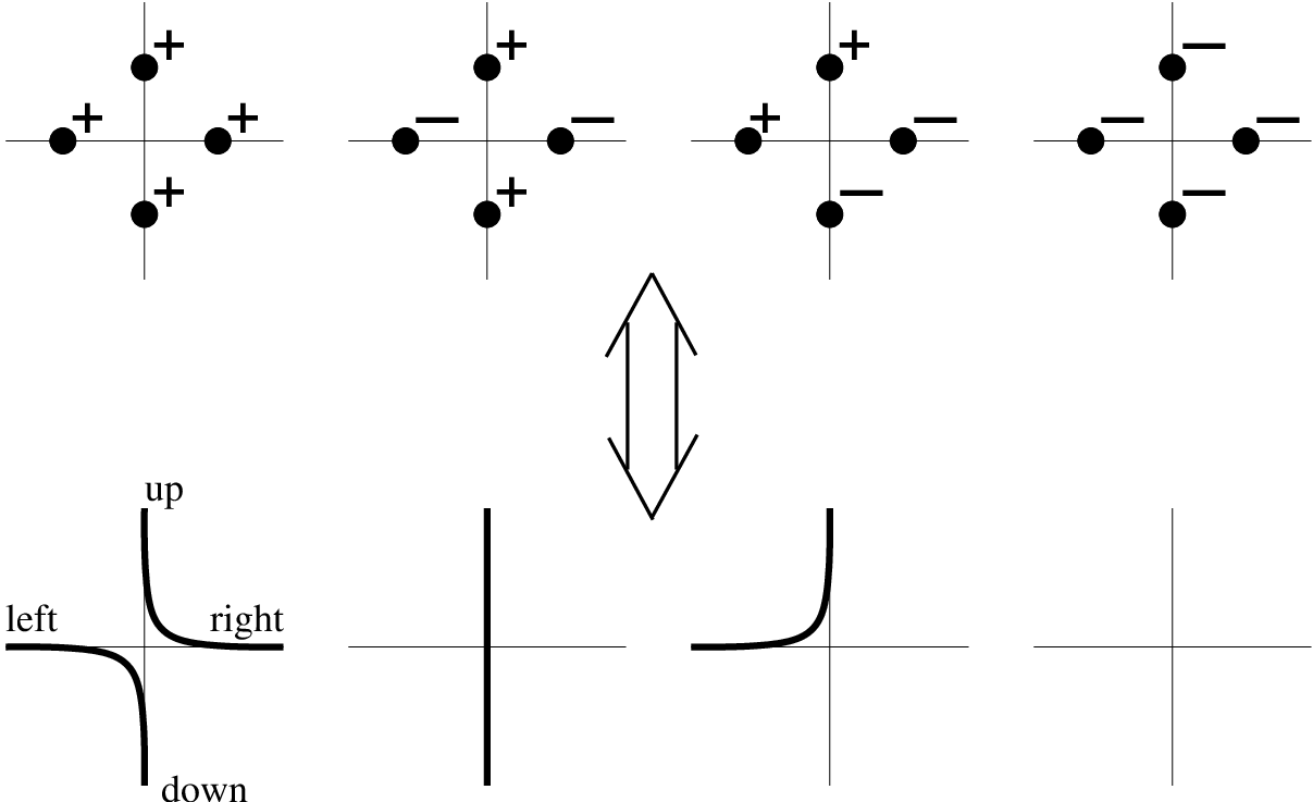
based on the bipartitions shown in Fig. 3.

Refer to caption
Figure 3: Illustration of the four bipartitions used to compute the topological entropy in Ref. Levin2006.

In this specific case, m1​B=2m^{\ }_{1B}=2, with two distinct Σ1​𝒫1\Sigma^{\ }_{1\mathcal{P}^{\ }_{1}} and Σ1​𝒫2\Sigma^{\ }_{1\mathcal{P}^{\ }_{2}} and m2​B=m3​B=m4​B=1m^{\ }_{2B}=m^{\ }_{3B}=m^{\ }_{4B}=1, with a single Σ2​𝒫\Sigma^{\ }_{2\mathcal{P}}, Σ3​𝒫\Sigma^{\ }_{3\mathcal{P}}, Σ4​𝒫\Sigma^{\ }_{4\mathcal{P}}, respectively.

From Eq. (41), it follows that

Stopo​(T)−StopoKitaev\displaystyle S^{\ }_{\textrm{topo}}(T)-S^{\textrm{Kitaev}}_{\textrm{topo}} =\displaystyle= ∑i=12(x~i(1)​ln⁡x~i(1))​cosh⁡(KA2​(N−Σ1​𝒫i))cosh⁡(KA2​N)+∑i=12(y~i(1)​ln⁡y~i(1))​sinh⁡(KA2​(N−Σ1​𝒫i))cosh⁡(KA2​N)\displaystyle\sum^{2}_{i=1}\left(\tilde{x}^{(1)}_{i}\ln\tilde{x}^{(1)}_{i}\right)\frac{\cosh\left(\frac{K^{\ }_{A}}{2}(N-\Sigma^{\ }_{1\mathcal{P}^{\ }_{i}})\right)}{\cosh\left(\frac{K^{\ }_{A}}{2}N\right)}+\sum^{2}_{i=1}\left(\tilde{y}^{(1)}_{i}\ln\tilde{y}^{(1)}_{i}\right)\frac{\sinh\left(\frac{K^{\ }_{A}}{2}(N-\Sigma^{\ }_{1\mathcal{P}^{\ }_{i}})\right)}{\cosh\left(\frac{K^{\ }_{A}}{2}N\right)} (57)
−(x~(2)​ln⁡x~(2))​cosh⁡(KA2​(N−Σ2​𝒫))cosh⁡(KA2​N)−(y~(2)​ln⁡y~(2))​sinh⁡(KA2​(N−Σ2​𝒫))cosh⁡(KA2​N)\displaystyle-\left(\tilde{x}^{(2)}_{\ }\ln\tilde{x}^{(2)}_{\ }\right)\frac{\cosh\left(\frac{K^{\ }_{A}}{2}(N-\Sigma^{\ }_{2\mathcal{P}})\right)}{\cosh\left(\frac{K^{\ }_{A}}{2}N\right)}-\left(\tilde{y}^{(2)}_{\ }\ln\tilde{y}^{(2)}_{\ }\right)\frac{\sinh\left(\frac{K^{\ }_{A}}{2}(N-\Sigma^{\ }_{2\mathcal{P}})\right)}{\cosh\left(\frac{K^{\ }_{A}}{2}N\right)}
−(x~(3)​ln⁡x~(3))​cosh⁡(KA2​(N−Σ3​𝒫))cosh⁡(KA2​N)−(y~(3)​ln⁡y~(3))​sinh⁡(KA2​(N−Σ3​𝒫))cosh⁡(KA2​N)\displaystyle-\left(\tilde{x}^{(3)}_{\ }\ln\tilde{x}^{(3)}_{\ }\right)\frac{\cosh\left(\frac{K^{\ }_{A}}{2}(N-\Sigma^{\ }_{3\mathcal{P}})\right)}{\cosh\left(\frac{K^{\ }_{A}}{2}N\right)}-\left(\tilde{y}^{(3)}_{\ }\ln\tilde{y}^{(3)}_{\ }\right)\frac{\sinh\left(\frac{K^{\ }_{A}}{2}(N-\Sigma^{\ }_{3\mathcal{P}})\right)}{\cosh\left(\frac{K^{\ }_{A}}{2}N\right)}
+(x~(4)​ln⁡x~(4))​cosh⁡(KA2​(N−Σ4​𝒫))cosh⁡(KA2​N)+(y~(4)​ln⁡y~(4))​sinh⁡(KA2​(N−Σ4​𝒫))cosh⁡(KA2​N),\displaystyle+\left(\tilde{x}^{(4)}_{\ }\ln\tilde{x}^{(4)}_{\ }\right)\frac{\cosh\left(\frac{K^{\ }_{A}}{2}(N-\Sigma^{\ }_{4\mathcal{P}})\right)}{\cosh\left(\frac{K^{\ }_{A}}{2}N\right)}+\left(\tilde{y}^{(4)}_{\ }\ln\tilde{y}^{(4)}_{\ }\right)\frac{\sinh\left(\frac{K^{\ }_{A}}{2}(N-\Sigma^{\ }_{4\mathcal{P}})\right)}{\cosh\left(\frac{K^{\ }_{A}}{2}N\right)},

where StopoKitaevS^{\textrm{Kitaev}}_{\textrm{topo}} is the topological entropy of the GS of the original toric code, which obtains from the −ln(d𝒜dℬ)/|G|-\ln(d^{\ }_{\mathcal{A}}d^{\ }_{\mathcal{B}})/|G| contribution to SVN𝒜​(T)S^{\mathcal{A}}_{\textrm{VN}}(T). All the contributions from the (x​ln⁡x)(x\ln x) and (y​ln⁡y)(y\ln y) terms cancel since Σ1​𝒜−Σ2​𝒜−Σ3​𝒜+Σ4​𝒜=0\Sigma^{\ }_{1\mathcal{A}}-\Sigma^{\ }_{2\mathcal{A}}-\Sigma^{\ }_{3\mathcal{A}}+\Sigma^{\ }_{4\mathcal{A}}=0 by construction.

For finite systems, the known limiting values are recovered:

Stopo​(T→0)−StopoKitaev\displaystyle S^{\ }_{\textrm{topo}}(T\to 0)-S^{\textrm{Kitaev}}_{\textrm{topo}} →\displaystyle\rightarrow 0\displaystyle 0 (58)
Stopo​(T→∞)−StopoKitaev\displaystyle S^{\ }_{\textrm{topo}}(T\to\infty)-S^{\textrm{Kitaev}}_{\textrm{topo}} →\displaystyle\rightarrow −ln⁡2.\displaystyle-\ln 2. (59)

In the thermodynamic limit L→∞L\to\infty and with r,Rr,R kept constant, all Σα​𝒫i\Sigma^{\ }_{\alpha\mathcal{P}^{\ }_{i}} diverge with the exception of Σ1​𝒫1\Sigma^{\ }_{1\mathcal{P}^{\ }_{1}}, which corresponds to the inner square of size (R−2​r)2(R-2r)^{2}_{\ } in Fig. 3. Thus, Eq. (57) becomes

Stopo​(T)−StopoKitaev\displaystyle S^{\ }_{\textrm{topo}}(T)-S^{\textrm{Kitaev}}_{\textrm{topo}} =\displaystyle= ∑i=12(x~i(1)​ln​x~i(1)+y~i(1)​ln​y~i(1))​e−KA2​Σ1​𝒫i−(x~(2)​ln​x~(2)+y~(2)​ln​y~(2))​e−KA2​Σ2​𝒫\displaystyle\sum^{2}_{i=1}\left(\tilde{x}^{(1)}_{i}\ln\tilde{x}^{(1)}_{i}+\tilde{y}^{(1)}_{i}\ln\tilde{y}^{(1)}_{i}\right)e^{-\frac{K^{\ }_{A}}{2}\Sigma^{\ }_{1\mathcal{P}^{\ }_{i}}}_{\ }-\left(\tilde{x}^{(2)}_{\ }\ln\tilde{x}^{(2)}_{\ }+\tilde{y}^{(2)}_{\ }\ln\tilde{y}^{(2)}_{\ }\right)e^{-\frac{K^{\ }_{A}}{2}\Sigma^{\ }_{2\mathcal{P}}}_{\ } (60)
−(x~(3)​ln​x~(3)+y~(3)​ln​y~(3))​e−KA2​Σ3​𝒫+(x~(4)​ln​x~(4)+y~(4)​ln​y~(4))​e−KA2​Σ4​𝒫\displaystyle-\left(\tilde{x}^{(3)}_{\ }\ln\tilde{x}^{(3)}_{\ }+\tilde{y}^{(3)}_{\ }\ln\tilde{y}^{(3)}_{\ }\right)e^{-\frac{K^{\ }_{A}}{2}\Sigma^{\ }_{3\mathcal{P}}}_{\ }+\left(\tilde{x}^{(4)}_{\ }\ln\tilde{x}^{(4)}_{\ }+\tilde{y}^{(4)}_{\ }\ln\tilde{y}^{(4)}_{\ }\right)e^{-\frac{K^{\ }_{A}}{2}\Sigma^{\ }_{4\mathcal{P}}}_{\ }
=\displaystyle= (x~1(1)​ln⁡x~1(1)+y~1(1)​ln⁡y~1(1))​e−KA2​Σ1​𝒫1+KA2​Σ1​𝒫2−KA2​Σ2​𝒫−KA2​Σ3​𝒫+KA2​Σ4​𝒫\displaystyle\left(\tilde{x}^{(1)}_{1}\ln\tilde{x}^{(1)}_{1}+\tilde{y}^{(1)}_{1}\ln\tilde{y}^{(1)}_{1}\right)e^{-\frac{K^{\ }_{A}}{2}\Sigma^{\ }_{1\mathcal{P}^{\ }_{1}}}_{\ }+\frac{K^{\ }_{A}}{2}\Sigma^{\ }_{1\mathcal{P}^{\ }_{2}}-\frac{K^{\ }_{A}}{2}\Sigma^{\ }_{2\mathcal{P}}-\frac{K^{\ }_{A}}{2}\Sigma^{\ }_{3\mathcal{P}}+\frac{K^{\ }_{A}}{2}\Sigma^{\ }_{4\mathcal{P}}
=\displaystyle= (x~1(1)​ln⁡x~1(1)+y~1(1)​ln⁡y~1(1))​e−KA2​Σ1​𝒫1−KA2​Σ1​𝒫1,\displaystyle\left(\tilde{x}^{(1)}_{1}\ln\tilde{x}^{(1)}_{1}+\tilde{y}^{(1)}_{1}\ln\tilde{y}^{(1)}_{1}\right)e^{-\frac{K^{\ }_{A}}{2}\Sigma^{\ }_{1\mathcal{P}^{\ }_{1}}}_{\ }-\frac{K^{\ }_{A}}{2}\Sigma^{\ }_{1\mathcal{P}^{\ }_{1}},

where we used the fact that

N\displaystyle N =\displaystyle= Σ1​𝒜+Σ1​𝒫1+Σ1​𝒫2\displaystyle\Sigma^{\ }_{1\mathcal{A}}+\Sigma^{\ }_{1\mathcal{P}^{\ }_{1}}+\Sigma^{\ }_{1\mathcal{P}^{\ }_{2}} (61)
=\displaystyle= Σ2​𝒜+Σ2​𝒫\displaystyle\Sigma^{\ }_{2\mathcal{A}}+\Sigma^{\ }_{2\mathcal{P}} (62)
=\displaystyle= Σ3​𝒜+Σ3​𝒫\displaystyle\Sigma^{\ }_{3\mathcal{A}}+\Sigma^{\ }_{3\mathcal{P}} (63)
=\displaystyle= Σ4​𝒜1+Σ4​𝒜2+Σ4​𝒫,\displaystyle\Sigma^{\ }_{4\mathcal{A}^{\ }_{1}}+\Sigma^{\ }_{4\mathcal{A}^{\ }_{2}}+\Sigma^{\ }_{4\mathcal{P}}, (64)

and that

Σ1​𝒜−Σ2​𝒜−Σ3​𝒜+Σ4​𝒜=0\Sigma^{\ }_{1\mathcal{A}}-\Sigma^{\ }_{2\mathcal{A}}-\Sigma^{\ }_{3\mathcal{A}}+\Sigma^{\ }_{4\mathcal{A}}=0 (65)

to substitute

Σ1​𝒫2−Σ2​𝒫−Σ3​𝒫+Σ4​𝒫=−Σ1​𝒫1\Sigma^{\ }_{1\mathcal{P}^{\ }_{2}}-\Sigma^{\ }_{2\mathcal{P}}-\Sigma^{\ }_{3\mathcal{P}}+\Sigma^{\ }_{4\mathcal{P}}=-\Sigma^{\ }_{1\mathcal{P}^{\ }_{1}} (66)

into Eq.(60). Considering that we are eventually interested in taking limit r,R→∞r,R\to\infty (i.e., Σ1​𝒫1≫1\Sigma^{\ }_{1\mathcal{P}^{\ }_{1}}\gg 1), we obtain the asymptotic value

Stopo​(T)−StopoKitaev\displaystyle S^{\ }_{\textrm{topo}}(T)-S^{\textrm{Kitaev}}_{\textrm{topo}} ⟶L→∞\displaystyle\stackrel{{\scriptstyle L\to\infty}}{{\longrightarrow}} −ln⁡2\displaystyle-\ln 2 (67)

for any non-zero value of TT, that is thermal equilibrium at any infinitesimal temperature leads to a finite loss of topological entropy in the thermodynamic limit. In Sec. VI we discuss the implications of this result, and in particular, we propose an interpretation that naturally explains why the topological entropy reduces to precisely half of its zero-temperature value StopoKitaev=2​ln⁡2S^{\textrm{Kitaev}}_{\textrm{topo}}=2\ln 2.

Notice that Eq. (60) is consistent with both the zero-temperature and the infinite-temperature limits, Eqs. (58,59). Notice also that the topological entropy in the L→∞L\to\infty limit becomes a pure function of KA​Σ1​𝒫1/2K^{\ }_{A}\Sigma^{\ }_{1\mathcal{P}^{\ }_{1}}/2, whose shape is illustrated in Fig. 4

Refer to caption
Refer to caption
Figure 4: (Top) Limiting behavior of the entropy difference Eq. (60) in units of ln⁡2\ln 2 in the thermodynamic limit, as a function of KA​Σ1​𝒫1/2K^{\ }_{A}\Sigma^{\ }_{1\mathcal{P}^{\ }_{1}}/2, where KA=−ln⁡[tanh⁡(λA/T)]K^{\ }_{A}=-\ln[\tanh(\lambda^{\ }_{A}/T)] and Σ1​𝒫1∼(R−2​r)2\Sigma^{\ }_{1\mathcal{P}^{\ }_{1}}\sim(R-2r)^{2}_{\ }, the area of the inner square in Fig. 3. Notice the logarithmic scale on the horizontal axis. (Bottom) The same curve represented as a function of T/λAT/\lambda^{\ }_{A}, for three different values of Σ1​𝒫1=20,200,2000\Sigma^{\ }_{1\mathcal{P}^{\ }_{1}}=20,200,2000 (from right to left).

The location of the drop, say when Stopo(T)−StopoKitaev=−(ln2)/2S^{\ }_{\textrm{topo}}(T)-S^{\textrm{Kitaev}}_{\textrm{topo}}=-(\ln 2)/2, is given by

KA2​Σ1​𝒫1≃14.\frac{K^{\ }_{A}}{2}\,\Sigma^{\ }_{1\mathcal{P}^{\ }_{1}}\simeq\frac{1}{4}. (68)

Even for modest partition sizes with Σ1​𝒫1≳100\Sigma^{\ }_{1\mathcal{P}^{\ }_{1}}\gtrsim 100, the drop occurs at rather small temperatures and we can approximate

KA=−ln⁡[tanh⁡(λAT)]≃2​e−2​λAT.K^{\ }_{A}=-\ln\left[\tanh\left(\frac{\lambda^{\ }_{A}}{T}\right)\right]\simeq 2e^{-2\frac{\lambda^{\ }_{A}}{T}}_{\ }. (69)

This in turn gives

Σ1​𝒫1​e−2​λATdrop≃14⟹Tdrop≃λAln⁡(2​Σ1​𝒫1).\Sigma^{\ }_{1\mathcal{P}^{\ }_{1}}e^{-2\frac{\lambda^{\ }_{A}}{T^{\ }_{\textrm{drop}}}}_{\ }\simeq\frac{1}{4}\;\;\;\Longrightarrow\;\;\;T^{\ }_{\textrm{drop}}\simeq\frac{\lambda^{\ }_{A}}{\ln\left(2\sqrt{\Sigma^{\ }_{1\mathcal{P}^{\ }_{1}}}\right)}. (70)

The l.h.s. of the above equation allows for a straightforward interpretation in terms of defects in the underlying electric loop structure. In fact, e−λA/Te^{-\lambda^{\ }_{A}/T}_{\ } controls the density of such defects in the system, and the equation therefore suggests that the drop in topological entropy occurs when the average number of defects inside partition 1​ℬ11\mathcal{B}^{\ }_{1} becomes of order one.

In order to understand the behavior of Stopo​(T)S^{\ }_{\textrm{topo}}(T) at finite temperature and finite system size, notice that the temperature parameter KA=−ln⁡[tanh⁡(β​λA)]K^{\ }_{A}=-\ln[\tanh(\beta\lambda^{\ }_{A})] in Eq. (57) always appears multiplied by an extensive quantity, be it NN or one of the Σ\Sigma’s. It is therefore convenient to make the reasonable assumption that the number of star operators in each subsystem 𝒜1\mathcal{A}^{\ }_{1}, …, 𝒜m𝒜\mathcal{A}^{\ }_{m^{\ }_{\mathcal{A}}}, and ℬ1\mathcal{B}^{\ }_{1}, …, ℬmℬ\mathcal{B}^{\ }_{m^{\ }_{\mathcal{B}}} scales linearly with the total number of star operators NN. Namely, this amounts to increasing uniformly both LL and r,Rr,R while keeping their ratios fixed, thus simply rescaling the bipartitions in Fig. 3. We can then introduce the notation Σ𝒜=N​γ𝒜\Sigma^{\ }_{\mathcal{A}}=N\gamma^{\ }_{\mathcal{A}}, and Σ𝒫i=N​γ𝒫i\Sigma^{\ }_{\mathcal{P}^{\ }_{i}}=N\gamma^{\ }_{\mathcal{P}^{\ }_{i}}, with γ𝒜,γ𝒫i∈(0,1)\gamma^{\ }_{\mathcal{A}},\gamma^{\ }_{\mathcal{P}^{\ }_{i}}\in(0,1), and γ𝒜+∑iγ𝒫i=1\gamma^{\ }_{\mathcal{A}}+\sum^{\ }_{i}\gamma^{\ }_{\mathcal{P}^{\ }_{i}}=1. Recalling the definitions of x~i(α)=cosh⁡(KA​Σα​𝒫i/2)\tilde{x}^{(\alpha)}_{i}=\cosh(K^{\ }_{A}\Sigma^{\ }_{\alpha\mathcal{P}^{\ }_{i}}/2) and y~i(α)=sinh⁡(KA​Σα​𝒫i/2)\tilde{y}^{(\alpha)}_{i}=\sinh(K^{\ }_{A}\Sigma^{\ }_{\alpha\mathcal{P}^{\ }_{i}}/2), one can replace KAK^{\ }_{A} by 𝒦𝒜=KA​N\mathcal{K}^{\ }_{\mathcal{A}}=K^{\ }_{A}N and all other parameters in Eq. (57) become intensive quantities that do not scale with the system size. Temperature and system size are strongly bound together into a single tunable parameter 𝒦𝒜\mathcal{K}^{\ }_{\mathcal{A}} in our system. The thermodynamic limit at zero temperature is singular, in that the behavior of 𝒦𝒜\mathcal{K}^{\ }_{\mathcal{A}} depends on the order of limits.

IV.1 Numerical evaluation of Stopo​(T)S^{\ }_{\textrm{topo}}(T)

The expression for the topological entropy as a function of temperature and system size Eq. (57) is rather lengthy and non-transparent. In this section we illustrate its behavior graphically, by explicitly evaluating Stopo​(T)S^{\ }_{\textrm{topo}}(T) for small systems. In Fig. 5 we present the difference (Stopo​(T)−StopoKitaev)/ln⁡2(S^{\ }_{\textrm{topo}}(T)-S^{\textrm{Kitaev}}_{\textrm{topo}})/\ln 2 as a function of 𝒦𝒜=KA​N\mathcal{K}^{\ }_{\mathcal{A}}=K^{\ }_{A}N, for various system sizes N=103,106,109N=10^{3}_{\ },10^{6}_{\ },10^{9}_{\ }.

Refer to caption
Figure 5: Topological entropy as a function of 𝒦𝒜\mathcal{K}^{\ }_{\mathcal{A}} for increasing system sizes N=103,106,109N=10^{3}_{\ },10^{6}_{\ },10^{9}_{\ }. Notice the complete overlap between the different curves, due to the fact that the topological entropy Eq. (57) becomes a pure function of 𝒦𝒜=KA​N\mathcal{K}^{\ }_{\mathcal{A}}=K^{\ }_{A}N when all Σ\Sigma’s scale linearly with NN. Notice the logarithmic scale on the horizontal axis.

For convenience, we chose the values of rr and RR proportional to N\sqrt{N}, so that the above assumption on the Σ\Sigma’s holds true, and Stopo​(T)S^{\ }_{\textrm{topo}}(T) is a function of 𝒦𝒜\mathcal{K}^{\ }_{\mathcal{A}} only.

In the limit L→∞L\to\infty, the smooth curves collapse identically onto their infinite-temperature value for any non-vanishing temperature, and a singularity arises at T=0T=0.

The location of the drop is given by KA​N≃10K^{\ }_{A}N\simeq 10, from which we obtain

−ln⁡[tanh⁡(λATdrop)]​N\displaystyle-\ln\left[\tanh\left(\frac{\lambda^{\ }_{A}}{T^{\ }_{\textrm{drop}}}\right)\right]N ≃\displaystyle\simeq 10\displaystyle 10
Tdrop\displaystyle T^{\ }_{\textrm{drop}} ≃\displaystyle\simeq λAtanh−1⁡(e−10N).\displaystyle\frac{\lambda^{\ }_{A}}{\tanh^{-1}_{\ }\left(e^{-\frac{10}{N}}_{\ }\right)}. (71)

For large enough system sizes, TdropT^{\ }_{\textrm{drop}} is small and the above equations reduce to

N​e−2​λATdrop≃5⟹Tdrop≃λAln⁡N/5.Ne^{-2\frac{\lambda^{\ }_{A}}{T^{\ }_{\textrm{drop}}}}_{\ }\simeq 5\;\;\;\Longrightarrow\;\;\;T^{\ }_{\textrm{drop}}\simeq\frac{\lambda^{\ }_{A}}{\ln\sqrt{N/5}}. (72)

Once again, the drop occurs when the average number of defects in the system becomes of order one. (This is consistent with the previous result in Eq. (70) since we made here the assumption that all the Σ\Sigma’s, and therefore Σ1​𝒫1\Sigma^{\ }_{1\mathcal{P}^{\ }_{1}} as well, scale linearly with NN).

V The full temperature range

In the regime considered in this paper, finite temperature disrupts the σx\sigma^{\textrm{x}}_{\ }-loop structure gradually for finite size systems until it is completely destroyed. This happens while the σz\sigma^{\textrm{z}}_{\ }-loop structure is fully preserved, and the topological entropy changes overall from 2​ln⁡22\ln 2 to ln⁡2\ln 2 (half of the contribution is lost).

The remaining topological entropy should fade away as temperature is further increased, and one goes to the regime where defects in the σz\sigma^{\textrm{z}}_{\ }-loop structure also start to appear, for a finite energy scale λB\lambda^{\ }_{B}. The temperature scale of the drop in StopoS^{\ }_{\textrm{topo}} from ln⁡2\ln 2 to 00 corresponds to when the distance between defects, ξB∼eλB/T\xi^{\ }_{B}\sim e^{\lambda^{\ }_{B}/T}, becomes comparable to the system size LL. (Or equivalently, the average number of defects in the system becomes roughly of order one – compare with Eq. (70) and (72).)

It is not obvious how to obtain the exact expression for this second step, in contrast with the first step which we calculated exactly in this paper within the preserved σz\sigma^{\textrm{z}}_{\ }-loop limit. Nevertheless, we believe that the physical picture is the simple one (as seen at work in the first drop) that once a handful of defects appear in that σz\sigma^{\textrm{z}}_{\ }-loop structure, the topological entropy will plunge much like in the first drop. Pasting the two pictures together, we have the two-stage drop of the topological entropy sketched in Fig. 1. Clearly, in the limit |λA−λB|→0|\lambda^{\ }_{A}-\lambda^{\ }_{B}|\to 0 the two drops are expected to merge together, and in particular in the thermodynamic limit the topological entropy entirely vanishes for any infinitesimal temperature.

We would like to point out that a notion of fragility in the Kitaev model at finite temperature, in terms of expectation values of toric operators, has been discussed by Nussinov and Ortiz Nussinov2006 within their definition of topological quantum order (based on gauge-like symmetries).

VI Conclusions

We calculated the entanglement entropy exactly for the toric code at finite temperatures, in a regime where there is a broad separation of energy scales between the two couplings in the problem, λA≪λB\lambda^{\ }_{A}\ll\lambda^{\ }_{B}. These couplings, from a ℤ2\mathbb{Z}_{2} gauge theory perspective, correspond to the chemical potentials of electric charges and magnetic monopoles. One can define length scales associated with the separation between these types of defects, ξA,B∼eλA,B/T\xi^{\ }_{A,B}\sim e^{\lambda^{\ }_{A,B}/T}, and for system sizes much smaller than the largest of these two length scales, i.e., L≪ξBL\ll\xi^{\ }_{B}, one of the two loop structures in the system, associated with the σz\sigma^{\textrm{z}}_{\ }-basis, is preserved. This is the regime where magnetic monopoles are not present in the finite size system. In the limit λB→∞\lambda^{\ }_{B}\to\infty, this holds true for any system size. It is in this limit that we obtain the exact result for the entanglement entropy as a function of T/λAT/\lambda^{\ }_{A}.

Within this hard constrained regime, we find that the entanglement entropy is a singular function of temperature and system size, and that the limit of zero temperature and the limit of infinite system size do not commute. The two limits differ by a term that does not depend on the size of the boundary between the partitions of the system into two entangled parts, but instead depends on the topology of the bipartition. We also calculate the mutual information, obtained from the von Neumann entropy by a symmetrization procedure to filter bulk terms at non-zero temperatures and to leave only boundary and topological contributions. Similarly, the difference between the two orders of limits is an 𝒪⁡(1){\cal O}(1) term that is purely topological, depending on the number of disconnected pieces of partitions 𝒜\mathcal{A} and ℬ\mathcal{B}.

We find that one half of the topological entropy is shaved off from its T=0T=0 value as the temperature increases above Tcross(A)∼λA/ln⁡NT^{(A)}_{\rm cross}\sim\lambda^{\ }_{A}/\ln\sqrt{N}. Above this scale, the loop structure associated with the σx\sigma^{\textrm{x}}_{\ }-basis is destroyed, while the one associated with the σz\sigma^{\textrm{z}}_{\ }-basis survives (recall the λB→∞\lambda^{\ }_{B}\to\infty). We argue that a large but finite value of λB\lambda^{\ }_{B} would introduce another scale Tcross(B)∼λB/ln⁡NT^{(B)}_{\rm cross}\sim\lambda^{\ }_{B}/\ln\sqrt{N}, above which the rest of the topological entropy should also vanish.

As these results show, the topological contributions to the von Neumann entropy or equivalently to the topological entropy, are rather fragile for non-zero temperatures. If the thermodynamic limit is taken first, these quantities subside immediately. However, in practice one should focus on physical regimes and not mathematical limits. The reason why these quantities are so fragile is that 𝒪⁡(1){\cal O}(1) defects can destroy them. However, one must realize that the length scale associated to the defect separation grows exponentially as temperature is decreased, and becomes astronomical for temperatures a few hundred times smaller than the energy scales λA,B\lambda^{\ }_{A,B}. Hence, even if these topological contributions to the entanglement entropy technically vanish, they are statistically present in large but laboratory size physical systems.

If one is interested in understanding how robust is the topological order (information) stored in a single finite system, the notion of a statistically non-vanishing topological entropy naturally translates into the presence of a characteristic time scale over which topoogical order is preserved. Such time scale is associated with the Boltzman probability for the appearance of a defect, namely 𝒩e−λA/T\mathcal{N}\,e^{-\lambda^{\ }_{A}/T}_{\ }, where 𝒩\mathcal{N} is the total number of degrees of freedom in the system. In sight of a possible practical use of such topological quantum information, it would therefore be of great importance to compare this persistence time scale with the one associated to the preparation of the system into a topologically ordered state. Preliminary research in that direction can be found in Ref. Hamma2006 and in Ref. Alicki2007.

At a more fundamental level, our results suggest a simple pictorial interpretation of quantum topological order, at least for systems where there is an easy identification of loop structures as in the case here studied. Recall that we start from a zero-temperature system exhibiting quantum topological order associated with the presence of two identical underlying closed-loop structures. In particular, the corresponding topological entropy equals ln⁡D2\ln D^{2}_{\ }, where D=2D=2 is the so-called quantum dimension of the system. By allowing one of the two loop structures to be thermally disrupted, and by raising T→∞T\to\infty while the other loop structure is fully preserved, we arrive at a classical system with a single (therefore classical) underlying loop structure, and exhibiting precisely half of the original topological entropy (ln⁡D\ln D). This is strongly suggestive that (i) the two loops structures contribute equally and independently to the topological order at zero temperature; (ii) each loop structure per se is a classical (non-local) object carrying a contribution of ln⁡D\ln D to the topological entropy; and (iii) the quantum nature of the zero-temperature system resides in the fact that two independent loop structures are allowed to be superimposed and thus coexist in the system. In this sense, our results lead to an interpretation of quantum topological order, at least for systems with simple loop or membrane structures, as the quantum mechanical version of a classical topological order (given by each individual loop structure).

Finally, we would like to comment on the fact that the same 𝒪⁡(1){\cal O}(1) defects that deteriorate the topological entropy of the system should also deteriorate its usefulness for topological quantum computing. A handful of stray unaccounted defects winding and braiding around others that are accounted for in the computational scheme will lead to errors. These defects can be thermally suppressed, if the temperature is small enough and the system not too large, so that unwanted defects have a small probability of appearing in the sample. Thus, quantifying topological entropy at finite temperature and finite system size is meaningful in quantifying, in a statistical sense, the degree with which a physical (finite) system retains topological order.

Although the results presented here were derived in the case of one of the coupling constants being infinite, we have recently been able to extend the calculations to the case where both coupling constants are finite [C. Castelnovo and C. Chamon, in preparation]. The two contributions to the topological entropy due to the underlying gauge structures are shown to behave additively, and indeed the behavior conjectured in Fig. 1 is confirmed.

Acknowledgments

We are grateful to Xiao-Gang Wen for his insightful comments on the loop structure underlying our model, and to Eduardo Fradkin for enlightening discussions. This work is supported in part by the NSF Grant DMR-0305482 (C. Chamon), and by EPSRC Grant No. GR/R83712/01 (C. Castelnovo). C. Castelnovo would like to acknowledge the I2CAM NSF Grant DMR No. 0645461 for travel support, during which part of this work was carried out.

References

  • (1) F. D. M. Haldane, and E. H. Rezayi, Phys. Rev. B 31, 2529 (1985).
  • (2) X.-G. Wen, and Q. Niu, Phys. Rev. B 41, 9377 (1990).
  • (3) X.-G. Wen, Int. J. Mod. Phys. B 4, 239 (1990); Adv. in Phys. 44, 405 (1995); Phys. Rev. B 65, 165113 (2002).
  • (4) D. Arovas, J. R. Schrieffer, and F. Wilczek, Phys. Rev. Lett. 53, 722 (1984).
  • (5) M. Levin, and X.-G. Wen, Phys. Rev. Lett. 96, 110405 (2006).
  • (6) A. Y. Kitaev, and J. Preskill, Phys. Rev. Lett. 96, 110404 (2006).
  • (7) M. Haque, O. Zozulya and K. Schoutens, Phys. Rev. Lett. 98, 060401 (2007).
  • (8) C. Castelnovo and C. Chamon, arXiv:cond-mat/0610316 (2006) – accepted for publication in Phys. Rev. B.
  • (9) A. Y. Kitaev, Ann. Phys. (N.Y.) 303, 2 (2003).
  • (10) A. Hamma and D. A. Lidar, arXiv:quant-ph/0607145v4 (2006).
  • (11) This limit can be obtained, for example, if the thermal bath is not allowed to couple to the individual degrees of freedom but to (local) products of them (namely, the star operators introduced in Sec. II). Such thermal bath has been previously discussed by Trebst et al. [Phys. Rev. Lett. 98, 070602 (2007)] in the thermodynamic limit, and the authors concluded that no finite-temperature quantum phase transition is to be expected, and that one of the two loop strucutures is indeed preserved for any value of the dissipation strength.
  • (12) We are indebted to Xiao-Gang Wen for pointing out to us the possibility of a much richer behavior in higher dimensions, due to the different nature of the loop and membrane structures underlying topological order.
  • (13) A. Hamma, R. Ionicioiu, and P. Zanardi, Phys. Rev. A 71, 022315 (2005).
  • (14) K. G. Wilson, Phys. Rev. D 10, 2445 (1974); R. Balian, J. M. Drouffe, and C. Itzykson, Phys. Rev. D 11, 2098 (1975); E. Fradkin and L. Susskind, Phys. Rev. D 17, 2637 (1978); E. Fradkin and S. Raby, Phys. Rev. D 20, 2566 (1979); L. Susskind, Phys. Rev. D 20, 2610 (1979).
  • (15) Notice that, while the constraint Σ𝒜+∑iΣ𝒫i=N\Sigma^{\ }_{\mathcal{A}}+\sum^{\ }_{i}\Sigma^{\ }_{\mathcal{P}^{\ }_{i}}=N requires at least one of the Σ\Sigma’s to diverge for L→∞L\to\infty, this does not need to be the case for all of them, in general.
  • (16) Z. Nussinov, and G. Ortiz, arXiv:cond-mat/0605316v2 (2006), and arXiv:cond-mat/0702377 (2007).
  • (17) R. Alicki, M. Fannes, and M. Horodecki, J. Phys. A: Math. Theor. 40, 6451 (2007).