Noncommutativity from spectral flow
Abstract
We investigate the transition from second to first order systems. This transforms configuration space into phase space and hence introduces noncommutativity in the former. Quantum mechanically, the transition may be described in terms of spectral flow. Gaps in the energy or mass spectrum may become large which effectively truncates the available state space. Using both operator and path integral languages we explicitly discuss examples in quantum mechanics, (light-front) quantum field theory and string theory.
pacs
11.10.Ef, 11.15.Bt1 Introduction
The last decade has seen a renaissance of the old idea of noncommutative (‘quantised’) space-time [1], triggered by its reappearance in the context of string and M(atrix) theory [2, 3, 4, 5]. Applications (and publications) are numerous as is well documented by the recent reports and texts on noncommutative geometry [6, 7], deformation quantisation [8], noncommutative field theory [9, 10] and possible phenomenological consequences [11] which include noncommutative approaches to gravity [12, 13], the standard model [14], Lorentz violation [15] and the quantum Hall effect [16, 17].
The latter is based on the quantum mechanics of a particle in a plane pierced by a strong magnetic field. Similar to the string theory scenario it is the presence of the magnetic field that entails noncommutativity between the co-ordinates in the plane. This physics and its exposition in the papers [18, 19, 20, 21, 22] are the original inspiration for the present work. Our main focus is the description of noncommutativity as an emergent phenomenon in terms of spectral flow.
In particular, we analyse how commutative spaces become noncommutative in special limits of quantum mechanical theories. The limits to be studied appear initially to be unrelated. However, we will unveil that there are features common to all, and indeed that there is a unifying picture.
Let us outline our approach, using a generic (spectral flow) parameter to characterise the limits in question as . From an action principle point of view, the limits we consider correspond to terms quadratic in time derivatives (‘velocities’) vanishing or being rendered negligible compared to other terms. As the remaining terms are at most linear in time derivatives, so that we move from a second to a first order system. This implies a significant alteration to the theory, as the definition of the conjugate momenta and therefore the Poisson brackets of the theory will be quite different to when .
When we quantise, Poisson brackets are replaced by commutators of operators. In an operator picture we observe that the energy spectrum is –dependent. As we take the limit some portion of states becomes highly excited and decouples from the theory — effectively this spectral flow truncates the available state space. Operators which commute at do so because of cancellations between the various modes of the operators (think of working with the Fourier modes of a scalar field). As some of these modes are decoupled at such cancellations are incomplete and operators may fail to commute. Typically, it is the configuration space (spacetime co-ordinate or field configuration) operators which become noncommutative in the limit, as the spectral flow takes us to a theory where configuration space becomes phase space.
We will also investigate the limit from a functional perspective, where we show that functionals such as the vacuum and transition amplitudes have natural interpretations as in terms of functionals in the first order theory. Here one must carefully take into account changes to the true degrees of freedom (the arguments of functionals) which occur because of the shift from configuration to phase space.
This paper is organised as follows. In section 2 we discuss the quantum mechanics of a particle in a magnetic field. In the limit in which the magnetic field is large compared to the particle mass we observe that co-ordinates become noncommutative. We describe this limit in the operator language as a projection onto the lowest energy level. From a functional perspective we show how to take account of the change from configuration space to phase space, giving explicit examples of the first order limit of second order transition amplitudes. We conclude this section with a discussion of an analogous situation in string theory, where the presence of a strong ‘magnetic’ field leads to an effective lower dimensional noncommutative field theory.
In section 3 we study the nonrelativistic limit of a quantum field theory, in which states of high energy and momentum are decoupled. We see that the second order Klein-Gordon equation becomes the first order Schrödinger equation and show that only particle-number conserving interactions survive the non-relativistic limit.
In section 4 we describe light-front quantum field theory as a limiting transition to quantising on null-planes. Using ‘almost’ light-front co-ordinates we describe the energy spectrum and show that half of the mass shell energies are decoupled in the light-front limit. We then show explicitly how this leads to non-zero commutators of the field with itself, and describe the vacuum functional and time evolution generator in the light-front limit.
We present our conclusion in section 5. The appendices contain some review material on relevant functional integrals.
2 Particle in a strong magnetic field
2.1 Operator approach
Consider a nonrelativistic particle moving in the plane under the influence of a constant magnetic field of magnitude in the -direction. Upon quantisation this is the problem originally solved by Landau in 1930 [23]. The system is described by the standard Lagrangian [24]
| (1) |
The conjugate momenta are
| (2) |
and obey the equations of motion
| (3) |
These imply three conserved quantities , and with the latter two given by
| (4) |
where is the usual cyclotron frequency. The relevance of these two operators in the quantum theory was first noted by Johnson and Lippmann [25].
Upon performing a Legendre transformation the Hamiltonian is found to be
| (5) |
We introduce ladder operators
| (6) | |||||
| (7) |
in terms of which the Hamiltonian may be written as
| (8) |
Obviously this represents a harmonic oscillator in shifted by , as in (4), and free motion in .
As operators, the conserved quantities (4) commute with the Hamiltonian and the kinematical (not conjugate) momenta. Their commutators with the co-ordinate operators are
| (9) | |||||
| (10) | |||||
| (11) |
Eigenstates of the Hamiltonian are labelled by the oscillator (Landau) level and but are infinitely degenerate with respect to ,
| (12) |
as the energy is independent of ,
| (13) |
Note that the level spacing becomes large for . In this case one expects that transitions between Landau levels are strongly suppressed and that any dynamics will be restricted to the lowest level, [18, 20, 22]. The projection onto the latter is given by the operator
| (14) |
In what follows we evaluate the projected commutator, and show that it is nonvanishing. As a preparation we note
| (15) |
The second equality follows from since and since . Similarly,
| (16) |
Now, commutes with the Hamiltonian, and , so
| (17) |
using . So, finally,
| (18) |
We see that the projection onto the lowest energy level results in a non-zero commutator between the (projected) position operators.
The commutator may be explained in a simple fashion [18, 20, 22] by performing the limit (small mass/large field) in the Lagrangian (1). To retain a nontrivial theory we add an arbitrary potential and arrive at the first order Lagrangian
| (19) |
The Poisson bracket or commutator is read off from the first term (the ‘canonical one-form’ [26]) which yields
| (20) |
Hence, the configuration space variables and become a canonical pair and thus define a phase space on which one has the Hamiltonian
| (21) |
with playing the role of the momentum conjugate to (Peierls’ substitution [27, 28]). The Hilbert space of states may be taken to be consisting of wave functions . The emerging picture will be the basis of the following subsection.
2.2 Path integral approach
We have seen that at a classical level a first order theory is obtained simply by deleting the kinetic term in the Lagrangian of the second order theory, though quantum mechanically the limit is somewhat more subtle. In this subsection we will study the limit from a functional viewpoint.
We begin with a typical wave function in the second order theory, say the amplitude describing particle transition from to in time . In the Euclidean path integral language this amplitude is the sum over all paths between the two points weighted with the exponent of the classical (Euclidean) action,
| (22) |
with the Euclidean version of (1) together with a potential . For a review of this and similar constructions see appendices A and B. For clarity we will neglect any dependence. Let and ( and ) be the Hamiltonian and vacuum energy in the second (first) order theory. In this section we will discuss the following operation and show that it gives first order transition amplitudes in the limit of small mass/large ,
| (23) |
There are two points to consider. The first is the subtraction of the vacuum energy and the second the integration over half of the boundary degrees of freedom in the second order theory. In the operator formalism it has been seen that the energy spectrum undergoes a flow which decouples excited states as . In the case of a particle in a magnetic field this constrains the particle to lie in the ground state, that is the lowest Landau level. Strictly, however, even the ground state of this system acquires a divergent energy, ( in the case of ), and this should be subtracted from the Hamiltonian in order to arrive at a meaningful system. This is most clearly seen using the spectral decomposition of the transition amplitude,
| (24) |
where the sum (which represents any combination of discrete and continuous measure) is over all energy eigenvalues of the Hamiltonian and degeneracies of those energy levels [22]. If the eigenvalues flow to infinity as the mass decreases we see that all terms in this series are exponentially damped and in the massless limit this expression is null. If, however, we subtract the vacuum energy from the Hamiltonian then this sum becomes
| (25) | |||||
where . The first term now survives the limit, the caveat being that these manipulations are only well defined in Euclidean space.
Moving on to the second point we consider the integration over half of the degrees of freedom on the ‘boundary’ and . This has a natural interpretation in the second order theory — rather than consider the amplitude for a transition between points and we instead ask for the amplitude for transition between points and for any initial and final values of . Now, as already stated, in the massless limit the operators and form a conjugate pair. In taking the limit from the second order theory, where these variables are independent, we must choose which of and to consider as a co-ordinate and which a momentum. In the first order theory our prescription corresponds to a particular choice of polarisation or (Schrödinger) representation, namely that where we diagonalise the operator .
In general we must choose one linear combination of and to be diagonalised and compute the transition amplitude between eigenstates of these operators. The remaining degrees of freedom should be integrated over at the boundary. In this way the configuration space path integral becomes a phase space path integral in the first order theory. If we choose to represent states in the massless limit by wave functions , then we integrate over all possible values of the momentum and at the boundaries on the left-hand side of (23) (or the right-hand side of (22)) to arrive at
| (26) |
which, upon changing variables , is a standard phase space path integral describing a transition amplitude in the lower dimensional first order theory. We will give explicit examples below.
2.3 Example one: no external potential
A simple example of the above is given by the particle in a magnetic field with no external potential, for which the transition amplitudes in the first order theory are simply
| (27) |
We would like to relate this amplitude to the ‘projected’ transition amplitude in the theory,
| (28) |
We label energy eigenstates by the oscillator level and an eigenvalue of . The projection operator is then written as an integral over the degenerate ground states ,
normalised such that and so . The projected amplitude (28) may then be written
| (29) | |||||
| (30) |
Comparing this with the spectral decomposition of the full transition amplitude (25) we see that the two coincide at large times (if we rotate to Euclidean space). The effect of the projection is to restrict intermediate states of the system to the ground state, so that transition amplitudes do not obtain contributions from excited states.
To calculate the projected amplitude we first derive the explicit form of the ground state wave function. In the above representation this is given by the two conditions
| (31) |
which are respectively plane wave and harmonic oscillator equations. They have the solutions
| (32) |
Using these functions we follow the procedure of the previous subsection, integrating (29) over and , c.f. (23),
| (33) |
recovering, up to an irrelevant normalisation effect, the trivial transition amplitude (27) of the first order theory.
2.4 Example two: harmonic oscillator potential
We now give a non-trivial example of the massless limit. Consider the (Euclidean) action,
| (34) |
Setting we arrive at the Euclidean action of the harmonic oscillator (upon changing variables ) with frequency and mass . The phase space integral which quantises the action is
| (35) |
where the momentum has a free boundary. This result is well known and in this section we will recover it from the massless limit of the quantised second order theory.
For , following (23), we integrate over boundary values of in the transition amplitude,
| (36) |
The integrals are Gaussian and easily computed, the result is
| (37) |
where the determinant factor is given by
| (38) |
and the exponentiated terms are
| (39) | |||||
| (40) |
The sum over behaves as for large and is convergent, although the result is an unenlightening combination of hypergeometric functions which nevertheless gives the expected result as . Rather than detail this we illustrate it by performing the (in this case) equivalent operations of taking and then performing the sum,
| (41) |
Therefore, in the massless limit we find the exponential of
| (42) |
which is the classical Euclidean action of the harmonic oscillator. We now turn to the determinant factor multiplying this exponential, which is divergent and must be regulated before we can take . Zeta-function regularisation gives
| (43) |
up to an and –independent constant prefactor. The limit of the determinant does not exist as there is an essential singularity at . However, as stated in (23), we should subtract the vacuum energy from the Hamiltonian before taking the limit. This subtraction pre-multiplies the transition amplitude by . The vacuum energy for this system is given in [18],
| (44) |
The limit of the product of the determinant factor and exists (at least for ),
| (45) |
In total we therefore find
| (46) |
which is the transition amplitude for the harmonic oscillator, calculated with the vacuum energy subtracted from the Hamiltonian. This provides a non-trivial example of the prescription (23) describing the transition between a second and first order theory.
2.5 A stringy analogue
The particle in a strong magnetic field has a well known counterpart system in string theory (see [29] and references therein). We consider neutral open strings with Dp-branes on which the strings end. The worldsheet action is
| (47) |
Here and describe the geometry of target space. The worldsheet for free strings, parameterised by and , is an infinite strip in the direction with width in . We will consider a flat target space, , and take the two form flux , representing a magnetic field on the brane, to be constant.
The equation of motion and boundary conditions in the directions parallel to the brane are
| (48) |
which have the solution [30]
| (49) |
The commutation relations are
| (50) |
with all others vanishing and where .
There is a low energy limit of this theory which parallels that of the particle case and which we will discuss shortly. First note that there is a noncommutativity inherent in this system before we take any limit. It is straightforward to check using (50) that
| (51) |
for all and whenever and are not both or . This means that in the bulk of target space, away from the branes, spacetime is described by commutative co-ordinates. However, the commutators between endpoints of the string are non-zero,
| (52) |
The ends of the string therefore describe noncommutative co-ordinates on the branes (closed strings are insensitive to this effect and see spacetime as a commutative manifold). Let us now tie this in our to earlier discussions. A low energy limit of this theory [5] may be taken in which the string coupling and metric scale as
| (53) |
with the magnetic field held fixed — so this is a limit in which is strong compared to other fields, as in the particle case. In studying this limit it is sufficient to focus on a pair of co-ordinates so that all metrics and fields become two by two matrices,
| (54) |
In this limit, the commutators (50) behave as
so that in this limit the theory undergoes a spectral flow in which higher energy states of the open string, created by the action of the oscillators , are suppressed by the vanishing of (which corresponds to the field theory limit). The scaling of the metric also decouples closed string states from the theory. We are left with only the lowest energy states in which the degrees of freedom are the end points of the open string. In this limit the endpoint commutation relations (52) become
| (63) |
in analogy to the quantum mechanical commutator (20). Under (53) the first terms of the action (47), second order in derivatives, are suppressed and it is only the boundary terms which survive the limit,
| (64) |
again in direct analogy to the particle action (19). From this action we may immediately recover (63).
This low energy limit therefore describes a spectral flow in which higher excitations of the string are suppressed, and from the action we see that this corresponds to a transition from a second to first order theory, where the degrees of freedom are noncommutative particle-like co-ordinates on the branes. It is in this way that non-commutative field theories arise on the branes as the low energy limit of string theories [31].
3 The nonrelativistic limit
Throughout the remainder of this paper spacetime is dimensional unless otherwise stated. Functional integrals over time dependent fields will be written while integrals over configurations at constant time will be written .
3.1 Free theory
Consider the action of a free relativistic scalar particle given by the bilinear expression
| (65) |
This action describes either a complex scalar field or a real scalar field (where, for example, may be taken to be the positive frequency part of the real field).
In the nonrelativistic limit, all energies and momenta are small compared to the particle mass . Following [32] we define a new field such that
| (66) |
The motivation for this is that a mode carrying kinetic energy , oscillates as . When the kinetic energy is small compared to the definitions (66) factor out the rapid oscillations which are not admissible in a nonrelativistic approximation.
This argument can only hold if we restrict the energy and momentum of the field, so to proceed we work in momentum space. Defining the Fourier transforms of fields and their conjugates by
| (67) |
the action becomes
| (68) |
and one may verify the relations
| (69) |
We now assume that all energies and momenta are small compared to the particle mass ,
| (70) |
from which we obtain the nonrelativistic approximation
| (71) | |||||
We wish to insert this approximation into the action (68). However, it is clear that this is only consistent if we introduce a large momentum cutoff. Clearly, this is quite natural in the relativistic theory where we have to regulate ultra-violet divergences anyhow. Hence, we change variables in (68) and impose cutoffs in both and momentum . For clarity we refer to only a single cutoff with . We may now insert our approximation (71) into the action,
| (72) |
Inverting the Fourier transform we arrive at the nonrelativistic action in co-ordinate space,
| (73) |
where short distance divergences are controlled by the regulated delta function
| (74) |
As we take the cutoff to infinity we arrive at the nonrelativistic action [33]
| (75) |
Unlike (65) this is now linear in the time derivative and hence the nonrelativistic Schrödinger equation,
| (76) |
correctly becomes first order in the time derivative. As a result (and completely analogous to the Dirac field) the Schrödinger matter field does not commute with its conjugate. Rather we read off the commutator from the term, given by times the Poisson bracket,
| (77) |
Both (75) and (77) coincide with the expressions derived in a slightly different way in the recent text [32].
3.2 Particle number
The Schrödinger matter field still describes an (albeit nonrelativistic) many-body theory. However, the different particle number sectors are separated by huge gaps of order so that particle number becomes conserved. Note that this is also true for nonrelativistic bound states which have binding energies satisfying
| (78) |
where is a typical constituent momentum and the bound state mass. Hence, say for a two-particle bound state, we have , so that is close to the 2-particle threshold and hence separated from the one-particle mass-shell by a gap of almost .
The suppression of number changing interactions in the nonrelativistic limit may be seen from an action principle. Reality requires that polynomial interaction terms take one of the forms
| (79) | |||||
| (80) |
Changing to the new fields of (66), and performing a change of variables for each energy integration variable we have
| (81) |
| (82) |
where the integration is over all and . We have suppressed the momentum dependence for clarity, and to make a consistent relativistic approximation we again understand all integrals to be ultra-violet regulated by .
In the nonrelativistic approximation, when all energies are small compared to , we see that the delta function in loses support because of the non-zero multiple of . These are precisely the interactions which do not conserve particle number, or alternatively, which do not conserve nonrelativistic energy. Hence, only actions of the form , which conserve both particle number and nonrelativistic energy, survive the nonrelativistic limit.
3.3 Projection and particle number
We may now ask, for example, how to get from the field to the one-particle sector and the associated Schrödinger wave function ? The answer is well known: if and denote the vacuum and a one-particle state of momentum then, at ,
| (83) |
is the plane wave solution of the single-particle Schrödinger equation for a free nonrelativistic particle.
To proceed on a slightly more formal level we expand the relativistic field operator (specialising to ) in a Fock basis,
| (84) |
with and the Fourier modes obeying . The field operator changes particle number by one unit, and a one particle state with momentum is defined by
| (85) |
Hence, it makes sense to consider the truncated fields
| (86) | |||||
| (87) |
where we have introduced the projections onto vacuum and one-particle sectors, respectively,
| (88) |
and we restrict the range of momentum to in accordance with the nonrelativistic approximation. We then infer the commutator of the projected fields
| (89) |
with the first (second) term obviously acting in the vacuum (one-particle) sector. Projecting onto the former we find
| (90) | |||||
| (91) |
For the square root is approximately unity, and rescaling the fields with we find the following analogue of (18),
| (92) |
The right-hand side is the one dimensional regulated delta function (74) multiplying the projection . Including the rescaling we thus identify and , recovering (77) in the vacuum sector of the nonrelativistic theory.
Note that the projection formalism above is quite reminiscent of the old Tamm-Dancoff idea of truncating in particle number [34, 35]. If we expand the projected fields (86) and (87) we obtain explicitly
| (93) | |||||
| (94) |
which corresponds to a cutoff in particle number, . In other words, one essentially projects onto negative (positive) frequencies or the annihilation (creation) parts of the field, replacing
| (95) |
in the Tamm-Dancoff spirit. However, it seems obvious that this can only be consistent in a nonrelativistic context where energies and momenta are small compared to particle masses; in a relativistically covariant theory any large boost will spoil these scale hierarchies as boosts, being dynamical Poncarè generators [36], neither conserve energy nor particle number. We will briefly come back to these issues in the next section.
3.4 Transition amplitudes
What can we say about the behaviour of quantum amplitudes in the relativistic limit? Such amplitudes are described in the Schrödinger picture by gluing state wave functionals onto the Schrödinger functional which generates time evolution (see appendices A and B),
| (96) |
As described in the appendices the Schrödinger functional is characterised by temporal boundary terms which, in second order theories, depend on both the field and its derivative, reflecting the fact that Cauchy data is required to determine time evolution. In first order theories the boundary terms depend on the field and its conjugate and do not contain time derivatives (which are not required as data). We have seen how the action changes from a second to first order theory in the nonrelativistic limit, so let us now turn to these boundary terms.
A typical relativistic boundary term for a real scalar field, imposing the Dirichlet condition at time is
| (97) |
where is a functional integration variable obeying the boundary condition , is the boundary field and is a regularisation of . As first noted by Stueckelberg [37] (see also [38]) and discussed in detail by Symanzik, [39], placing sources on the boundary leads to divergences in perturbation theory when the field and its ‘image charges’ (which impose the boundary conditions on propagators) are placed at the same point in time — is hence a short time regulator, which may also be seen as a UV regulator of the field momentum propagator (see appendix B).
In terms of the nonrelativistic degrees of freedom the terms (97) may be written, including a rescaling of the boundary data, ,
| (98) |
Transforming to momentum space and imposing a cutoff, we see that the second line of (98) goes like and is hence suppressed in the nonrelativistic limit. As discussed above, this is consistent with expectations because boundary terms in first order theories should not depend on derivatives of the fields. The third line of (98), in momentum space, goes like . Such terms are also absent in first order theories and we see that if we maintain as the largest scale in our theory, this term is also suppressed in the nonrelativistic limit.
We are therefore left with the first line of (98), depending on the fields and not their momenta, with the condition
| (99) |
up to small corrections, implying a mixed boundary condition on the nonrelativistic fields. We will discuss further limits of field theory wave functionals towards the end of the next section.
4 Light-front quantisation
In 1949 Dirac pointed out that, in a relativistically covariant theory, there are several alternative “forms of relativistic dynamics” [36]. In particular, one may postulate field commutators on null planes rather than entirely space-like hypersurfaces leading to light-cone or, somewhat more precisely, light-front quantum field theory. The literature on this subject is vast and we refer the reader to the reviews [40, 41, 42, 43] and the references cited therein.
One of the hopes of studying light-front quantum field theory was indeed that the Tamm-Dancoff approximation of the previous section might become feasible [44, 45] in a relativistic context. This hope was based on the fact that, upon quantising on null-planes, a number of nonrelativistic features seem to arise within a fully relativistic approach. This was first noted by Weinberg in his analysis of the infinite momentum limit of Feynman graphs [46] (see also [47]) and can be made explicit in terms of a 2 Galilei subgroup of the Poincaré group [48, 49]. Among the consequences one finds, for example, a separation of relative and centre-of-mass motion within bound states. Most interesting seems to be the closely related suppression of vacuum fluctuation and pair production effects expressed as the folkloric statement that the light-front vacuum is ‘trivial’ [41, 42, 43]. In what follows we will take a fresh look at the nonrelativistic aspects of light-front field theory in terms of spectral flow.
4.1 Time-slice geometry
Field quantisation on an arbitrary hypersurface (with time-like or light-like normals) may be formulated as follows [43]. We introduce a coordinate transformation (and likewise for momenta, ),
| (100) |
The new variables describe an alternative (3+1)-foliation of Minkowski space with being the new time variable, conjugate to the momentum component . We assume that the transformation is linear11 1 Clearly, this is not the most general case. Even in special relativity one can choose hyperboloids rather than planes as surfaces of equal time which corresponds to Dirac’s ‘point-form’ of relativistic dynamics [36]. so that
| (101) |
is a hyperplane of equal time . The metric associated with the transformation (100) is
| (102) |
where we have introduced a (3+1)-split in the last step. Hence, is the induced metric on the quantisation hyperplane. The (constant) normal on is
| (103) |
and prominently enters the inverse metric which we write as follows,
| (104) |
The square of the normal can be expressed in terms of metric determinants from (102),
| (105) |
and will become important in a moment. The inverse metric (104) governs the mass-shell constraint,
| (106) |
which will be used to determine the energy variable in terms of the ‘spatial’ components , . We mention in passing that introducing the space-time foliation can be viewed as gauge-fixing the time reparametrisation invariance generated by the constraint (106). The associated Faddeev-Popov (FP) expression is [43]
| (107) |
which has to be evaluated on mass-shell, i.e. by expressing and in terms of and , respectively via (106). Expanding the latter we find the quadric
| (108) |
Interestingly, its discriminant basically coincides with the FP expression squared,
| (109) |
Depending on the value of , we thus have to consider two different cases. The generic one is that the normal on is time–like, . In this case, the mass–shell constraint is of second order in , so that there are two distinct solutions,
| (110) |
The second case to be considered is in a sense degenerate. It corresponds to a light–like normal, . In this case, the constraint (108) is only of first order in leading to a single solution,
| (111) |
with according to (107). While (111) looks simpler than (110) (unique sign, no square root) a new difficulty arises as the momentum projection may be vanishing. We thus have a Gribov problem which will turn into the notorious zero mode problem of light-front field theory.
In what follows we want to study the light-like limit (LLL), .
4.2 The LLL metric
To the best of our knowledge a limiting approach to light-front coordinates was first suggested by Chen in 1971 [50]. His new coordinates differed from light-front ones by an infinitesimal rotation. Finite rotations were later considered in [51, 52].
Clearly, rotations preserve the orthogonality of the coordinates. For relativistic systems this is not a crucial issue, however, and one may as well give up orthogonality. This approach was first adopted by Prokhvatilov and Franke [53] and independently by Lenz et al. [54]. Since then it has frequently been utilised for field theory applications both at zero and finite temperature (see e.g. [55, 56, 57] and [58, 59], respectively). It has also been adopted for the matrix model approach to M-theory [60] where the notion of the ‘LLL’ was coined. The idea is to introduce the new coordinates
| (112) |
such that, in the limit , becomes the standard light-front time,
| (113) |
The invariant distance element is
| (114) |
implying the following metric and its inverse
| (115) |
which we will henceforth refer to as the LLL metric. Comparing with (104) we read off that the hyperplane normal on satisfies
| (116) |
implying that is time-like for . In accordance with that, the line element on is space-like even for vanishing transverse separation,
| (117) |
Hence, for , is indeed a space-like hyperplane.
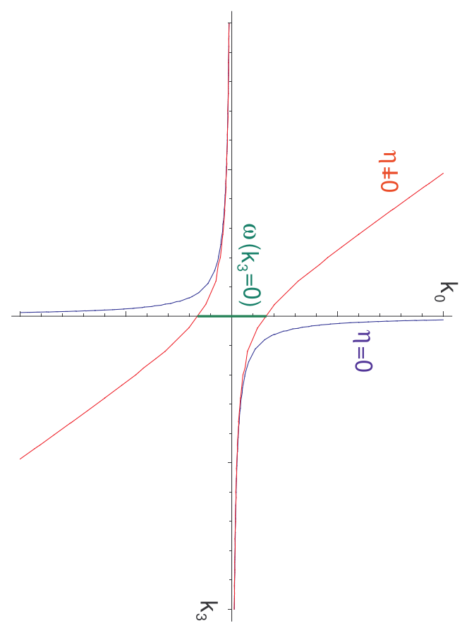
Figure 1 shows the mass shell energy-momentum relation (106) in our co-ordinates (112) and in light-front co-ordinates. The on-shell energies at are
| (118) |
The difference between these two energies will be denoted ,
| (119) |
where is the size of the gap in the energy spectrum of figure 1. Expanding the on-shell energies,
| (120) |
and referring to the four quadrants of figure 1 enumerated anticlockwise from the upper right, we see that the energies in the first and third quadrant remain finite as and become the expected light-front energies, while those in the second and fourth quadrants flow to infinity. In the following subsection we will demonstrate explicitly how this spectral flow gives rise to noncommutativity in the fields.
4.3 Poisson Brackets of the field
A scalar field obeying the LLL co-ordinate equations of motion may be written
| (121) |
Here are the on shell energies (118). The conjugate field momentum is given by
| (122) |
where the first line shows that the momentum contains the velocity only as long as . For , however, is merely an abbreviation for the spatial derivative, . It is easily verified that the equal time Poisson brackets
| (123) | |||||
| (124) |
are equivalent to
| (125) |
with all other brackets vanishing. Referring again to the four quadrants of figure 1, we see that the bracket is non-zero only when one momentum space field has support in the first (second) quadrant and one in the third (fourth). It is precisely the cancellation between these two pairs of sectors which makes the Poisson bracket (124) of the field with itself vanish. This may be verified by splitting the field into two parts, defined by the range of integration over , as so,
| (126) |
These terms live in quadrants one, three, two and four respectively. The contribution from quadrants one and three to the commutator is
| (127) |
while quadrants two and four contribute
| (128) |
which together cancel to give (124). Thus, the commutativity of the fields on hypersurfaces of equal time (expressing relativistic causality) is actually resulting from a delicate ‘interplay’ of different field modes. We will see in a moment that this ‘interplay’ depends crucially on the flow parameter .
So let us now take the limit of vanishing . As terms in corresponding to quadrants one and three have well defined limits, as may be read off from (120). The other terms, however, contain rapidly oscillating complex exponentials since in these quadrants (and on the boundary ) and will be suppressed by said oscillations. Observing that is finite as , , we are left with a truncated field,
| (129) |
where we have written
| (130) |
The momentum space commutator is also well defined in this limit for , ,
| (131) |
and recalculating the Poisson bracket of the field with itself (this may also be read off from the limit of (127)) we find
| (132) |
Thus, we have finally arrived at the canonical Poisson bracket of the light-front field. Again, we see explicitly that spectral flow, causing the decoupling of high-energy states from the theory, alters the Poisson brackets, and therefore the commutators, of the theory. Following the flow all the way to the LLL one goes from a second to a first order theory, thereby inducing a noncommutativity in the configuration space of the original system.
It is useful to work in a mixed representation of light-front theory where the field depends on and by defining, for ,
| (133) |
Using the commutation relations (131) it is easily checked that
| (134) |
So, for all the limit takes us, via spectral flow, to the light-front theory. Note though that our manipulations only hold for , that is off the quantisation hyperplane. Degrees of freedom are eliminated by rapid oscillations only for but remnants survive at in the limit. There are therefore extra degrees of freedom which remain in the quantisation surface and do not propagate into the bulk, . It seems plausible that the boundary degrees of freedom are related to the notorious light-front zero modes (reviewed in [61]) as their propagator is instantaneous, namely proportional to [62] and hence indeed located at the temporal boundary. In the following subsections we will see that the same distinction between bulk and boundary arises in the functional picture.
4.4 Light-front limit of wave functionals - the vacuum
As in previous sections additional insight is provided by studying the behaviour of wave functionals in the light-front limit. We begin with the vacuum wave functional , which may be written as a sum over all field histories beginning in the infinite past and intersecting the configuration at time (see [63], [64], [65] for applications in field theory, string theory and quantum gravity),
| (135) |
where we have rotated to Euclidean space, , and is the (free) Euclidean Lagrangian. The boundary condition at is that the field should be regular.
The integral is computed by splitting into a classical part which obeys the equation of motion and boundary conditions, and a quantum fluctuation which obeys a Dirichlet boundary condition at . The general solution of the equations of motion is
| (136) |
where are the on-shell energies of (118). The boundary conditions of (135) imply that and . The classical and quantum pieces are ‘orthogonal’ in that the action splits into two copies, one evaluated with the above solution and one evaluated with the quantum fields. In this way the integral may be performed to find
| (137) |
with covariance
| (138) |
and where is the contribution of quantum fluctuations. This may be determined from the normalisation condition , which implies
| (139) |
In the limit , the product vanishes for all and tends to for . We therefore find the LLL vacuum wave functional ,
which may be simplified to give
| (140) |
Here we have again transformed to the mixed representation with and . The result (140) coincides with the light-front vacuum wave functional for free scalar fields found in [43]. Some remarks are in order at this point. First, one notes the interesting property that the covariance is local,
| (141) |
unlike the original expression (138) for . Second, both positive and negative longitudinal momenta, , contribute in the exponent. Third, all mass dependence goes away in the LLL, when .
Thus, also from a functional viewpoint we see that the LLL, which we have described in terms of spectral flow (), has drastic effects on the Hilbert space of states. This will be corroborated in the final subsection below.
4.5 Light-front limit of wave functionals - the Schrödinger functional
We now look at the limit of the Schrödinger functional,
| (142) |
Again the integral is performed by splitting the field into orthogonal quantum and classical pieces. Integrating over the quantum fluctuations yields the prefactor , which may be written as the inverse square root of the fluctuation determinant, . Using the standard heat kernel identity
| (143) |
a regulated determinant is defined by inserting a cutoff ,
| (144) |
The classical contribution follows from solving the classical boundary value problem
| (145) |
The general solution (136) now obeys
| (146) |
and it is straightforward to calculate the corresponding action. We find, schematically,
| (147) |
where the asterisks denote convolution integrals. The fields in the mixed representation depend on and and the integral is over all and . The kernels are given by
| (148) |
As we find
| (149) |
where is the light-front energy. The Schrödinger functional (142) therefore becomes, in this limit,
| (150) |
Comparing with (140) the terms in the first line are readily identified with light-front vacuum wave functionals depending on only initial or final fields and , respectively. Hence, with the fields being stuck at and , these terms are non-propagating. The final, -dependent, term, on the other hand, does correspond to propagation being precisely the expression for the anti-holomorphic light-front transition amplitude of appendix A. We may thus write the LLL of the Schrödinger functional (142) in the compact form
| (151) |
Interestingly, one finds a phenomenon that might be called bulk-boundary decoupling: the total transition amplitude decomposes into a product of a bulk and two boundary pieces with the former to be identified with the first-order, light-front transition amplitude proper, . This is consistent with the observation that only half of the original () degrees of freedom survive outside of the quantisation planes as is manifest in that the bulk term contains the propagating modes and with only positive longitudinal momentum, . In Fock space language these modes correspond to creation and annihilation terms corroborating the interpretation that the propagating ’s have indeed become light-front fields.
The bulk-boundary decoupling, with surface modes and , for both positive and negative, attached to the quantisation hypersurfaces, echoes the result of section 4.3 where we saw that the LLL correctly reproduces the light-front commutation relations only off the quantisation surface, i.e. in the bulk.
5 Discussion and conclusions
We have discussed limits of several quantum systems in which second order terms in the action are suppressed. The most striking feature of these limits is that noncommutativity of configuration space appears as an emergent phenomenon resulting from a unifying principle, namely spectral flow. The limits in question may then be described in terms of a generic flow parameter with .
We have seen through various applications that it is the consequential truncation of state space which leads to features of the first order theory which one expects from a naive treatment of the classical action. For example, the change of conjugate momenta to fields rather than their derivatives appears through incomplete cancellations of mode commutators due to missing states, and the expected preservation of particle number in nonrelativistic field theory appears as a restriction on the allowed interactions controlled by the size of the available energy momentum space.
In the functional picture we have examined the Schrödinger and vacuum functionals. In a Schrödinger representation it is only these two objects which are required to build correlation functions and S-matrix elements in perturbation theory. We remark that the form of the boundary terms in the Schrödinger functional, as described by Symanzik [39], are key to understanding renormalisation in the Hamiltonian formalism. This opens up the possibility to interpret the spectral flow presented here as a renormalisation group (RG) flow with the noncommutativity limit corresponding to special RG fixed points. If this is feasible, the difficult renormalisation problem of light-front field theory, for instance, might be attacked from this new vantage point. It is our intention to address this issue in a future publication.
Acknowledgements
The authors are grateful to Andreas Wipf for very useful discussions and A. I. thanks Matthew Daws for helpful correspondence.
Appendix A Transition amplitudes in the anti-holomorphic representation
Given a theory with commutator , where is shorthand for any set of dependent variables, and a Hamiltonian one may describe the abstract space of states by wave functionals of a complex conjugate field, on which the operation of is multiplicative and acts as a derivative,
| (152) |
In this representation the time dependence of physical states is controlled by the Schrödinger equation,
| (153) |
which may be exponentiated to give
| (154) |
The Schrödinger functional, , may be described by a functional integral following the usual procedure of discretising the time interval and inserting complete sets, which are given in this representation by
| (155) |
Note that the measure in this expression is over fields on a constant time hypersurface. The resulting functional integral is
| (156) |
where is the Hamiltonian density. This is the transition amplitude for first order theories derived in the anti-holomorphic representation using coherent states [66]. An equivalent expression, which collects all dependence on the boundary fields into boundary terms in the action, is
| (157) |
This may be derived either by a rearrangement of terms in the discretised product, or in the continuum limit using the change of variables
| (158) |
where the new variables obey . This change of variables corresponds to a separation of degrees of freedom on the boundary, which are fixed by boundary conditions, and in the bulk, which are integrated over.
We will finally give the explicit form of the Schrödinger functional for the (Euclidean) light-front field theory of section 4 where we have commutation relations as in (134),
| (159) |
and Hamiltonian density
| (160) |
The integral in (156) is evaluated by first identifying the solution of the classical equations of motion, which follow from (159) and (160), subject to the boundary conditions , . The integration variable may be decomposed into this field and an orthogonal quantum fluctuation, the integral over the latter giving a determinant factor which stands in need of regularisation. One finds,
| (161) |
with kernel
| (162) |
and light-front energy . As discussed in section 4.5, one may view the light-front theory as the limit of field theory in the LLL metric. We have seen that the functional (161) reappears in this limit as the time dependent (bulk) piece of the LLL Schrödinger functional at .
Appendix B Transition amplitudes in phase space
The representation given above is appropriate for theories with an action which is linear in time derivatives and is analogous to the phase space representation for theories with actions quadratic in time derivatives. Here, using a real scalar field to illustrate, it is common to represent states by wave functionals . We have the algebra , a Hamiltonian density , and complete sets
| (163) |
The Schrödinger functional may be constructed by discretising the time interval and inserting complete sets, where we find
| (164) |
Equivalently,
| (165) |
When the Hamiltonian density is of the form the momentum integration may be carried out to leave a configuration space integral over the exponent of the classical action,
| (166) |
Here is a regularisation of which arises from the UV (short distance) divergent behaviour of the trivial field momentum propagator .
References
References
- [1] H.S. Snyder, Quantized space-time, Phys. Rev. 71, 38 (1947).
- [2] A. Connes, M.R. Douglas and A.S. Schwarz, Noncommutative geometry and matrix theory: Compactification on tori, JHEP 9802, 003 (1998) [arXiv:hep-th/9711162].
- [3] M.R. Douglas and C.M. Hull, D-branes and the noncommutative torus, JHEP 9802, 008 (1998) [arXiv:hep-th/9711165].
- [4] V. Schomerus, D-branes and deformation quantization, JHEP 9906, 030 (1999) [arXiv:hep-th/9903205].
- [5] N. Seiberg and E. Witten, String theory and noncommutative geometry, JHEP 9909, 032 (1999) [arXiv:hep-th/9908142].
- [6] A. Connes, Noncommutative geometry, Academic Press, 1994.
- [7] J. Madore, An Introduction To Noncommutative Differential Geometry And Physical Applications, Cambridge University Press, 1999.
- [8] G. Dito and D. Sternheimer, Deformation Quantization: Genesis, Developments and Metamorphoses, arXiv:math.qa/0201168.
- [9] M.R. Douglas and N. A. Nekrasov, Noncommutative field theory, Rev. Mod. Phys. 73, 977 (2001) [arXiv:hep-th/0106048].
- [10] R.J. Szabo, Quantum field theory on noncommutative spaces, Phys. Rept. 378, 207 (2003) [arXiv:hep-th/0109162].
- [11] I. Hinchliffe, N. Kersting and Y.L. Ma, Review of the phenomenology of noncommutative geometry, Int. J. Mod. Phys. A 19, 179 (2004) [arXiv:hep-ph/0205040].
- [12] P. Aschieri, C. Blohmann, M. Dimitrijevic, F. Meyer, P. Schupp and J. Wess, A gravity theory on noncommutative spaces, Class. Quant. Grav. 22, 3511 (2005) [arXiv:hep-th/0504183].
- [13] P. Aschieri, M. Dimitrijevic, F. Meyer and J. Wess, Noncommutative geometry and gravity, Class. Quant. Grav. 23, 1883 (2006) [arXiv:hep-th/0510059].
- [14] X. Calmet, B. Jurco, P. Schupp, J. Wess and M. Wohlgenannt, The standard model on non-commutative space-time, Eur. Phys. J. C 23, 363 (2002) [arXiv:hep-ph/0111115].
- [15] S.M. Carroll, J. A. Harvey, V. A. Kostelecky, C. D. Lane and T. Okamoto, Noncommutative field theory and Lorentz violation, Phys. Rev. Lett. 87, 141601 (2001) [arXiv:hep-th/0105082].
- [16] L. Susskind, The quantum Hall fluid and non-commutative Chern Simons theory, arXiv:hep-th/0101029.
- [17] S. Hellerman and M. Van Raamsdonk, Quantum Hall physics equals noncommutative field theory, JHEP 0110, 039 (2001) [arXiv:hep-th/0103179].
- [18] G. V. Dunne, R. Jackiw and C. A. Trugenberger, Topological (Chern-Simons) Quantum Mechanics, Phys. Rev. D 41 (1990) 661.
- [19] G. V. Dunne and R. Jackiw, ‘Peierls substitution’ and Chern-Simons quantum mechanics, Nucl. Phys. Proc. Suppl. 33C, 114 (1993) [arXiv:hep-th/9204057].
- [20] Z. Guralnik, R. Jackiw, S. Y. Pi and A. P. Polychronakos, Testing non-commutative QED, constructing non-commutative MHD, Phys. Lett. B 517, 450 (2001) [arXiv:hep-th/0106044].
- [21] R. Jackiw, Physical instances of noncommuting coordinates, Nucl. Phys. Proc. Suppl. 108, 30 (2002) [Phys. Part. Nucl. 33, S6 (2002 LNPHA,616,294-304.2003)] [arXiv:hep-th/0110057].
- [22] R. Jackiw, Observations on noncommuting coordinates and on fields depending on them, Annales Henri Poincare 4S2, S913 (2003) [arXiv:hep-th/0212146].
- [23] L.D. Landau, Diamagnetismus der Metalle, Z. Phys. 64, 629 (1930).
- [24] L.D. Landau and E.M. Lifshitz, The Classical Theory of Fields, Butterworth-Heinemann, 4th revision, 1995.
- [25] M.H. Johnson and B.A. Lippmann, Motion in a Constant Magnetic Field, Phys. Rev. 76, 828, (1949).
- [26] L. D. Faddeev and R. Jackiw, Hamiltonian Reduction of Unconstrained and Constrained Systems, Phys. Rev. Lett. 60, 1692 (1988).
- [27] R. Peierls, Zur Theorie des Diamagnetismus von Leitungselektronen, Z. Phys. 80, 763 (1933).
- [28] C. Duval and P. A. Horvathy, The ”Peierls substitution” and the exotic Galilei group, Phys. Lett. B 479, 284 (2000) [arXiv:hep-th/0002233].
- [29] J. Ambjorn, Y. M. Makeenko, G. W. Semenoff and R. J. Szabo, String theory in electromagnetic fields, JHEP 0302, 026 (2003) [arXiv:hep-th/0012092].
- [30] C. S. Chu and P. M. Ho, Noncommutative open string and D-brane, Nucl. Phys. B 550, 151 (1999) [arXiv:hep-th/9812219].
- [31] R. J. Szabo, Magnetic backgrounds and noncommutative field theory, Int. J. Mod. Phys. A 19, 1837 (2004) [arXiv:physics/0401142].
- [32] A. Zee, Quantum Field Theory in a Nutshell, Princeton University Press, 2003.
- [33] M. A. B. Beg and R. C. Furlong, The Theory in the Nonrelativistic Limit, Phys. Rev. D 31, 1370 (1985).
- [34] I. Tamm, Relativistic Interaction Of Elementary Particles, J. Phys. (USSR) 9, 449 (1945).
- [35] S. M. Dancoff, Nonadiabatic meson theory of nuclear forces, Phys. Rev. 78, 382 (1950).
- [36] P. A. M. Dirac, Forms Of Relativistic Dynamics, Rev. Mod. Phys. 21, 392 (1949).
- [37] E.C.G. Stueckelberg, Relativistic Quantum Theory for Finite Time Intervals, Phys. Rev. 81, 130 (1951).
- [38] N.N. Bogolubov and D.V. Shirkov, Introduction to the theory of quantized fields, Interscience, 1959.
- [39] K. Symanzik, Schrödinger Representation And Casimir Effect In Renormalizable Quantum Field Theory, Nucl. Phys. B 190, 1 (1981).
- [40] J. M. Namyslowski, Light Cone Perturbation Theory And Its Application To Different Fields, Prog. Part. Nucl. Phys. 14, 49 (1985).
- [41] M. Burkardt, Light front quantization, Adv. Nucl. Phys. 23, 1 (1996) [arXiv:hep-ph/9505259].
- [42] S. J. Brodsky, H. C. Pauli and S. S. Pinsky, Quantum chromodynamics and other field theories on the light cone, Phys. Rept. 301, 299 (1998) [arXiv:hep-ph/9705477].
- [43] T. Heinzl, Light-cone quantization: Foundations and applications, Lect. Notes Phys. 572, 55 (2001) [arXiv:hep-th/0008096].
- [44] R. J. Perry, A. Harindranath and K. G. Wilson, Light front Tamm-Dancoff field theory, Phys. Rev. Lett. 65, 2959 (1990).
- [45] R. J. Perry and A. Harindranath, Renormalization in the light front Tamm-Dancoff approach to field theory, Phys. Rev. D 43, 4051 (1991).
- [46] S. Weinberg, Dynamics at infinite momentum, Phys. Rev. 150, 1313 (1966).
- [47] T. Heinzl, Alternative approach to light-front perturbation theory, Phys. Rev. D 75, 025013 (2007) [arXiv:hep-ph/0610293].
- [48] L. Susskind, Model of self-induced strong interactions, Phys. Rev. 165, 1535 (1968).
- [49] K. Bardakci and M. B. Halpern, Theories at infinite momentum, Phys. Rev. 176, 1686 (1968).
- [50] T. W. Chen, Almost-infinite-momentum frame and high-energy scattering processes, Phys. Rev. D 3, 2257 (1971).
- [51] Y. Frishman, C. T. Sachrajda, H. D. I. Abarbanel and R. Blankenbecler, A Novel Inconsistency In Two-Dimensional Gauge Theories, Phys. Rev. D 15, 2275 (1977).
- [52] K. Hornbostel, Nontrivial Vacua From Equal Time To The Light Cone, Phys. Rev. D 45, 3781 (1992).
- [53] E. V. Prokhvatilov and V. A. Franke, Limiting transition of light-front coordinates in field theory and the QCD Hamiltonian, Sov. J. Nucl. Phys. 49, 688 (1989) [Yad. Fiz. 49, 1109 (1989)].
- [54] F. Lenz, M. Thies, K. Yazaki and S. Levit, Hamiltonian formulation of two-dimensional gauge theories on the light cone, Annals Phys. 208, 1 (1991).
- [55] E. V. Prokhvatilov, H. W. L. Naus and H. J. Pirner, Effective light-front quantization of scalar field theories and two-dimensional electrodynamics, Phys. Rev. D 51, 2933 (1995) [arXiv:hep-ph/9406275].
- [56] H. W. L. Naus, H. J. Pirner, T. J. Fields and J. P. Vary, QCD near the light cone, Phys. Rev. D 56, 8062 (1997) [arXiv:hep-th/9704135].
- [57] E. M. Ilgenfritz, S. A. Paston, H. J. Pirner, E. V. Prokhvatilov and V. A. Franke, Quantum Fields on the Light Front, Formulation in Coordinates close to the Light Front, Lattice Approximation, Theor. Math. Phys. 148, 948 (2006) [Teor. Mat. Fiz. 148, 89 (2006)] [arXiv:hep-th/0610020].
- [58] V. S. Alves, A. Das and S. Perez, Light-front field theories at finite temperature, Phys. Rev. D 66, 125008 (2002) [arXiv:hep-th/0209036].
- [59] A. Das and S. Perez, Quantization in a general light-front frame, Phys. Rev. D 70, 065006 (2004) [arXiv:hep-th/0404200].
- [60] S. Hellerman and J. Polchinski, Compactification in the lightlike limit, Phys. Rev. D 59, 125002 (1999) [arXiv:hep-th/9711037].
- [61] K. Yamawaki, Zero-mode problem on the light front, arXiv:hep-th/9802037.
- [62] T. Heinzl, Light-cone zero modes revisited, in: Proceedings of the International Workshop on Light-Cone Physics: Hadrons and Beyond, IPPP/03/71, Durham, 2003; S. Dalley, ed. arXiv:hep-th/0310165.
- [63] A. Jaramillo and P. Mansfield, Finite VEVs from a large distance vacuum wave functional, Int. J. Mod. Phys. A 15, 581 (2000) [arXiv:hep-th/9808067].
- [64] D. Birmingham and C. G. Torre, Functional Integral Construction Of The BRST Invariant String Ground State, Class. Quant. Grav. 4, 1149 (1987).
- [65] J. B. Hartle and S. W. Hawking, Wave Function Of The Universe, Phys. Rev. D 28, 2960 (1983).
- [66] C. Itzykson and J.B. Zuber, Quantum Field Theory, McGraw-Hill, 1980.