Coupling of phonons and spin waves in triangular antiferromagnet

A number of recent experimental breakthroughs has revived interest in the phenomena of coupling between magnetic and electric (dipolar) degrees of freedom in a class of materials known as “multiferroics”review. Some noteworthy observations include the development of dipole moments accompanying the helical spin orderinglawes; kenzelmann, displacement of magnetic ions at the onset of magnetic order in the triangular lattice YMnO₃park, and adiabatic control of dipole moments through applied magnetic fieldskimura; hur, all of which unambiguously point to the strong coupling of electric and magnetic degrees of freedom. A number of theories has been advanced to establish a microscopic understanding of these couplingsKNB; mostovoy; dagotto; harris; JONH; spaldin; jia-han.

The known mechanisms of the spin-polarization coupling fall into two categories. One is of the inverse Dyzaloshinskii-Moriya (DM) type, whereby the local dipole moment, denoted by $u_{ij}$, couples to the spins $S_{i}$ by $\sim u_{ij}\cdot\hat{e}_{ij}\times(S_{i}\times S_{j})$. Here the unit vector $\hat{e}_{ij}$ connects the centers of the magnetic ions at $i$ and $j$. The microscopic origin of such coupling was investigated in, for instance, Refs. KNB; JONH. The behavior of a large class of multiferroic materials can be understood on the basis of this couplingreview. The other type arises from exchange-striction, wherein the movement of the magnetic ions is assumed to directly influence the exchange integral and lead to the coupling $\sim\hat{e}_{ij}\cdot(u_{i}-u_{j})S_{i}\cdot S_{j}$. The spin-lattice coupling in RMn₂O₅ (R=rare earth) is believed to arise from this mechanism125.

More recently, the dynamical aspect of the magnetoelectric coupling has been investigated both experimentallypimenov; drew and theoreticallyKBN. The dynamical coupling is important because it can arise without the ordering of one or both of the degrees of freedom, and can substantially influence the ac dielectric responsepimenov; drew; KBN, or even result in an exotic new phase with vector chiralityonoda-nagaosa. The dynamics of the small fluctuations in the ordered phase of both the polarization and the spin were examined in Ref. KNB for the one-dimensional frustrated chain. A corresponding analysis of the coupled fluctuations has not yet been tried in the case of the exchange-striction mechanism, or for other lattice geometries.

Triangular geometry offers a potentially fertile ground for the interplay of spin and dipolar degrees of freedom because of the tendency of spins to form a spiral ($120{{}^{\circ}}$) structure even without further frustrating interactions. The ground state is characterized by non-zero $\langle S_{i}\cdot S_{j}\rangle$ as well as $\langle S_{i}\times S_{j}\rangle$, which may result in spin-dipole interactions of both DM and exchange-striction types. Furthermore, quite recently, it was shown that a spin $S=5/2$ triangular antiferromagnet in RbFe(MoO₄)₂RFMO develops spontaneous polarization along the $c$ axis as the spins order in the $ab$ plane. This and another triangular lattice compound, YMnO₃, offer promising examples where the interplay of spin and dipolar degrees of freedom can be revealed in detail. In particular, the dynamical aspect of the spin-dipole coupling in the triangular lattice remains largely unexplored and a theoretical consideration of their interplay would be timely.

In this paper, we examine the coupled dynamics of Heisenberg spins and the local dipolar variable (hereafter referred to simply as phonons) on the triangular lattice, assuming the exchange-striction interaction. In Sec. II, the model Hamiltonian is introduced and solved within Holstein-Primakoff theory. A number of physical quantities, such as the local magnetic moment, phonon correlation function, and the dynamic spin-spin correlation, are derived in Sec. III. Conclusions and the relevance of our work to existing experiments can be found in Sec. IV.

The spin-phonon coupled Hamiltonian in the exchange-striction picture readsjia-et-al

where the antiferromagnetic exchange integral $J_{ij}$ connecting the two nearest-neighbor Heisenberg spins is expanded to first order in the displacement $u_{i}$ of each atomic site $i$. $\hat{e}_{ji}$ is the unit vector extending from $i$ to $j$ atomic sites. The terms proportional to $J_{1}$ define the spin-phonon coupling. The Heisenberg spin of magnitude $S$ is represented by $S_{i}$, and the two-dimensional displacement vectors and their canonical conjugate operators by $u_{i}$ and $p_{i}$. We separate the Hamiltonian into two parts, $H=H_{0}+H_{1}$, where $H_{1}$ is the spin-phonon interaction term and $H_{0}$ consists of the Heisenberg and phonon Hamiltonians

The classical ground state of the above Hamiltonian was worked out in Ref. jia-et-al. It was shown that, despite the spin-phonon coupling term, the classical spin configuration is that of the pure Heisenberg model on the triangular lattice with the neighboring spins at a $120^{\circ}$ angle with each other.

Although the spin-phonon interaction does not produce any observable effect in the ground state spin configuration, the excitation spectra of the lattice (phonons) and the spins (magnons) will be mixed due to $H_{1}$.

The small fluctuations near the ground state can be analyzed within the standard Holstein-Primakoff (HP) approach after first rotating the spin operators according to their classical spin orientations defined by $\langle S_{i}\rangle=(0,\sin\phi_{i},\cos\phi_{i})$, where $\phi_{i}$ is the angle the spin makes with the $z$-axis at site $i$. All the spins are assumed to lie in the $yz$-plane, which also coincides with the plane of the lattice itself. After performing the Bogoliubov rotation defined by the angle $\tanh\phi_{k}=3\gamma_{k}/(2+\gamma_{k})$ to obtain the spin wave spectrum, the Hamiltonian $H_{0}$ reads

with the spin wave dispersion

Here $\gamma_{k}=(1/3)\sum_{\alpha=1}^{3}\cos[k\cdot\hat{e}_{\alpha}]$ with $\hat{e}_{1}=(1,0)$, $\hat{e}_{2}=(-1/2,\sqrt{3}/2)$, and $\hat{e}_{3}=(-1/2,-\sqrt{3}/2)$. The lattice constant is taken to unity. Phonon operators in the $y$ and $z$ directions are also introduced above as $b_{ky}$ and $b_{kz}$ as well as the phonon energy $\omega_{0}$.

The spin-phonon Hamiltonian $H_{1}$ can be expanded to second order in the magnon and phonon operators. The full spin-phonon Hamiltonian to quadratic order is given in the simple form ($\overline{k}\equiv-k$)comment

where

Note that only the following linear combination of the phonons participate in the interaction with the magnons:

The rotation of the Hamiltonian to the diagonalized basis is effected by a series of canonical transformations given by $\psi_{k}=W_{k}X_{k}Y_{k}\Psi_{k}$ where $\Psi_{k}$, the diagonal operators, are given by $({\cal A}_{1k},{\cal A}^{\dagger}_{2\overline{k}},{\cal A}_{2k},{\cal A}^{\dagger}_{1\overline{k}})^{T}$. The respective matrices are defined as follows:

where $\Lambda_{k}=\lambda_{k}\cos\theta_{k}$, $\Gamma_{k}=\lambda_{k}\sin\theta_{k}$, $\Delta_{k}=\frac{\Delta_{1k}+\Delta_{2k}}{2}$, $\delta_{k}=\frac{\Delta_{1k}-\Delta_{2k}}{2}$, $\mathcal{E}_{1k,2k}=\sqrt{\Delta_{k}^{2}-\Lambda_{k}^{2}}\pm\delta_{k}$, $E_{1k,2k}=\sqrt{\mathcal{E}_{1k,2k}^{2}-\Gamma_{k}^{2}}$, and $\Delta_{1k,2k}=\frac{\varepsilon_{k}+\omega}{2}\pm\frac{1}{2}\sqrt{(\varepsilon_{k}-\omega)^{2}+4\lambda_{k}^{2}}$. The final form of the Hamiltonian is

The sum $\sum_{k}$ is over the entire Brillouin zone. For any given $k$ we have $E_{1k}\geq E_{2k}$, constituting an upper and lower branch of the spectra.

A plot of $E_{1k}$ and $E_{2k}$ in Fig. 1 shows the change in the magnon and the phonon spectrum as $J_{1}$ is increased. The most notable feature in the coupled energy spectrum is the appearance of the roton-like minimum at a set of $k$-points in the Brillouin zone. When $J_{1}$ equals the threshold value, e.g. $J_{1c}\equiv 0.321$ for $S=1/2$, $\omega_{0}=0.5$, and the phonon wave function width $m\omega_{0}=1$, $E_{2k}$ touches zero at $k=(2\pi,0)$, $(0,2\pi/\sqrt{3})$, and all their sixfold symmetry-related points indicated as white dots in Fig. 1 (c). The original zeros of the magnon spectrum at $\pm(4\pi/3,0)$ remain intact through nonzero $J_{1}$.

As this happens, one has a new spin-ordered pattern illustrated in Fig. 2 becoming degenerate with the original 120^∘ ordered phase. This new pattern is obtained by rotating spins counterclockwise by 120^∘ along the $\hat{e}_{1}$ direction and by 60^∘, also counterclockwise, along the $\hat{e}_{2}$ direction. The state where the spins are rotated clockwise in both directions will also be degenerate, carrying the opposite sense of chirality. In terms of ordering wave vectors, the new ground states are characterized by $Q^{\prime}=\pm(2\pi/3,0)$ instead of $Q=\pm(4\pi/3,0)$ as in the 120^∘ ordered phase.

The local staggered magnetization (uniform magnetization in the rotated basis), $\langle\bm{S}\rangle\equiv(1/N)\sum_{i}\langle\bm{S}_{i}^{z}\rangle$, is modified due to the spin-phonon coupling. The quantum correction, defined as the difference of the classical and quantum averages $S-\langle\bm{S}\rangle$, reads

which is plotted at $T=0$ in Fig. 3 for various spin values as the coupling strength is varied. In small powers of $\lambda_{k}$ one obtains the following perturbative expression as the quantum correction

The first term is the usual quantum fluctuation correction, and the latter two account for further corrections due to spin-phonon coupling. There is only a tiny change in the local magnetization affected by the spin-phonon coupling. On the other hand, the upturn found in Fig. 3 as $J_{1}$ is driven up to its critical value is probably indicative of the diverging quantum correction as the new ground state is approached. Due to the finite phonon mass $\omega_{0}$, the spin-phonon coupling effects are not apparent until very near the criticality.

The equal-time phonon correlation function $\langle{\bf u}_{i}\cdot{\bf u}_{j}\rangle$, which will be short-ranged $\langle{\bf u}_{i}\cdot{\bf u}_{j}\rangle_{0}=\delta_{ij}$ (since we have chosen $m\omega_{0}=1$) in the absence of spin-phonon coupling, now reads

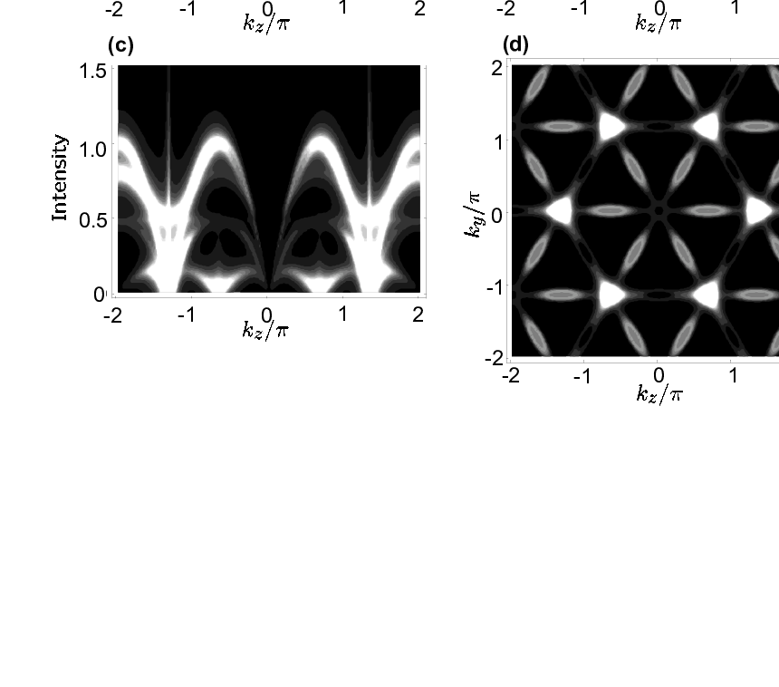
at zero temperature. A log plot of $|\langle{\bf u}_{i}\cdot{\bf u}_{j}\rangle\!-\!\langle{\bf u}_{i}\cdot{\bf u}_{j}\rangle_{0}|$ is given in Fig. 4, showing an exponential decay with a correlation length which depends on the parameters. The momentum space correlation $G_{k}$ shows pronounced peaks around $k=(0,2\pi/\sqrt{3})$ and other symmetry-related points as shown in Fig. 4 (b). These are the same points where $E_{2k}$ shows pronounced minima for large $J_{1}$. Detection of such peaks in the phonon structure factor $G_{k}$ will be instrumental in identifying the spin-phonon coupling in a triangular antiferromagnet.

The spin-spin correlation function, $\langle S_{j}^{+}(t)S_{i}^{-}(0)\rangle$, can be an effective probe of the spin-phonon coupling. Using the straightforward algebra we have calculated the absorption spectra $I(k,\omega)$ as the imaginary part of the Fourier transform of the spin-spin correlation function,

which is plotted in Fig. 5. The functions appearing in Eq. (24) are defined as $k_{1,2}=k\pm(4\pi/3,0)$, and

The flattening and the eventual collapse of the excitation band found earlier now manifests itself as intensity patterns at $(k_{z},k_{y})=(2\pi/3,0)$ and its rotational counterparts as can be seen in Fig. 5 (d).

In summary, we have considered the magnon-phonon coupling in the exchange-striction coupled triangular lattice antiferromagnet for Heisenberg spins in the Holstein-Primakoff approach. The dynamics of the lattice and the spins are coupled to produce interesting modifications in the excitation spectra, in particular (i) the significant lowering of the magnon excitation energy at wave vector transfer $\pm 2\pi$ as indicated in Fig. 1, and (ii) the concordant variation in the phonon structure factor as shown in Fig. 4 (b). Detection of an additional low-energy spectra in the spin spectral function $I(k,\omega)$ and in the phonon structure factor $G_{k}$ through neutron scattering experiments will be a clear hint of the strong spin-phonon coupling.

Naively speaking, integrating out the phonon coordinate from Eq. (1) would generate the effective interaction, $\sim-\sum_{i}(\sum_{j=\textrm{NN of $i$}}\hat{e}_{ij}S_{i}\cdot S_{j})^{2}$, which embodies the ferromagnetic biquadratic exchange, $-(S_{i}\cdot S_{j})^{2}$, and some three-body interactions as well. A quantum spin model involving quadratic and biquadratic exchanges were considered extensivelyspin-nematic following the discovery of the liquid-like ground state in the triangular antiferromagnet NiGa₂S₄nakatsuji1. The ground state revealed correlations, dynamic on the scale of $\sim$ 1 ns, of a period-six spin orientation ($60^{\circ}$ angles between nearest neighbors), quite unlike the period-three orientation ($120^{\circ}$ angles between nearest neighbors) expected in the triangular lattice. It is not easy to reproduce such a spin structure in the mean field solution of the spin models considered in Refs. spin-nematic. In fact, the spin-spin correlation observed in NiGa₂S₄ is almost exactly the one shown in Fig. 2. To correctly account for the observed periodicity of spins in NiGa₂S₄, one would have to consider an extended-neighbor interaction as in Ref. nakatsuji2, or some dynamical consequence of spin-phonon coupling as in the present paper.

We wish to acknowledge fruitful discussions with Chenglong Jia. Discussions with Satoru Nakatsuji on NiGa₂S₄ are also gratefully acknowledged. H. J. H. was partly supported by the Samsung Research Fund, Sungkyunkwan University, 2006.

References

- (1) A recent review of the subject can be found in Y. Tokura, Science 312, 1481 (2006); Sang-Wook Cheong and Maxim Mostovoy, Nature Materials 6, 13 (2007).
- (2) G. Lawes et al., Phys. Rev. Lett. 95, 087205 (2005).
- (3) M. Kenzelmann et al., Phys. Rev. Lett. 95, 087206 (2005).
- (4) Seongsu Lee et al., Phys. Rev. B 71, 180413 (2005).
- (5) T. Kimura, T. Goto, H. Shintani, K. Ishizaka, T. Arima, and Y. Tokura, Nature 426, 55 (2003).
- (6) N. Hur, S. Park, P. A. Sharma, J. S. Ahn, S. Guha, and S.-W. Cheong, Nature 429, 392 (2004).
- (7) Hosho Katsura, Naoto Nagaosa, and Alexander V. Balatsky, Phys. Rev. Lett. 95, 057205 (2006).
- (8) Maxim Mostovoy, Phys. Rev. Lett. 96, 067601 (2006).
- (9) I. A. Sergienko and E. Dagotto, Phys. Rev. B 73, 094434 (2006).
- (10) A. B. Harris, T. Yildirim, A. Aharony, and O. Entin-Wohlman, Phys. Rev. B 73, 184433 (2006).
- (11) Chenglong Jia, Shigeki Onoda, Naoto Nagaosa, and Jung Hoon Han, Phys. Rev. B 74, 224444 (2006); cond-mat/0701614.
- (12) Bas B. van Aken, Thomas T. M. Palstra, Alessio Filippetti, and Nicola A. Spaldin, Nature Materials 3, 164 (2004).
- (13) Chenglong Jia and Jung Hoon Han, Phys. Rev. B 73, 172411 (2006).
- (14) L. C. Chapon et al. Phys. Rev. Lett. 93, 177402 (2004); L. C. Chapon et al. Phys. Rev. Lett. 96, 097601 (2006).
- (15) A. Pimenov et al., Nature Physics 2, 97 (2006).
- (16) A. B. Sushkov et al., Phys. Rev. Lett. 98, 027202 (2007).
- (17) Hosho Katsura, Alexander V. Balatsky, and Naoto Nagaosa, Phys. Rev. Lett. 98, 027203 (2007).
- (18) Shigeki Onoda and Naoto Nagaosa, cond-mat/0703064.
- (19) M. Kenzelman et al. arXiv:cond-mat/0701426 [cond-mat.mtrl-sci].
- (20) Chenglong Jia, Jung Ho Nam, June Seo Kim, and Jung Hoon Han, Phys. Rev. B 71, 212406 (2005).
- (21) Ann Mattsson, Phys. Rev. B 51, 11574 (1995).
- (22) In the unrotated spin basis the phonon at momentum couples to the magnon at , where is the ordering wave vector . Due to the rotation that aligns the spins ferromagnetically, the magnon-phonon coupling appears between the same states.
- (23) Hirokazu Tsunetsugu and Mitsuhiro Arikawa, J. Phys. Soc. Jpn. 75, 083701 (2006); Andreas Läuchli, Frédéric Mila, and Karlo Penc, Phys. Rev. Lett. 97, 087205 (2006); Subhro Bhattacharjee, Vijay B. Shenoy, and T. Senthil, Phys. Rev. B 74, 092406 (2006).
- (24) Satoru Nakatsuji et al. Science 309, 1697 (2005).
- (25) K. Takubo et al. arXiv:0706.2217 [cond-mat.str-el]; To appear in Phys. Rev. Lett.