Boson Propagator Correction in Technicolor Theories with ETC Effects Included
Abstract
We calculate the boson propagator correction, as described by the parameter, in technicolor theories with extended technicolor interactions included. Our method is to solve the Bethe-Salpeter equation for the requisite current-current correlation functions. Our results suggest that the inclusion of extended technicolor interactions has a relatively small effect on .
I Introduction
The origin of electroweak symmetry breaking (EWSB) is an outstanding unsolved question in particle physics. An interesting possibility is that electroweak symmetry breaking is driven by an asymptotically free, vectorial non-abelian gauge interaction, technicolor (TC) tc, with a coupling that becomes strong at the electroweak scale. The EWSB is produced by the formation of bilinear condensates of technifermions. To communicate this symmetry breaking to the standard-model fermions (which are technisinglet), one embeds technicolor in a larger, extended technicolor (ETC) theory etc. In order to account for the generational structure of the standard-model (SM) fermion masses, the ETC gauge symmetry is envisioned to break sequentially in stages at the respective mass scales , , corresponding to these generations, finally yielding the technicolor gauge symmetry as an exact, unbroken subgroup. Because these scales enter as inverse powers in the resultant expressions for quark and lepton masses, the highest ETC symmetry-breaking scale, , corresponds to the first generation, and so forth for the others. The scales and the corresponding masses of the ETC gauge bosons must be large in order to satisfy constraints from flavor-changing neutral current processes. In current, reasonably ultraviolet-complete, ETC models, these ETC breaking scales are TeV, TeV, and few TeV at94-kt. Modern technicolor theories feature a large but slowly running (“walking”) technicolor gauge coupling, wtc1-chipt3. While some early studies of walking assumed an ultraviolet (UV) fixed point in models with U(1) gauge symmetry, modern walking technicolor theories are based on the fact that walking can result naturally from the presence of an approximate infrared (IR) fixed point in the TC renormalization group equations of the non-abelian technicolor gauge theory. This occurs at a value (where ) which is close to, but slightly larger than, the minimal value for which the technifermion condensates form. An important property of a technicolor theory with walking behavior is that the anomalous dimension of the bilinear technifermion operator is , so that the momentum-dependent dynamical technifermion mass falls off as rather than for an extended range of Euclidean momenta . This produces the requisite strong enhancement of SM fermion masses, relative to the values that they would have in a QCD-like (non-walking) theory, which is needed in order to fit experiment. In the pure technicolor theory, the chiral symmetry breaking occurs if exceeds a number of order unity, where denotes the quadratic Casimir invariant for the technifermions, which transform according to the representation of the TC gauge group.
Technicolor theories are severely constrained by the corrections that they induce in precision electroweak quantities, in particular, corrections to the and boson propagators, conveniently represented by the , , and pt or equivalent ab parameters, where and is the deviation of from unity due to new physics beyond the standard model. Experimentally allowed regions in these parameters are given in Refs. pdg. Since the gauge couplings are small at the TeV scale, the condensates of and technifermions can naturally be approximately equal, so that technicolor contributions to are small (e.g., ssvz). Further contributions to may arise from ETC effects, as discussed below. From the point of view of low-energy effective field theory, since the technicolor sector arises as the low-energy residue of the ETC theory, a reasonable first approximation for calculating is to consider the technicolor theory by itself, without any higher-dimension operators arising from ETC interactions. Calculations of this type have been performed in QCD-like and walking technicolor theories pt, scalc-sg (see also adscft; csaki). In particular, it has been found that technicolor contributions to may be suppressed in a TC theory with walking behavior at_s-adscft.
The question then arises as to what influence the exchange of strongly coupled massive ETC gauge bosons, and the resultant effective local four-fermion current-current interaction in the technicolor theory, have on the technicolor correction to the boson propagator, as described by the parameter. Since the ETC gauge coupling is strong at the TeV mass scale, the exchange of the lightest massive ETC vector bosons generates four-fermion operators that could, a priori, have a significant effect on the chiral symmetry breaking in the technicolor theory and on the approximate IR fixed point.
Accordingly, in this paper we study the effects of ETC-induced four-fermion operators on . As a first step, we map out the chiral phase boundary via the solution of a Schwinger-Dyson equation for the technifermion propagator, including both massless technigluon exchange and the leading massive ETC gauge boson exchange. In the context of a walking technicolor model we then solve a Bethe-Salpeter equation for the requisite derivative of the current-current correlation function that yields (cf. eq. (64) below).
The effects of various types of four-fermion operators on dynamical chiral symmetry breaking have been studied in many contexts in the past. In a pioneering work, Nambu and Jona-Lasinio (NJL) showed that a four-fermion operator with a sufficiently strong coupling can induce dynamical chiral symmetry breaking njl. An early approach to nonperturbative generation of fermion masses starting with a massless fermion in electrodynamics (QED) was Ref. jbw. Using large- methods, Ref. gn showed that a certain four-fermion operator in a -dimensional model produced dynamical chiral symmetry breaking. In quantum chromodynamics (QCD) with massless quark flavors, the effective instanton-induced operator is a four-fermion operator hooft, and this was shown to contribute importantly to the formation of a bilinear quark condensate and associated dynamical chiral symmetry breaking qcd_instanton. There have also been studies of the chiral phase transition in both abelian and non-abelian gauge theories with various types of four-fermion operators qed4f-aoki99. We note that the four-fermion operators that we consider are ETC-induced and differ from four-fermion operators directly involving top quark condensates, such as appear in topcolor models.
The paper is organized as follows. Section II is devoted to a review of some pertinent material on technicolor and extended technicolor theories. In Section III we discuss the calculation of the dynamical technifermion mass via the solution of the Schwinger-Dyson equation and the mapping of the chiral phase boundary. Section IV contains the equations expressing in terms of current-current correlation functions. In Section V we discuss our solution of the Bethe-Salpeter equation and our results for . Section VI contains our conclusions. In an appendix we comment on the similarities and differences between the ETC-induced four-fermion interaction that we study and the four-fermion interaction used in the Nambu-Jona Lasino model and its gauged extensions.
II Some Properties of Technicolor and Extended Technicolor Theories
In this section we discuss some properties of the technicolor and extended technicolor theories that will be used in our present study. We begin with the pure technicolor sector and then include ETC. The technicolor theory is a vectorial, asymptotically free gauge theory with a gauge group that we take to have gauge group SU(), with gauge coupling . We choose , as in recent TC/ETC model-building at94-kt, for several reasons, including the fact that this choice (i) minimizes technicolor contributions to the parameter as compared with larger values of , (ii) can naturally produce a walking technicolor theory in a one-family model, and (iii) makes possible a mechanism to explain light neutrino masses nt. To discuss the features of this theory, we shall revert to general for some formulas. The theory contains massless Dirac technifermions, and we assume that these transform according to the fundamental representation of SU() hr. The renormalization group (RG) equation for the running technicolor gauge coupling squared, is
| (1) |
where is the momentum scale, and and are known coefficients. The two terms listed are scheme-independent. The next two higher-order terms have also been calculated but are scheme-dependent; their inclusion does not significantly affect our results. Since the technicolor theory is asymptotically free, . For sufficiently large , , so that the technicolor beta function has a second zero (approximate infrared fixed point of the renormalization group) at a certain , given, to this order, by . As the number of technifermions, , increases, decreases. In a walking technicolor theory, one arranges so that is slightly greater than the critical value, , for the formation of the bilinear technifermion condensate. As increases toward , decreases toward integer. In the one-gluon exchange approximation, the Schwinger-Dyson equation for the inverse propagator of a technifermion transforming according to the representation of the technicolor gauge group yields a nonzero solution for the dynamically generated fermion mass, (which is an order parameter for spontaneous chiral symmetry breaking) if , where is given by
| (2) |
For the case at hand, where the technifermion transforms according to the fundamental representation of SU(), this is , so that, with , . To estimate , one solves the equation , yielding the result chipt2; chipt3 . For this gives . This estimate is clearly rough, in view of the strongly coupled nature of the physics. Moreover, the coupling is only an approximate IR fixed point of the renormalization group, since the technifermions gain dynamical masses and are integrated out in the effective field theory for energies below , where the technicolor beta function consequently has the form for a pure gauge theory. Effects of higher-order gluon exchanges have been studied in alm. From earlier studies in quantum chromodynamics (QCD), it is known that instantons (which are not directly included in the above-mentioned Schwinger-Dyson equation) contribute to the formation of a bilinear fermion condensate in a vectorial gauge theory qcd_instanton. The effect of instantons on the (zero-temperature) chiral transition in a vectorial gauge theory as a function of has been studied in Refs. inst; shuryak. In principle, lattice gauge simulations should provide a way to determine , but the groups that have studied this have not reached a consensus lgt. Thus, we shall use the value for but note that there some uncertainty in the determination of this number, as is expected in view of the strongly coupled nature of the physics.
We shall focus on technicolor models in which the technifermions comprise one family with respect to the standard-model gauge group, (e.g., fs). In such a one-family technicolor model, the technifermions transform as
| (3) | |||
| (4) | |||
| (5) | |||
| (6) | |||
| (7) | |||
| (8) | |||
| (9) | |||
| (10) | |||
| (11) | |||
| (12) | |||
| (13) |
where the numbers in the parentheses refer to the representations of and the subscripts refer to weak hypercharge, . Hence, with , this type of model contains technifermions. Given the above-mentioned fact that , it follows that, to within the accuracy of the two-loop beta function analysis, this technicolor model can naturally exhibit walking behavior. Since there are
| (14) |
SU(2)L doublets for each technicolor index, the total number of electroweak doublets, , of technifermions is
| (15) |
where denotes the technifermion representation of SU(), with here.
We next discuss the embedding of this technicolor theory in extended technicolor. Although much of our analysis of chiral symmetry breaking and the parameter is rather general, it will be useful to have a specific class of ETC models in mind as a theoretical framework. A natural formulation of ETC gauges the fermion generational index and combines it with the technicolor gauge index, so that, for an SU() gauge group, one has
| (16) |
With , this then leads to SU(5) for the ETC gauge group. The SM fermions and corresponding technifermions transform according to the representations
| (17) | |||||
| (19) |
and
| (20) |
where the subscripts denote . For example, writing out the components of , one has , where the last two entries are the charged technileptons. There are also SM-singlet, ETC-nonsinglet fields in various representations of SU(5)ETC such that the overall ETC theory is a chiral gauge theory. The right-handed, SM-singlet, neutrino fields and corresponding technineutrinos arise as certain components of these SM-singlet, ETC representations, as discussed in Refs. at94-kt. In this type of ETC theory, because the SM fermions and the technifermions in each of the ETC multiplets (19) and (20) transform in the same way under the SM gauge group , it follows that the ETC gauge bosons are SM-singlets, and . It may be noted that one could also consider a technicolor theory with a single electroweak doublet of technifermions, so that . Although this model, by itself, does not exhibit walking behavior, this can be achieved by adding the requisite number of SM-singlet technifermions, as, e.g., in ts. To avoid electroweak gauge anomalies, the technifermion electroweak doublet must have weak hypercharge , and consequently, the ETC gauge bosons that transform SM fermions to these technifermions carry hypercharge and charge (and, for some, also color), so that . Consequently, an analysis of electroweak corrections in this type of theory is more complicated than the analysis in a model based on one-family technicolor, and we do not pursue this here.
The overall ETC theory is constructed to be asymptotically free, so that as the energy scale decreases from large values, the ETC gauge coupling grows, and produces various bilinear condensates. Since the ETC theory is chiral, these condensates generically break the ETC gauge symmetry, and this can be arranged to occur in stages. Explicit, reasonably ultraviolet-complete ETC models of this type were studied in Refs. at94-kt. The ETC gauge bosons may be denoted , where . It is convenient to use the notation , for the ETC gauge bosons corresponding to the diagonal Cartan generators . For the sake of generality, we display the for arbitrary . With the canonical normalization and in our basis with ETC indices ordered as for generations and for technicolor, these Cartan generators are
| (21) |
| (22) |
and
| (23) |
where denotes a string of 1’s,
| (24) |
| (25) |
and, most importantly for our purposes,
| (26) |
In particular, for .
At the scale TeV, the SU(5)ETC gauge symmetry is envisioned to break to SU(4)ETC, with the nine ETC gauge bosons in the coset SU(5)ETC/SU(4)ETC, , , , and , picking up masses . Similarly, at the scale TeV, SU(4)ETC breaks to SU(3)ETC, with the seven ETC gauge bosons in the coset SU(4)ETC/SU(3)ETC, , , , and , picking up masses . Finally, at the scale few TeV, SU(3)ETC breaks to the residual exact technicolor gauge group SU(2)TC, and the five ETC gauge bosons in the coset SU(3)ETC/SU(2)TC, , , , and gain masses . Henceforth, we shall denote technicolor indices as to distinguish them from generational indices . In principle, other strongly coupled gauge symmetries such as topcolor might also be present, but we will not consider these here.
The most important ETC contributions to the technicolor sector arise from the exchange of the lowest-lying massive ETC gauge bosons, namely those with mass . Exchanges of more massive ETC gauge bosons make contributions that are strongly suppressed by factors , where . In the technicolor theory, as a low-energy effective field theory, the exchange of massive ETC gauge bosons produce local four-fermion operators of the current-current form. There are two types of corrections to the propagator of a technifermion due to the emission and reabsorption of virtual ETC gauge bosons of mass , namely those involving (i) and (ii) . Thus a one-loop technifermion propagator correction involving the exchange (i) has the same technifermion on the internal fermion line, while that involving the exchange (ii) has the corresponding third-generation SM fermion on the internal line. In a viable ETC model, the exchange (ii) must make a smaller contribution to the dynamical mass of a technifermion than the exchange (i) because it violates custodial symmetry. This is a consequence of the fact that the emission and reabsorption of a virtual yields a one-loop diagram in which a techniquark transforms to a virtual quark and back, while a techniquark transforms to a quark and back. This correction to the dynamical mass of the techniquark therefore introduces a dependence on for and for , so would, in general, differ significantly from , violating custodial symmetry in the technicolor sector.
Such violations must be small. Global fits to data yield allowed regions in depending on a reference value of the SM Higgs mass, . The comparison of these with a technicolor theory is complicated by the fact that technicolor has no fundamental Higgs field. Sometimes one formally uses TeV for a rough estimate, since the standard model with TeV has strong longitudinal vector boson scattering, as does technicolor. However, this may involve some double-counting when one also includes contributions to from technifermions, whose interactions and bound states (e.g., techni-vector mesons) are responsible for the strong scattering in the and other longitudinal vector-vector channels in a technicolor framework. The current allowed region in disfavors values of and pdg.
Because violations of custodial symmetry in the technicolor sector must be small for the theory to be viable, we shall focus on the corrections of type (i). This constraint also implies that , so we shall drop the subscripts on and . Indeed, since all SM interactions are small at the scale of technicolor mass generation, it is expected that the dynamical masses for all of the technifermions, , , , and , are approximately equal, and we shall therefore simply denote them as .
In the ETC framework that we use, the exchange yields an effective local operator in the technicolor theory of the form
| (27) | |||
| (28) | |||
| (29) |
where is over the technifermions in the theory, and is over the technicolor indices. As is evident from eqs. (26) and (29), the dimensionless coefficient is not independent of the technicolor theory and its coupling, , since these arise from the sequential breaking of the ETC theory. However, from an abstract field-theoretic point of view, it is of interest to investigate the (zero-temperature) chiral transition of an asymptotically free vectorial gauge theory in the presence of a four-fermion operator with a coupling that can be varied independently of the gauge coupling. In this context, one could map out the chiral phase boundary as a function of these two, a priori independent, dimensionless couplings. If, indeed, one really posited a four-fermion operator as a fundamental interaction in the theory, it would change the renormalization-group behavior of the couplings. However, in the physical ETC context, in which this four-fermion operator is the low-energy remnant of the ETC theory, its effects on the technicolor gauge coupling can be considered to have already been taken into account at the higher scale where the ETC gauge degrees of freedom are dynamical, since the technicolor sector emerges as the low-energy effective field theory from this larger ETC theory.
By formally varying from zero to its physical nonzero value, and noting that the sign of the resultant contribution to the fermion propagator does not change, one infers that the effect of the ETC interaction is to enhance the spontaneous chiral symmetry breaking. Indeed, the NJL model showed that a four-fermion operator can induce dynamical chiral symmetry breaking by itself if its coupling strength is sufficiently great njl. Note that ETC-induced four-fermion operator (29) is a product of two vector currents and is different from the four-fermion operator that appears in the gauged NJL model, namely a sum of the form , where and denote vector and axial vector currents.
III Schwinger-Dyson Equation and Mapping of Phase Boundary
The first step in our analysis is the calculation of the dynamical technifermion mass and the mapping of the associated chiral phase boundary in the theory. Some early studies using Schwinger-Dyson equations and related methods to study nonperturbative fermion mass generation in abelian and non-abelian gauge theories are Refs. jbw, cjt. Past work on the (zero-temperature) chiral transition for abelian and non-abelian gauge models in the presence of four-fermion operator of various types is contained in Refs. kmy-holdom4f. Several of these studies used models with a (non-asymptotically free) U(1) gauge symmetry. In these studies it was assumed that the theory had a UV fixed point at . This contrasts with modern TC/ETC models, in which the TC sector arises as the low-energy limit of an ETC theory, and both are based on asymptotically free, non-abelian gauge symmetries, with being an approximate IR fixed point of the TC theory.
Our method is to use the Schwinger-Dyson (SD) equation for the technifermion propagator to calculate the dynamically induced mass , taking into account the exchange of both massless technigluons and the massive ETC vector bosons. The dynamical technifermion mass serves as an order parameter for the chiral transition. This mass may be defined in terms of the momentum-dependent fermion mass evaluated at an appropriate Euclidean reference momentum. One choice would be , but we shall actually use the related choice
| (30) |
We recall that the analysis of the Schwinger-Dyson equation, by itself, does not give direct information about whether or not the theory has confinement. Indeed, the original NJL model provides an example of dynamical chiral symmetry breaking via a four-fermion operator (with sufficiently large coupling of the correct sign) without confinement. In the pure gauge theory, for , i.e., for , one can argue persuasively that (although the area law behavior of the Wilson loop ceases to hold because of string breaking) the theory exhibits confinement, by a formal analytic continuation in from integer. This is all that we will need for our present purposes. In the pure gauge theory, the chirally symmetric phase is expected to be a non-abelian deconfined Coulombic phase for sufficiently weak coupling. If appropriate conditions were satisfied, there might possibly also be an intermediate phase with confinement but no spontaneous chiral symmetry breaking; the presence or absence of this phase will not be important for our work here. Since for physical reasons, viz., the necessity of a nonvanishing technifermion condensate for electroweak symmetry breaking, we must be in the confined phase.

The full inverse technifermion propagator can be written as
| (31) |
The resultant SD equation has the form
| (32) |
where and are the contributions from technigluons and ETC vector bosons, respectively. A graphical representation of these contributions is shown in Fig. 1. The first graph on the right is the (massless) technigluon exchange diagram, and the second represents the contribution of the effective local four-fermion operator resulting from the exchange of the massive ETC gauge boson . The dark blobs on the technifermion line signify that we use the full technifermion propagator. The first term in eq. (32) is given by
| (33) |
where the technigluon propagator is
| (34) |
with numerator (depending on the gauge parameter )
| (35) |
Our analysis is thus an improved ladder approximation, where the term “improved” refers to the fact that in eq. (33) we take account of the momentum dependence of the running technicolor coupling, . We next explain several further approximations that will be made. In the pure technicolor theory, if were greater than , i.e., if were less than , so that this IR fixed point of the two-loop RG equation were exact, then one could make use of an exact solution to this equation in the entire energy region. With , this solution is given by gardi; exactsolution
| (36) |
where , with , is the Lambert function, and is a RG-invariant scale defined by chipt2
| (37) |
However, since physically, one must be in the phase where so that the technifermion condensate forms and the electroweak symmetry is broken, the IR fixed point is only approximate rather than exact, as noted above. Hence, eq. (36) is only applicable in an approximate manner to our case; for momenta much less than the dynamical fermion mass , the fermions decouple, and in this very low-momentum region, with the fermions integrated out, the resultant would increase above the value at the approximate IR fixed point. But since in a walking theory, it follows that this lowest range of momenta makes a relatively small contribution to the integrals to be evaluated in our calculations. Hence, over most of the integration range for these integrals where the coupling is large, it is approximately constant and equal to its fixed-point value, . This means that one can use the approximation
| (38) |
where is the step function. Moreover, we shall assume that
| (39) |
Since would naturally depend on the technigluon momentum squared, , the functional form (39) amounts to dropping the scalar product term, . This is a particularly reasonable approximation in the case of a walking gauge theory because most of the contribution to the integral (33) comes from a region of Euclidean momenta where is nearly constant. Hence, the shift upward or downward due to the term in the argument of has very little effect on the value of this coupling for the range of momenta that make the most important contribution to the integral. The approximations (38) and (39) are the same as in our previous work hky_s; s; mmw; pms.
Making a Euclidean rotation and performing the angular integration in then yield two equations, for and . In Landau gauge, with gauge parameter , the solution to the equation for is , so that the dynamical mass of the technifermion, , takes the simple form . This simplification motivates the use of Landau gauge, although physical results involving are, of course, invariant under technicolor gauge transformations (e.g., amnw; alm). For the integral , setting and , we obtain
| (40) |
Note that although the upper limit on the integration is formally infinite, the integral is actually cut off at because of eq. (38). If the technigluon exchange were the only contribution in eq. (32), then this equation would have a nonzero solution for if , where was given by eq. (2). In our calculations, we consider the full nonlinear integral equation (40). However, for comparison with our numerical results, we recall in the pure technicolor theory (without the ETC-induced four-fermion interaction), if, as , one neglects the momentum dependence of in the denominator of eq. (40), then the solution is chipt2-chipt3
| (41) |
A numerical solution of the Schwinger-Dyson equation in a non-abelian gauge theory found a rather similar result, chipt3. A similar numerical solution of the Schwinger-Dyson equation for a range of values of slightly larger than obtained results which were fit with the form (41) mmw.
We next discuss the leading ETC contribution to eq. (32), . We again shall introduce some physically motivated approximations to simplify the calculation. In models with explicit specification of ETC dynamics (e.g., at94-kt), one finds that the walking regime typically extends from the TC scale to the lowest ETC symmetry breaking scale, . Hence, as far as the technicolor theory is concerned, the scale parameter in eq. (37) is of order . At momentum scales , one is dealing with the full SU(3)ETC gauge interaction (and so forth on up to SU(5)ETC for ). Although the dynamical gauge degrees of freedom in the coset are frozen out for momenta , it will be convenient to use the Landau-gauge form of the ETC gauge boson propagator for our calculation, so that
| (42) |
where
| (43) |
This choice maintains . We can then combine the TC and ETC terms as , with
| (44) |
where
| (45) | |||
| (46) | |||
| (47) |
Since the dominant contribution to the momentum integration in is from scales smaller than , the momentum-dependent term in the denominator of the second term (37) is dropped relative to . Since, as noted, the TC sector is the low-energy effective theory arising from ETC, the gauge couplings are closely related. As noted, in explicit ETC models, the walking regime for the TC theory typically extends up to the scale where the ETC symmetry breaks to the TC symmetry. Thus, the approximation (38) for means that the Euclidean momentum integration in the integrals is cut off at . Below this scale, the gauge degrees of freedom in the coset are frozen out, and does not run. Combining this with the fact that the TC gauge coupling inherits its magnitude from the ETC gauge coupling, we will approximate by the same form as , given in eq. (38), namely , with the parameter introduced to account for a slight difference in magnitude between these couplings. We thus obtain (with and )
| (48) |
(Note again that the integral is cut off at because of eq. (38).) From the above, the explicit form for (where ), is
| (49) |
Including the prefactor , we can write this as
| (50) |
where the rescaled coefficient of the ETC-induced four-fermion coupling, , is
| (51) |
With and hence , if , then, taking , the value of the momentum-dependent at the relevant scale of order a TeV, which we shall refer to simply as , is
| (52) |
Thus, the value of in the type of ETC model considered here is rather small.
In addition to ETC-induced four-fermion interactions, certain four-fermion operators could be induced by the nonperturbative dynamics of the technicolor theory itself. In particular, as we discussed above, instanton effects produce effective local multifermion operators, and, upon contraction of technifermion fields, these yield a particular type of four-fermion operator, which has been shown to be important for chiral symmetry breaking in QCD qcd_instanton. These instanton-generated multifermion operators are soft, i.e., the mass that enters as an inverse square factor multiplying them in an effective Lagrangian is of order the QCD chiral symmetry-breaking scale. Indeed, NJL-type four-fermion interactions are commonly used in modern phenomenological models of chiral symmetry breaking in QCD at zero and finite-temperature qcdnjl. Instanton effects on the chiral phase transition depending on have been studied in Refs. inst; shuryak. In Refs. ksy; aoki99 it was suggested that a four-fermion interaction with a strength equivalent to our could be induced by the non-perturbative dynamics of walking technicolor itself. As with instanton-induced multifermion operators, the mass scale characterizing these four-fermion interactions is expected to be . This is different from the type of ETC-induced four-fermion operator considered here, which is hard at the scale (and become soft above ). Although there are no instantons in QED4, the importance of four-fermion operators has also been discussed in connection with a possible UV fixed point in this theory in Ref. qed4f. (This question was relevant to the interpretation of differing results from lattice gauge theory simulations concerning the continuum limit of 4D U(1) lattice gauge theory kogut; schierholz.) If the technicolor theory itself generates large four-fermion operators, then the properties of the theory, even in the absence of ETC effects, might correspond to an interval effectively equivalent to our in the phase diagram of Fig. 7 below. Apart from this, there is also interest, from a general field-theoretic point of view, in investigating the range of values extending up to O(1), where the four-fermion coupling, by itself, would be sufficient to break the chiral symmetry. In accordance with our discussion above, we take to be equal to the scale that effectively sets the upper limit of the walking regime for the technicolor theory.

One next discretizes the Schwinger-Dyson equation and solves it using iterative numerical methods, as described in Ref. mmw (which also contains references to the literature Schwinger-Dyson and Bethe-Salpeter equations). In this analysis, one formally takes and to be independent, although, as discussed above, in the actual ETC context, they are related. In Fig. 2 we show the solution for the dynamical technifermion mass (divided by ) as a function of for a range of values of . The effect of the local current-current interaction is clearly to enhance the spontaneous chiral symmetry breaking, so that the critical value of the technicolor coupling for the appearance of a nonzero , which can be denoted , decreases monotonically as increases from zero. Similarly, if one fixes the value of where is nonzero, then the value of increases monotonically as increases. For , our results are, as expected, in agreement with the exponential vanishing in eq. (41) as decreases toward its critical value, . As increases, this behavior changes. Although the detailed critical behavior as one approaches the chiral boundary is not the focus of our present work, we comment that if one were to make a fit of the form
| (53) |
where is a critical exponent, analogous to the standard notation for the critical exponent for the order parameter in statistical mechanics, then the value of decreases from its value of infinity for , corresponding to the essential zero in eq. (41), through the value at , to the value at .

In Fig. 3 we display contour curves of equal as a function of and . The chiral phase boundary is shown as the dashed curve. For , the critical point for the chiral phase transition is essentially independent of , just as is the case in the gauged NJL model kmy; astw; tak4f. For larger values of , this critical point decreases, and, for , this critical point occurs at , i.e., for , the local current-current interaction is sufficient, by itself, to produce a nonzero , without any technicolor gauge interaction. This is again qualitatively similar to the situation for the gauged NJL interaction.
IV Expression for in Terms of Current-Current Correlation Functions
In this section we review the formulas that we will use to calculate the parameter in terms of (the derivative of) a certain combination of current-current correlation functions. As a measure of corrections to the propagator arising from heavy particles and new physics (NP) in theories beyond the standard model, was originally defined as pt
| (54) |
where , evaluated at . More recent analyses of precision electroweak data define slightly differently, replacing the derivative at by a finite difference (in the scheme) pdg
| (55) |
The difference between these definitions is small if the heavy fermion mass satisfies , as is the case in the technicolor models considered here. To make this quantitative, we recall that in the one-family technicolor model, , where is the SU(2)L coupling and is the technicolor analogue of the pion decay constant in QCD. This yields GeV. We next use a rough scaling relation connecting the dynamical technifermion mass
| (56) |
With MeV, , and , one thus has GeV, so that . For our purposes it will be convenient to use the original definition, Eq. (54).
Suppressing the SU() gauge index, one can write the technifermions as a vector, . One can then define vector and axial-vector currents as
| (57) | |||||
| (59) |
where the matrices () are the generators of with the standard normalization. In terms of these currents, the two-point current-current correlation functions and are defined via the equations
| (60) | |||||
| (62) |
where . Since SM gauge interactions are small at the technicolor scale of several hundred GeV, it follows that the contributions to of each of the techniquark electroweak doublets , and from the technilepton electroweak doublet are essentially equal. It is therefore convenient to define a reduced quantity, , that represents the contribution to from each such technifermion doublet, viz.,
| (63) |
where for the one-family technicolor theory. Then, in terms of the current-current correlation functions defined above, , as defined in Eq. (54), is given by
| (64) |
The relation (64) is equivalent to the expression in terms of the integral over the vector and axial-vector spectral functions for the currents (59) dmo,
| (65) |
where
| (66) |
for .
V Calculation of via Bethe-Salpeter Equation
The method that we use to calculate is similar to our earlier work hky_s; s, except that now we use a scattering kernel for the Bethe-Salpeter equation that includes the exchange of not just the massless technigluons, but also the massive ETC vector boson . We define certain Bethe-Salpeter amplitudes as
| (67) | |||
| (68) | |||
| (69) | |||
| (70) | |||
| (71) |
where or , and , and are, respectively, the flavor, gauge, and spinor indices. In Fig. 4 we show symbolically the terms contributing to the Bethe-Salpeter equation. Full propagators are used on the internal technifermion lines and the running gauge coupling is included.

Closing the fermion legs of the above three-point vertex function and taking the limit , we can express the current-current correlation function in terms of these amplitudes as
| (72) | |||
| (73) | |||
| (74) | |||
| (75) | |||
| (76) |
where
| (77) |
and an average has been taken over the polarizations, so that does not depend on the polarization . We then calculate these amplitudes and evaluate the requisite combination to obtain . Since we include a running coupling in the calculation, we are again working in the improved ladder approximation.
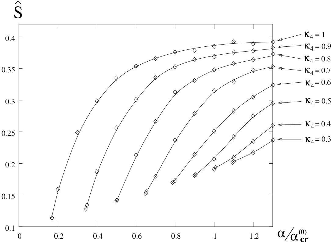
In Fig. 5 we show our results for as a function of for various values of . As in the analysis of the Schwinger-Dyson equation, here again one formally varies and independently, but understands that in a given ETC theory, they are related, via eqs. (51) and (26). For a given value of , the smallest value of is close to ; i.e., the curve starts near to the chiral boundary. For fixed , increases as a function of . This is the same trend that we found in Refs. hky_s; s for the pure gauge theory without four-fermion interaction. For , the reason is clear; as increases, corresponding to a decrease in , one is moving away from the walking regime toward the more QCD-like regime, and the reduction in associated with walking behavior is removed. This increase actually becomes more abrupt as one increases , which indicates that the departure from walking behavior is more abrupt as one moves away from the chiral phase boundary in the presence of a substantial four-fermion coupling. This is in agreement with what we found for the dynamical technifermion mass, namely that as one moves into the chirally broken phase from the chiral phase boundary, the turn-on of is more rapid (i.e., the critical exponent is smaller) for larger values of , as the exponential suppression inherent in the form (41) is removed.


In Fig. 6 we show our results for as a function of for a range of values of . In a walking technicolor theory a typical value of with could be about 1.1. In both Fig. 5 and Fig. 6, the observed feature that increasing at fixed eventually increases is understandable because the current-current interaction facilitates the formation of the technifermion condensate and associated appearance of the dynamical mass . This is the same trend as the increase in that results from increasing (e.g., by decreasing the number of technifermions, ), moving one from the walking regime in the direction of more QCD-like behavior. From inspection of the curve for this value, it is evident that for , with increasing for larger values of . Since is expected to be rather small (cf. eq. (52)), we thus find that in the type of ETC model considered here, the inclusion of the ETC-induced four-fermion operator has little effect on larger. In Fig. 7 we plot curves of constant as functions of and . The chiral boundary is again represented by the dashed curve.

It is also of interest to investigate how behaves if one varies both and (formally taken to be an independent couplings) in such a manner as to move along a contour of a fixed value of the ratio of physical scales . From Fig. 3, it follows that the condition of maintaining fixed means that if one increases , then this should compensated by a decrease in . In models such as those of Ref. ckm-kt, where walking behavior extends up to the lowest ETC breaking scale, , the ratio is typically of order 0.1. The requirement to reduce as much as possible provides motivation to consider a stronger degree of walking and hence a smaller value of . In Fig. 8 we present a plot of for the case where one keeps this ratio fixed at the value . From inspection of Fig. 3, one can see that the contour with intersects the vertical axis at about for , but moves very close to the chiral boundary as increases past 0.4. This is in agreement with the fact that the turn-on of the chiral symmetry-breaking order parameter is more abrupt as increases and the fact that vanishes in the chirally symmetric phase. Our results in Fig. 8 show that decreases as increases, with reduced so as to keep constant. A plausible interpretation of this is that to remain on the contour of fixed as increases, one is moving closer to the chiral boundary. It is also plausible that this decrease in is associated with an increase in the anomalous dimension for the technifermion bilinear . We recall that in the walking limit of a technicolor gauge theory (and for , ). For the expected small value of , our Bethe-Salpeter calculation yields on this contour, so that (using as in eq. (14)). We recall again the possibility that the dynamics of the technicolor theory itself could produce large four-fermion operator effects which could reduce ; here we focus on the ETC-induced contributions. The above value of is too large to agree with experimental limits on , so to maintain the viability of this type of model, it is necessary to assume that there is a further reduction in . We comment on this next.
Although one cannot use perturbation theory reliably to calculate in a strongly coupled gauge theory, the perturbative formula is often employed for comparisons of different technicolor models. The one-loop perturbative calculation with degenerate fermions having effective masses satisfying yields the well-known result where here , so that
| (78) |
In QCD with just light quarks, and hence and hence , this perturbative calculation would predict . To the extent that the experimental value of in QCD is dominated by the contributions of light-quark hadrons in eq. (65) ud, it follows that , so that for QCD. This experimental value of in QCD is svalue, so that the perturbative estimate is about a factor of two smaller than the actual value. An approximate calculation of was carried out using the ladder approximation to the Schwinger-Dyson and Bethe-Salpeter equations for QCD () with quarks of negligible mass hy_s. Studies have also been done for the case where one neglects the strange quark mass , i.e., , hy_s; pms. Since for either of these values of the two-loop beta function of the QCD theory does not exhibit an infrared fixed point, it was necessary in these calculatons to cut off the growth of the strong coupling. For typical cutoffs, it was found that the calculations tended to yield too large a value of , namely hy_s; pms. This suggests that this type of Bethe-Salpeter calculation may overestimate . Our studies of showed that in a walking theory, is reduced, relative to its value in a QCD-like theory hky_s; s, in agreement with other studies of the effect of walkingat_s-iwt_s. Combining this reduction with a plausible correction factor to compensate for the tendency of the Bethe-Salpeter calculation to overestimate in QCD would yield a further reduction in . However, even with a reduction to , inserting the factor yields , which is sufficiently large to be of strong concern. In this context, it should be noted that the question of the value of in walking technicolor has been investigated in recent analyses using holographic methods adscft; csaki, and several authors have found evidence for a a sizable reduction adscft, although Ref. csaki did not. An important task that merits further study is to relate these holographic methods to the sort of Schwinger-Dyson and Bethe-Salpeter methods used in previous works for pure walking gauge theories and here for a walking gauge theory with additional ETC-induced four-fermion interaction.
VI Summary
Technicolor and extended technicolor theories are very ambitious, since they aim to explain not only electroweak symmetry breaking and the associated masses for the and bosons, but also the spectrum of quark, charged lepton, and neutrino masses. A successful model of this type would thus explain longstanding puzzles such as the value of the intergenerational lepton mass ratio and intragenerational mass ratios such as and . It is thus not surprising that no fully realistic ETC model has been constructed. However, since TC/ETC theories continue to provide an interesting theoretical framework complementary to the standard model itself and to other approaches such as supersymmetry, it is worthwhile to investigate their properties further. Accordingly, in this paper, using approximate numerical solutions of the relevant Schwinger-Dyson and Bethe-Salpeter equations, we have calculated the correction to the boson propagator, as described by the parameter, in a technicolor theory, taking account of both massless technigluon exchange and the dominant contribution from massive ETC gauge boson exchange. Our results suggest that for the types of ETC models considered here, this additional contribution from massive ETC gauge boson exchange has a relatively small effect on .
The research of M. K. and R. S. was partially supported by the grant NSF-PHY-03-54776. The research of K. Y. was partially supported by the JSPS Grant-in-Aid for Scientific Research (B) 18340059, and the Mitsubishi and Daiko Foundations. We thank Profs. T. Appelquist and T. Takeuchi for helpful comments.
VII Appendix
It is useful to compare and contrast the ETC-induced four-fermion operator whose effects we have analyzed here with the four-fermion operator studied in the work of Nambu and Jona Lasinio njl and to gauged NJL models. The NJL model for a single fermion is described by the lagrangian , where the interaction term is given by
| (79) | |||||
| (81) |
Here, is a mass scale introduced to make the coupling dimensionless. By a Fierz transformation, this is equivalent to
| (82) | |||||
| (84) |
We define
| (85) |
(This coupling is identical to the coupling in Ref. kmy and to in Ref. astw.) This theory is invariant under a global chiral symmetry group . An analysis of the Schwinger-Dyson equation for the fermion, with an ultraviolet cutoff of imposed on the momentum integration, shows that for , this equation has a nonzero solution for , signifying dynamical chiral symmetry breaking. Associated with this is the formation of a bilinear fermion condensate forms, breaking to the diagonal subgroup . It is straightforward to generalize the model to an -component fermion.
There has also been interest in considering a class of models in which transforms as a nonsinglet under an abelian U(1) or non-abelian SU() gauge group, so that the kinetic term is replaced by , where is the appropriate covariant derivative. In the abelian case, the Fierz transformation relating the interaction in eq. (81) to that in eq. (84) applies in the same manner as for the original NJL model. In the non-abelian case, the situation is more complicated. If the currents in the current-current produce involve the full non-abelian SU() gauge generators, then a Fierz transformation operates not just on the Dirac matrices but also on the matrices representing the gauge generators. As noted in the text, a number of studies of a gauged NJL model, particularly in the abelian case, were performed and mapped out the chiral phase boundary for this type of model as a function of the gauge coupling and the NJL coupling (generically taken to be independent).
There are both similarities and differences between an ETC-based model of the type considered in our text and the non-abelian gauged NJL model. First, the ETC interaction yields a product of two vectorial currents, denoted symbolically as , rather than the structure of the NJL interaction in eq. (84), which is . Second, while the NJL model requires an ultraviolet cutoff, this is not necessary in the present case since we actually start with a reasonably ultraviolet-complete theory, from which the interaction (29) arises as part of the effective low-energy field theory. Third, while the general gauged NJL model treats and the gauge coupling as independent, this is not the case in a TC/ETC theory, since the TC gauge group arises as a subgroup of the ETC gauge group and hence the running TC gauge coupling at a given scale is determined by the ETC gauge coupling at the higher ETC scales where the ETC gauge degrees of freedom are still active.
In an approximation in which the term in the denominator of the fermion propagator is neglected, thereby linearizing the Schwinger-Dyson equation, it was found that, as one increases the NJL coupling from zero, the critical gauge coupling remains unchanged for and, for , the chiral phase boundary can be described by the following functional relation for the coordinates of a point on this boundary,
| (86) |
or equivalently, . As one moves up along the phase boundary from the point to , the nature of the critical singularity also changes from the essential zero in eq. (41) to the algebraic singularity (53) as .
In the gauged NJL model, the Schwinger-Dyson equation is, after Euclidean rotation and angular integration, in the notation of Section III,
| (87) | |||||
| (89) |
If one were formally to replace the factor in our eqs. (48)-(50) by , then the Schwinger-Dyson equation for the ETC model analyzed in the present paper would be transformed into a structure equivalent to that studied in Refs. kmy; astw; tak4f. Since the factor takes the value unity for and and takes the maximal value 2 (at ), one could anticipate that the solutions for the Schwinger-Dyson equation in the present paper should be formally similar to the results obtained in Refs. kmy; astw; tak4f for the same input values of and similar values of and .
References
- (1) S. Weinberg, Phys. Rev. D 19, 1277 (1979); L. Susskind, ibid. D 20, 2619 (1979); see also S. Weinberg, Phys. Rev. D 13, 974 (1976).
- (2) S. Dimopoulos and L. Susskind, Nucl. Phys. B 155, 237 (1979); E. Eichten and K. Lane, Phys. Lett. B 90, 125 (1980).
- (3) T. Appelquist and J. Terning, Phys. Rev. D 50, 2116 (1994).
- (4) T. Appelquist and R. Shrock, Phys. Lett. B 548, 204 (2002); Phys. Rev. Lett. 90, 201801 (2003).
- (5) T. Appelquist, M. Piai, and R. Shrock, Phys. Rev. D 69, 015002 (2004); Phys. Lett. B 593, 175 (2004); ibid. B 595, 442 (2004).
- (6) T. Appelquist, N. Christensen, M. Piai, and R. Shrock, Phys. Rev. D 70, 093010 (2004).
- (7) B. Holdom, Phys. Lett. B 150, 301 (1985).
- (8) K. Yamawaki, M. Bando, and K. Matumoto, Phys. Rev. Lett. 56, 1335 (1986).
- (9) T. Appelquist, D. Karabali, and L. C. R. Wijewardhana, Phys. Rev. Lett. 57, 957 (1986).
- (10) T. Appelquist and L. C. R. Wijewardhana, Phys. Rev. D 35, 774 (1987); Phys. Rev. D 36, 568 (1987).
- (11) M. Bando, T. Morozumi, H. So, and K. Yamawaki, Phys. Rev. Lett. 59, 389 (1987).
- (12) T. Appelquist, K. Lane, and U. Mahanta, Phys. Rev. Lett. 61, 1553 (1988).
- (13) A. Cohen and H. Georgi, Nucl. Phys. B 314, 7 (1989).
- (14) T. Appelquist, J. Terning, and L. C. R. Wijewardhana, Phys. Rev. Lett. 77, 1214 (1996).
- (15) V. Miransky and K. Yamawaki, Phys. Rev. D 55, 5051 (1997); ibid. 56, E 3768 (1997).
- (16) R. S. Chivukula, Phys. Rev. D 55, 5238 (1997).
- (17) T. Appelquist and S. Selipsky, Phys. Lett. B 400, 364 (1997).
- (18) M. Velkovsky and E. Shuryak, Phys. Lett. B 437, 398 (1998).
- (19) T. Appelquist, A. Ratnaweera, J. Terning, and L. C. R. Wijewardhana, Phys. Rev. D 58, 105017 (1998).
- (20) M. Peskin and T. Takeuchi, Phys. Rev. Lett. 65, 964 (1990); M. Peskin and T. Takeuchi, Phys. Rev. D 46, 381 (1992).
- (21) G. Altarelli and R. Barbieri, Phys. Lett. B 253, 161 (1991); G. Altarelli, R. Barbieri, F. Caravaglios, Int. J. Mod. Phys. A 13, 1031 (1998).
- (22) See http://pdg.lbl.gov and http://lepewwg.web.cern.ch.
- (23) P. Sikivie, L. Susskind, M. Voloshin and V. Zakharov, Nucl. Phys. B 173, 189 (1980).
- (24) B. Holdom and J. Terning, Phys. Lett. B 247, 88 (1990); M. Golden and L. Randall, Nucl. Phys. B 361, 3 (1991); H. Georgi, Nucl. Phys. B 363, 301 (1991); R. Johnson, B.-L. Young, and D. McKay, Phys. Rev. D 43, R17 (1991); R. Cahn and M. Suzuki, Phys. Rev. D 44, 3641 (1991);
- (25) T. Appelquist and G. Triantaphyllou, Phys. Lett. B 278, 345 (1992).
- (26) R. Sundrum and S. Hsu, Nucl. Phys. B 391, 127 (1993).
- (27) M. Harada and Y. Yoshida, Phys. Rev. D 50, 6902 (1994).
- (28) T. Appelquist, N. Evans, and S. Selipsky, Phys. Lett. B 374, 145 (1996).
- (29) T. Appelquist and F. Sannino, Phys. Rev. D 59, 067702 (1999).
- (30) S. Ignjatovic, L. C. R. Wijewardhana, and T. Takeuchi, Phys. Rev. D 61, 056006 (2000).
- (31) N. Christensen and R. Shrock, Phys. Rev. Lett. 94, 241801 (2005).
- (32) M. Harada, M. Kurachi, and K. Yamawaki, Prog. Theor. Phys. 115, 765 (2006); see also M. Kurachi, in Proc. of the 2004 Workshop on Dynamical Symmetry Breaking, Dec. 2004, eds. M. Harada and K. Yamawaki (Physics Department, Nagoya University, Nagoya), p. 125.
- (33) M. Kurachi and R. Shrock, Phys. Rev. D 74, 056003 (2006).
- (34) M. Kurachi and R. Shrock, JHEP 12, 034 (2006).
- (35) D. K. Hong and H.-U. Yee, Phys. Rev. D 74, 015011 (2006); J. Hirn and V. Sanz, Phys. Rev. Lett. 97, 121803 (2006); J. Hirn and V. Sanz, JHEP 0703, 100 (2007); M. Piai, hep-ph/0608241.
- (36) K. Agashe, C. Csáki, C. Grojean, and M. Reece, arXiv:0704.1821.
- (37) Y. Nambu and G. Jona-Lasinio, Phys. Rev. 122, 345 (1961); ibid. 124, 246 (1961).
- (38) K. Johnson, M. Baker, and R. Willey, Phys. Rev. 136, B1111 (1964); M. Baker and K. Johnson, ibid. D 3, 2516 (1971).
- (39) D. Gross and A. Neveu, Phys. Rev. D 10, 3235 (1974).
- (40) G. ’t Hooft, Phys. Rev. Lett. 37, 8 (1976); Phys. Rev. D 14, 3432 (1976).
- (41) D. Caldi, Phys. Rev. Lett. 39, 121 (1977); C. Callan, R. Dashen, D. Gross, Phys. Rev. D 17, 2717 (1978); R. Carlitz, Phys. Rev. D 17, 3225 (1978); R. Carlitz and Creamer, Ann. Phys. (N.Y.) 118, 429 (1979).
- (42) W. Bardeen, C. Leung, and S. Love, Phys. Rev. Lett. 56, 1230 (1986); C. Leung, S. Love, and W. Bardeen, Nucl. Phys. B 273, 649 (1986); C. Leung, S. Love, and W. Bardeen, Nucl. Phys. B 323, 493 (1989).
- (43) E. Farhi and L. Susskind, Phys. Rept. 74, 277 (1981).
- (44) Y. Nambu, in Proc. XI Warsaw Symposium on Elementary Particle Physics, ed. Z. Ajduk et al., (World Scientific, Singapore, 1989), p. 1; Y. Nambu, in 1988 International Workshop on Strongly Coupled Gauge Theories, ed. M. Bando et al. (World Scientific, Singapore, 1989), p. 3.
- (45) K.-I. Kondo, H. Mino, and K. Yamawaki, Phys. Rev. D 39, 2430 (1989); K. Yamawaki, in Proc. 12th Johns Hopkins Workshop on Current Problems in Particle Theory, 1988.
- (46) T. Appelquist, M. Soldate, T. Takeuchi, and L. C. R. Wijewardhana, in Proc. 12th Johns Hopkins Workshop on Current Problems in Particle Theory, 1988.
- (47) V. A. Miransky and K. Yamawaki, Mod. Phys. Lett. A 4, 129 (1989).
- (48) V. A. Miransky, M. Tanabashi, and K. Yamawaki, Phys. Lett. B 221, 177 (1989).
- (49) T. Appelquist, M. Einhorn, T. Takeuchi, and L. C. R. Wijewardhana, Phys. Lett. B 220, 223 (1989).
- (50) V. A. Miransky, T. Nonoyama, and K. Yamawaki, Mod. Phys. Lett. A 4, 1409 (1989).
- (51) B. Holdom, Phys. Lett. B 226, 137 (1989).
- (52) T. Takeuchi, Phys. Rev. D 40, 2697 (1989).
- (53) T. Appelquist, T. Takeuchi, M. Einhorn, and L. C. R. Wijewardhana, Phys. Lett. B 232, 211 (1989).
- (54) W. Bardeen, C. Hill, and M. Lindner, Phys. Rev. D 41, 1647 (1990).
- (55) T. Appelquist and O. Shapira, Phys. Lett. B 249, 83 (1990).
- (56) T. Appelquist, U. Mahanta, D. Nash, and L.C.R. Wijewardhana, Phys. Rev. D 43, 646 (1991).
- (57) K. I. Kondo, S. Shuto, and K. Yamawaki, Mod. Phys. Lett. A 6, 3385 (1991).
- (58) K. I. Aoki, K. Morikawa, J. I. Sumi, H. Terao, and M. Tomoyose, Prog. Theor. Phys. 102, 1151 (1999).
- (59) Models with technifermions transforming according to higher-dimensional representations of the technicolor gauge group have been considered, e.g., in el88-ts. The simplest case, in which the technifermions are in the fundamental representation, will suffice for our present study.
- (60) E. Eichten and K. Lane, Phys. Lett. B 222, 274 (1988).
- (61) D. Hong, S. Hsu, and F. Sannino, Phys. Lett. B 597, 89 (2004); F. Sannino and K. Tuominen, Phys. Rev. D 71, 051901 (2005).
- (62) N. Christensen and R. Shrock, Phys. Lett. B 632, 92 (2006).
- (63) Here and below, when we mention non-integral values of , it is implicitly understood that physical values of are, of course, non-negative integers, and the non-integral values are defined via an analytic continuation away from these physical values.
- (64) Y. Iwasaki et al., Phys. Rev. Lett. 69, 21 (1992) Phys. Rev. D 69, 014507 (2004); P. Damgaard, U. Heller, A. Krasnitz, and P. Olesen, Phys. Lett. B 400, 169 (1997); R. Mawhinney, Nucl. Phys. B (Proc. Suppl.) 83, 57 (2000).
- (65) J. Cornwall, R. Jackiw, and E. Tomboulis, Phys. Rev. D 10, 2428 (1974); K. Lane, Phys. Rev. D 10, 2605 (1974); T. Maskawa and H. Nakajima, Prog. Theor. Phys. 52, 1326 (1974); ibid. 54, 860 (1975); R. Fukuda and T. Kugo, Nucl. Phys. B 117, 250 (1974).
- (66) E. Gardi and M. Karliner, Nucl. Phys. B 529, 383 (1998); E. Gardi, G. Grunberg and M. Karliner, JHEP 07, 007 (1998).
- (67) R. Corless, G. Gonnet, D. Hare, D. Jeffrey and D. Knuth, Adv. Comput. Math. 5, 329 (1996).
- (68) Some reviews include U. Vogl and, W. Weise, Prog. Part. Nucl. Phys. 27, 195 (1991); S. Klevansky, Rev. Mod. Phys. 64, 649 (1992); V. A. Miransky, Dynamical Symmetry Breaking in Quantum Field Theories (World Scientific, Singapore, 1993).
- (69) J. Kogut, E. Dagotto, A. Kocic, Phys. Rev. Lett. 61, 2416 (1988); Phys. Rev. Lett. 62, 1001 (1989); Phys. Rev. D 43, R1763 (1991). S. Hands, J. Kogut, and E. Dagotto, Nucl. Phys. B 333, 551 (1990).
- (70) M. Göckeler, R. Horsley, E. Laermann, P. Rakow, G. Schierholz, R. Sommer, and U. Wiese, Nucl. Phys. B 334. 527 (1990); M. Göckeler, R. Horsley, E. Laermann, U. Wiese, P. Rakow, G. Schierholz, and R. Sommer, Phys. Lett. B 251, 567 (1990); Nucl. Phys. B 371, 713 (1992).
- (71) M. Harada, M. Kurachi and K. Yamawaki, Phys. Rev. D 68, 076001 (2003);
- (72) M. Harada, M. Kurachi and K. Yamawaki, Phys. Rev. D 70, 033009 (2004).
- (73) T. Das, V. S. Mathur and S. Okubo, Phys. Rev. Lett. 19, 859 (1967).
- (74) We note again the possibility that the dynamics of the technicolor theory itself could produce large four-fermion operator effects, which would affect . Here we focus on the ETC-induced contributions.
- (75) This is consistent with the fact that the contributions of the light-quark vector and axial-vector mesons and largely saturate the spectral function integral for , eq. (65), in QCD.
- (76) J. Gasser and H. Leutwyler, Nucl. Phys. B 250, 465 (1985); ibid. B 250, 517 (1985); M. Harada and K. Yamawaki, Phys. Rept. 381, 1 (2004).