Landau-Zener transition of a two-level system driven by spin chains near their critical points

Quantum information processing promotes renewed attentions in quantum two-level systems in recent years. A number of two-level systems have been tested as good candidates of qubits that are the least units in quantum information processing neilsen. A good qubit requires that the qubit is well isolated from its environments and easy to manipulate. There are many ways to manipulate qubits, one of them is to use Landau-Zener (LZ) sweeps, which have been realized in recent experiments on superconducting qubits izmalkov2004; oliver2005; sillanpaa2006.

The LZ transition occurs when two instantaneous eigenvalues of a quantum system come close together due to the parameter change. It has attracted attentions for decades since the work in the early 1930s in slow atomic collisions landau1932; zener1932; stueckelberg1932 and spin dynamics majorana1932. The LZ theory has found many applications, such as the mentioned manipulation of qubits, the enhancement of the macroscopic quantum tunneling ankerhold2003 and the control of the transition probability as well as the quantum phase factor saito2004. Recently, the LZ effect was proved to be useful in quantum information processing such as the preparation of quantum states in circuit QED systems saito2006, creating entangled modes in cavities wubs2007 and fault-tolerant single-qubit gate operations hicke2006. In practice, the qubit is always influenced by its environment, leading to decoherence in that system. Therefore, taking the environment into account when study the LZ transition is a practical consideration. The LZ transitions in two-state systems dissipatively coupled to their environments have been studied extensively kayanuma1987; wubs2006; saito2007; wubs2005; wan2007, those results show that the two-level system is robust against the influence of environment. Those studies do not consider the interactions among the particles in the environment, hence the information of the particle-particle correlation can not reflected in the LZ transitions. It is well known that the spin-spin coupling in the spin-chain may result in quantum phase transitions, due to the quantum fluctuation at zero temperature sachdev. One dimension spin chains which may be solved exactly are rather attractive in such studies, especially by using the concepts developed in quantum information theory, such as entanglement of spins in spin chains osborn2002, as well as the geometric phase carollo2005 and the fidelity zanardi. Other relations have already been established between the quantum phase transitions in environment and the decoherence of system quan2006, entanglement yi2006, geometric phase yuan2007; yi2007, where the property of system play the role of detector of the environment. These studies have also stimulated us to consider LZ transitions in the environment of spin chains, and such a study may provide a new method to investigate quantum phase transitions. Actually, the relation between LZ transitions and the quantum phase transitions has been considered in Ref. zurek2005, where they studied the LZ transitions of the spin chain itself under a time-dependent evolution, here we shall consider the LZ transition of a coupled time-dependent two-state system and regard the chain as an environment.

In this paper, we will investigate the LZ transitions in two-state systems surrounding by spin chains in transverse fields near their critical points. We will focus on two kinds of spin-chain, one is the Ising spin chain and another is XY spin chain. As we shall show you, the environment’s properties can also be reflected in the systems’ LZ transitions.

Taking a spin chain described by the Ising model as the environment, we restrict ourself to consider the case where the chain-system coupling only affects the spin flip of the two level system. The Hamiltonian that governs the dynamics of the whole system (two-level system and the chain) reads,

Here $\frac{vt}{2}\sigma^{z}+\frac{\Delta}{2}\sigma^{x}$ is the standard Landau-Zener Hamiltonian, with $\sigma^{z}=|{\uparrow}\rangle\langle{\uparrow}|-|{\downarrow}\rangle\langle{\downarrow}|$, and $\sigma^{x}=|{\uparrow}\rangle\langle{\downarrow}|+|{\downarrow}\rangle\langle{\uparrow}|$, $|{\uparrow}\rangle$,$|{\downarrow}\rangle$ stand for the excited and ground state of the two level system, and this part of the Hamiltonian describes the situation where the dynamics is restricted to two levels that are coupled by a constant tunnel matrix element and cross at a constant velocity. $\sigma_{j}^{x}$, $\sigma_{j}^{y}$ and $\sigma_{j}^{z}$ stand for the Pauli operators of the spin at site $j$ in the Ising chain; $J$ and $\lambda$ describe the strength of the spin coupling and the transverse field. The periodic condition has been chosen to the spin chain, and we choose $M=(N-1)/2$ for odd $N$, where $N$ is the number of the spins in the chain. $g$ is the coupling coefficient between the two-level system and the surrounding Ising chain.

It is convenience to continue the calculation in the interaction picture, in order to calculate the probability of the qubit state flips due to the LZ sweep, and we may divide the Hamiltonian into two parts as $H(t)=H_{0}(t)+V$, where $H_{0}(t)=\frac{vt}{2}\sigma^{z}-J\sum_{j}(\sigma_{j}^{z}\sigma^{z}_{j+1}+\lambda\sigma^{x}_{j})$ is the bit-flip free Hamiltonian and $V=\sigma^{x}(\frac{\Delta}{2}-g\sum_{j}\sigma^{x}_{j})$ describe the bit-flip interaction.

Obviously, $H_{0}(t)$ may be diagonalized as long as we diagonalize the part of Ising spin chain Hamiltonian, and this may be realized through Jordan-Wigner transformation $a_{l}=\prod_{m<l}\sigma^{x}_{m}(-\sigma_{l}^{z}+i\sigma_{l}^{y})/2$, Fourier transformation, $c_{k}=\frac{1}{\sqrt{N}}\sum_{l}a_{l}\exp(-i2\pi lk/N)$, and Bogoliubov transformation, $b_{k}=c_{k}\cos\frac{\theta_{k}}{2}-ic^{{\dagger}}_{-k}\sin\frac{\theta_{k}}{2}$, and in the diagonalize procedure, we have defined $\cos\theta_{k}=\varepsilon_{k}/{\xi_{k}}$, in which $\varepsilon_{k}$ and $\xi_{k}$ are defined as $\varepsilon_{k}=2J(\lambda-\cos\frac{2\pi k}{N})$, while $\xi_{k}$ are defined as $\xi_{k}=2J\sqrt{[\cos\frac{2\pi k}{N}-\lambda]^{2}+\sin^{2}\frac{2\pi k}{N}}$. These transformations have transformed the spin operators into the quasi fermion operators in the momentum space, which may greatly simplify our following studies. From this procedure, we finally obtain the diagonalized expression, $H_{0}(t)=\frac{vt}{2}\sigma^{z}+\sum_{k}\xi_{k}b_{k}^{{\dagger}}b_{k}$, following which we will get the expression of $U_{0}(t)=\exp[-\frac{i}{\hbar}\int_{-\infty}^{t^{\prime}}H_{0}(t^{\prime})dt^{\prime}]$, i.e.,

The Hamiltonian in the interaction picture may be obtained through $\widetilde{H}(t)=U_{0}(t)^{{\dagger}}VU_{0}(t)$, and we may rewrite $V$ into the form described by $b^{{\dagger}}_{k}$ and $b_{k}$, which has been defined in the above diagonalize procedure, in order to bring $\widetilde{H}(t)$ into a useful form for our following study. Define $J^{x}=\sum_{j}\sigma^{x}$, which is a magnetic moment operator of the chain, and $V=\sigma^{x}W$ in which $W$ is defined as

Define the product state $|{\bf{n}}\rangle=|{n_{-M}}\rangle{...}|{n_{0}}\rangle|{n_{1}}\rangle{...}|{n_{M}}\rangle$, which stands for the state of the quasi fermion environments(Ising chain), ${\bf{n}}=\{n_{-M},...,n_{0},n_{1},n_{2},...,n_{M}\}$ with $n_{i}=0,1$, ${\bf{\Omega}}=\{\omega_{-M},...,\omega_{0},\omega_{1},\omega_{2},...,\omega_{M}\}$ with $\omega_{k}=\xi_{k}/{\hbar}$, and we may change the sum $\sum_{k}n_{k}\xi_{k}/{\hbar}$ into the inner product form ${\bf n}\cdot{\bf\Omega}$ for simplicity.

Then, using (2), (3) and the completeness of $I=\sum_{\bf{n}}|{\bf{n}}\rangle\langle{\bf{n}}|$, we may obtain $\widetilde{H}(t)$ easily,

in which we have defined $W_{\bf{mn}}=\langle{\bf{m}}|W|{\bf{n}}\rangle$.

Now we can calculate the LZ transition probability based on the above preparing work. Suppose that at time $t=-\infty$ the two-level system is in its excited state $|{\uparrow}\rangle$ and the Ising spin chain system starts in its ground state, i.e., $|{\bf{0}}\rangle=\prod_{k>0}(\cos\frac{\theta_{k}}{2}+i\sin\frac{\theta_{k}}{2}c^{{\dagger}}_{k}c^{{\dagger}}_{-k})|0\rangle_{k}|0\rangle_{-k}$ which satisfies $b_{\pm k}|{\bf{0}}\rangle=0$, and the state of the whole system may be expressed as $|\widetilde{\psi}(-\infty)\rangle=|{\uparrow}\rangle|{\bf{0}}\rangle$. We now begin to calculate the survival probability of the initial state $|{\uparrow}\rangle$ at time $t=\infty$, i.e., $P_{{\uparrow}{\rightarrow}{\uparrow}}(\infty){=}|\langle{\uparrow}|\widetilde{\psi}(\infty)\rangle|^{2}$. The evolution operator $\widetilde{U}(\infty,-\infty)$ with $\widetilde{U}(t_{2},t_{1})={\cal{T}}\exp[-\frac{i}{\hbar}\int_{t_{1}}^{t_{2}}d\tau\widetilde{H}(\tau)]$, may be expressed into a time-ordered expansion, with $t_{1}\leq t_{2}\leq...\leq t_{2k-1}\leq t_{2k}$ in the interval $(-\infty,\infty)$, and only the even powers of $\widetilde{H}(\tau)$ will contribute to $P_{{\uparrow}{\rightarrow}{\uparrow}}(\infty)$. The perturbation series for $\langle{\uparrow}|\widetilde{\psi}(\infty)\rangle$ can be expressed as,

in which we have defined $w_{1}={\bf n}^{(1)}\cdot{\bf\Omega}$, $w_{l}=({\bf{n}}^{(l)}-{\bf{n}}^{(l-1)})\cdot{\bf{\Omega}},(2\leq l\leq 2k)$ for simplicity, and ${\bf{n}}^{(l)}$ denote the state of the chain after the $l$-th interactions.

In order to work out the above integration, it is advantageous to make the variable transformations. Introduce a set of new variables as kayanuma1987, $x_{q}=\sum_{l=1}^{2q-1}(-1)^{l+1}t_{l}$, $y_{q}=t_{2q}-t_{2q-1}$, $(1{\leq}q{\leq}k)$, and consequently $x_{l}+\sum_{q=1}^{l-1}y_{q}=t_{2l-1}$. Then the above perturbation series (III) for $\langle{\uparrow}|\widetilde{\psi}(\infty)\rangle$ can be changed to the form Eq. (III),

An analogous analysis to references wubs2006; saito2007 will help us to work out the above integration. Under permutation of the $x_{l}$, the integrand is not symmetric. If we transform the $x_{l}$ into new variables $s_{1}=x_{1}$ and $s_{l}=x_{l}-x_{l-1}$ for $l=2,3,\ldots,k$, then $x_{l}=\sum_{q^{\prime}=1}^{l}s_{q^{\prime}}$. It is easy to find that the $\int_{-\infty}^{\infty}\mbox{d}s_{1}$-integral will give us the $\delta$-function $(2\pi\hbar/v)\delta(\sum_{l=1}^{k}y_{l}+\frac{\hbar}{v}(w_{2l}+w_{2l-1})\,)$. And since the initial state is $|{\uparrow}\rangle|{\bf{0}}\rangle$, we can obtain $\sum_{l=1}^{k}(w_{2l}+w_{2l-1})={\bf n}^{(2k)}\cdot{\Omega}\geq 0$, further more, the variables $y_{l}\geq 0$, therefore, the integral on delta-function can only exist in the subspace $y_{1}{=}y_{2}{=}{\ldots}{=}y_{k}{=}0$ and only in the condition that the vector ${\bf n}^{(2k)}{=}{\bf 0}$. Then we can return to the above integration with the condition of $y_{l}=0,(l=1,...,k)$, and since within this subspace the integrand symmetric in the variables $x_{l}$, we may symmetrize the $x_{l}$-integrals, by replacing the integrals of $x_{l}$ to $(1/k!)\int_{-\infty}^{\infty}dx_{1}\ldots\int_{-\infty}^{\infty}dx_{k}$. After the $x_{l}$ integrals, then the $y_{l}$-integrals can also be evaluated as well by using the property of $\delta$-functions, $\int_{0}^{\infty}\delta(y)dy=1/2$. From the above time integrals we have noticed that when the environment starts in the ground state $|{\uparrow}\rangle\,|{{\bf 0}}\rangle$, only the $(2k){\mathrm{th}}$-order processes contribute to the survival probability $P_{{\uparrow\rightarrow\uparrow}}(\infty)$, and they should satisfy ${\bf n}^{(2)}{=}{\bf n}^{(4)}{=}\ldots{=}{\bf n}^{(2k)}{=}{\bf 0}$, then the quasi fermion environments will end up in their initial state $|{{\bf 0}}\rangle$ in case the two-level system ends up in $|{\uparrow}\rangle$. However, the time integrals of the equation do not prohibit the occupation of the states $|{\uparrow}\rangle|{{\bf n}\neq{\bf 0}}\rangle$ at intermediate times, and they also do not restrict the intermediate environment states $|{\bf n}^{(2l-1)}\rangle$, but the the vanishing matrix elements $W_{\bf mn}$ give the further restrictions to the integral.

According to the above analysis and calculations, we find that $\langle{\uparrow}|\widetilde{\psi}(\infty)\rangle$ can be simplified into $\exp(-\pi\Gamma^{2}/{\hbar v})|{\bf{0}}\rangle$, in which the parameter $\Gamma^{2}$ have been defined as $\Gamma^{2}=\sum_{{\bf n}}W_{\bf{0n}}W_{\bf{n0}}=\langle{\bf 0}|W^{2}|{\bf{0}}\rangle$ and we may obtain the exactly LZ transition probability for a qubit coupled to the Ising spin-chain in a transverse field,

in which the parameter $\Gamma^{2}$ can be work out as

where the term $\langle J^{x}\rangle_{\bf 0}=\sum_{k>0}{\cos\theta_{k}}$ is just the expecting values of the magnetic moment of the spin chain, and $\widetilde{\Delta}J^{x}\equiv\sqrt{\langle(J^{x})^{2}\rangle_{\bf 0}-\langle J^{x}\rangle_{\bf 0}^{2}}=\sqrt{\sum_{k>0}\sin^{2}\theta_{k}}$ is the variance of the magnetic moment at the ground state $|{\bf 0}\rangle$. In case of the coupling coefficient $g=0$, the expression is in consist with the usual result $P_{\uparrow\rightarrow\downarrow}(\infty)=1-\exp(-\pi\Delta^{2}/{2\hbar v})$, and when $\Delta=0$, the transition are completely determined by the environment chain.

The final expressions (7) and (8) tell us that the LZ transition of the central two-level system depends on both the expecting value of the magnetic moment $J^{x}$ and its variance at ground state of the spin chain. Both the expecting value and its variance are closely related to the strength of the transverse field, which will affect the LZ transition equation through $\theta_{k}$, thus we may conjecture that the message of quantum phase transition happens at the certain strength of the transverse field may also be reflected on the LZ transition probability of the two-level system.

Fig. 1 shows $\langle J^{x}\rangle_{\bf 0}$ and $(\widetilde{\Delta}J^{x})^{2}$ as functions of the transverse field strength $\lambda$, as well as their derivatives with respect to $\lambda$. When the strength of the transverse field is in the region $0{\leq}\lambda{\leq}1$, only the expectation value of $J^{x}$ changes, while the variance part of $\Gamma^{2}$ does not. This feature tells us that, the change of LZ transitions mainly caused by the expectation value of magnetic moment in this case; however, when $\lambda{\geq}1$, the variance become decreased with the transverse field, both of them will affect the LZ transition and the expectation values of magnetic moment may become the mainly causation. The expectation value changes sharply when $\lambda\rightarrow 1$, indicating that their derivatives may reveal the singularity near the critical points perfectly.

The above property becomes more clear when $N$ increases, this result comes from the analysis given in carollo2005; quan2006; yuan2007. In the following we shall present the results with a specific number $N=200$.

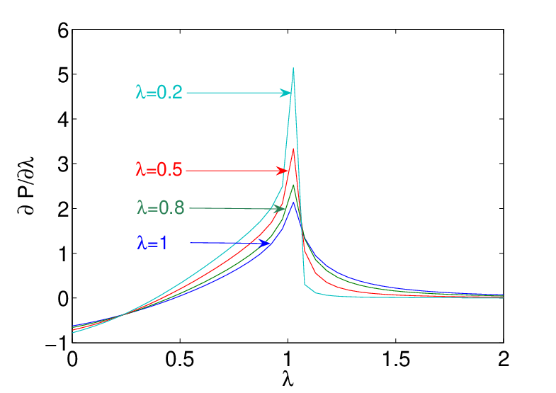
Since the magnetic moment of the spin chain changes fast at the critical points of the chain, then we may expected that the LZ transition can also reflect such property of the spin chain by the expression of (7) and (8). Fig. 2 shows the function of $\Gamma^{2}$ as well as its derivative relation with $\lambda$ and $\Delta$, we set the number of the chain $N=200$, $g=0.1J$ in the numerical illustration. It is evident that when the strength of the transverse field $\lambda\rightarrow 1$, $\Gamma^{2}$ also changes sharply. As mentioned above, in order to reveal this effect of quantum phase transitions more clearly, we may pay more attention to the derivative of $\Gamma^{2}$ by $\lambda$, which perfectly shows the quantum critical phenomenon. Just as we have expected, this property has been inherited very well by the LZ transition probability $P_{\uparrow\rightarrow\downarrow}(\infty)$ and its derivative, as Fig. 3 shows, where we have set $v=50{J^{2}/\hbar}$ in the calculation. It is in evidence that the critical point is reflected perfectly well in the derivative of LZ transition, which is consist with the above analysis.

Different values of $\Delta$ also affect the property of LZ transition probability. From Eq. (8) and Fig. 3, we may find that when $\Delta>0$, the transition probability declines first, and then reveals again, however, the sharply changed location is not influenced, which can also give us a good reflection of quantum phase transitions. When $\Delta$ is large enough, the transition probability will not reveal again in the case of $\lambda>1$.

Now we consider the case where the XY spin chain acts as the environment. Straightforward calculation shows that to get the result in this situation, we need to replace $-J\sum_{j=-M}^{M}(\frac{1+\gamma}{2}\sigma^{z}_{j}\sigma^{z}_{j+1}+\frac{1-\gamma}{2}\sigma^{y}_{j}\sigma_{j+1}^{y}+\lambda\sigma^{x}_{j})$ with $-J\sum_{j=-M}^{M}(\sigma^{z}_{j}\sigma^{z}_{j+1}+\lambda\sigma^{x}_{j})$ in Eq. (1). Here $\gamma$ measures the anisotropy in XY spin-chain. The XY Hamiltonian will turn into the transverse Ising chain for $\gamma=1$, and the XX chain in transverse field for $\gamma=0$.

By the same procedure, we can obtain the LZ transition probability in this case, the equations are nothing but changing the definition of $\theta_{k}$ and $\xi_{k}$ in the above discussions, i.e., $\cos\theta_{k}=\varepsilon_{k}/{\xi_{k}}$, in which $\varepsilon_{k}=2J(\lambda-\cos\frac{2\pi k}{N})$ and $\xi_{k}$ are now defined as $\xi_{k}=2J\sqrt{[\cos\frac{2\pi k}{N}-\lambda]^{2}+\gamma^{2}\sin^{2}\frac{2\pi k}{N}}$.

Following the same calculation, we then obtain the same expression as (7) and (8). Fig. 4 shows the relation between LZ transition probability $P$ and the anisotropy parameter, as well as its derivative $\partial P/{\partial\lambda}$. We set $N=200$, $g=0.1J$, $\Delta=5J$, $v=50{J^{2}/\hbar}$, in the numerical calculation. It shows that when $\gamma$ changes from $1$ to $0$, the critical behavior is reflected quite well in the LZ transition, and the critical line $\lambda=1$ is clearly reflected in the derivative of the LZ transition probability. We may deduce that the distinctive feature of the XX chain environment is a sharp discontinuity in the derivative $\partial P/{\partial\lambda}$ at $\lambda=1$, this is reflected more clearly from the panel in Fig. 4. This result confirm our above prediction that the LZ transition can reflect the critical points of the environment.

In summary, we have studied the Landau-Zener transitions in two-state systems coupling to the Ising spin chain and XY spin chain in transverse fields. We have calculated the exact expressions of the LZ transition probabilities of the two-state systems and analyzed the relation between their properties and the occurrence of the quantum phase transitions in the chain. The results show that the LZ transition are determined by the spin chains’ magnetic moments and their variance. As the magnetic moments of the chains contain the information of quantum phase transitions, the LZ transitions may act as the witnesses of quantum phase transitions in the chains. Our results suggest a rather intriguing relationship between LZ transitions and the environments’ properties, and therefore the results may provide a new way to study the phenomenon of quantum phase transition as well as Landau-Zener transition.