Lifetime Improvement of Wireless Sensor Networks by Collaborative Beamforming and Cooperative TransmissionThanks: This research was supported by the National Science Foundation under Grants ANI-03-38807 and CCR-02-05214.

Zhu Han Affiliation: Department of Electrical and Computer Engineering, Boise State University, Idaho, USA H. Vincent Poor Affiliation: School of Engineering and Applied Science, Princeton University, New Jersey, USA.

Abstract

Extending network lifetime of battery-operated devices is a key design issue that allows uninterrupted information exchange among distributive nodes in wireless sensor networks. Collaborative beamforming (CB) and cooperative transmission (CT) have recently emerged as new communication techniques that enable and leverage effective resource sharing among collaborative/cooperative nodes. In this paper, we seek to maximize the lifetime of sensor networks by using the new idea that closely located nodes can use CB/CT to reduce the load or even avoid packet forwarding requests to nodes that have critical battery life. First, we study the effectiveness of CB/CT to improve the signal strength at a faraway destination using energy in nearby nodes. Then, a 2D disk case is analyzed to assess the resulting performance improvement. For general networks, if information-generation rates are fixed, the new routing problem is formulated as a linear programming problem; otherwise, the cost for routing is dynamically adjusted according to the amount of energy remaining and the effectiveness of CB/CT. From the analysis and simulation results, it is seen that the proposed schemes can improve the lifetime by about 90% in the 2D disk network and by about 10% in the general networks, compared to existing schemes.

I Introduction

In wireless sensor networks [1], extending the lifetime of battery-operated devices is considered a key design issue that increases the capability of uninterrupted information exchange and alleviates the burden of replenishing batteries. In [2], a data routing algorithm has been proposed with an aim to maximize the minimum lifetime over all nodes in wireless sensor networks. A survey of energy constraints for sensor networks has been studied in [3]. In [4], the network lifetime has been maximized by employing the accumulative broadcast strategy. The work in [5] has considered provisioning additional energy in the existing nodes and deploying relays to extend the lifetime.

Recently, collaborative beamforming (CB) [6] and cooperative transmission (CT) [7][8] have been proposed communication techniques that fully utilize spatial diversity and multiuser diversity. While most existing work in this area concentrates on improving the performances at the physical layer, CB and CT also have impact on the design of higher layer protocols. In this paper, we investigate new routing protocols to improve the lifetime of wireless sensor networks using these two techniques.

First, we study the fact that CB/CT can effectively increase the signal strength at a destination node, which in turn can increase the transmission range. We obtain a closed-form analysis of the effectiveness of CT similar to that given for CB in [6]. Then, we formulate the problem as a maximization of the network lifetime, defined until the time of the first node failure. The new idea is that closely located nodes can use CB/CT to reduce the loads or even avoid packet forwarding requests to nodes with critical battery lives. From the analysis of a 2D disk case using CB/CT, we investigate how battery-depleting nodes close to the sink can be bypassed. Then we propose algorithms for a general network situation. If the information-generation rates are fixed, we can formulate the problem as a linear programming problem. Otherwise, we propose a heuristic algorithm to dynamically update costs in the routing table according to the remaining energy and effectiveness of collaboration. From the analysis and simulation results, the proposed new routing schemes can improve the lifetime by about 90% in the 2D disk network compared to the pure packet forwarding scheme, and by about 10% in general networks, compared to the schemes in [2].

This paper is organized as follows: In Section II, the system model is given, and the abilities of CB/CT to enhance the destination signal strength are studied. In Section III, we formulate the lifetime maximization problem, analyze a 2D disk case, and propose algorithms for general network situations. Simulation results are given in Section IV and conclusions are drawn in Section V.

II System Model and Effectiveness of CB/CT

We assume that a group of sensors is uniformly distributed with a density of $\rho$ . Each node is equipped with a single ideal isotropic antenna. There is no power control for each node, i.e., the node transmits with power either $P$ or $0$ . There is no reflection or scattering of the signal. Thus, there is no multipath fading or shadowing. The nodes are sufficiently separated that any mutual coupling effects among the antennas of different nodes are negligible.

For traditional direct transmission, a node tries to reach another node at a distance of $A$ . The signal to noise ratio (SNR) is given by

\Gamma=\frac{PC_{0}A^{-\alpha}|h|^{2}}{\sigma^{2}},\vskip-2.84526pt

(1)

where $C_{0}$ is a constant that incorporates effects such as antenna gains, $\alpha$ is the propagation loss factor, $h$ is the channel gain, and $\sigma^{2}$ is the thermal noise level. We define the energy cost of such a transmission for each packet to be one unit.

In Figure 1, we show the system model with CB/CT. In traditional sensor networks, the only choice a node has is to forward its information toward the sink. This will deplete the energy of the nodes near the sink, since they have to transmit many other nodes’ packets. To overcome this problem, in this paper, we propose another choice for a node consisting of forming CB/CT with the nearby nodes so as to transmit further towards the sink. By doing this, we can balance the energy usage of the nodes having different locations and different remaining energy. In the rest of this section, we study how effectively CB and CT can improve the link quality.

II-A Effectiveness of Collaborative Beamforming

Suppose there are a total of $N$ users for collaborative beamforming within a disk of radius $R$ . We have

N=\lfloor\rho\pi R^{2}\rfloor.\vskip-2.84526pt

(2)

Each node has polar coordinate $(r_{k},\psi_{k})$ to the disk center. The distance from the center to the beamforming destination is $A$ . The Euclidean distance between the $k^{th}$ node and the beamforming destination can be written as:

d_{k}=\sqrt{A^{2}+r_{k}^{2}-2r_{k}A\cos(\phi-\psi_{k})},

(3)

where $\phi$ is azimuth direction and is assumed to be a constant. By using loop control or the Global Positioning System, the initial phase of node $k$ can be set to

\psi_{k}=-\frac{2\pi}{\lambda}d_{k}(\phi),\vskip-2.84526pt

(4)

where $\lambda$ is the wavelength of the radio frequency carrier.

Define $\textbf{z}=[z_{1}\dots z_{N}]^{T}$ with

z_{k}=\frac{r_{k}}{R}\sin(\psi_{k}-\phi/2).

(5)

The array factor of CB can be written as

F(\phi|\textbf{z})=\frac{1}{N}\sum_{k=1}^{N}e^{-j4\pi R\sin(\frac{\phi}{2})z_{k}/\lambda}.\vskip-2.84526pt

(6)

The far-field beam pattern can be defined as:

	$\displaystyle P(\phi\|\textbf{z})$	$\displaystyle=$	$\displaystyle\|F(\phi\|\textbf{z})\|^{2}$		(7)
		$\displaystyle=$	$\displaystyle\frac{1}{N}+\frac{1}{N^{2}}\sum_{k=1}^{N}e^{-ja(\phi)z_{k}}\sum_{l\neq k}e^{ja(\phi)z_{l}},\vskip-2.84526pt$		(7)

where

a(\phi)=\frac{4\pi R\sin\frac{\phi}{2}}{\lambda}.

(8)

Define the directional gain $D_{av}^{CB}$ as the ratio of radiated concentrated energy in the desired direction over that of a single isotropic antenna. From Theorem 1 in [6], for large $\frac{R}{\lambda}$ and $N$ , the following lower bound for far-field beamforming is tightly held:

\frac{D_{av}^{CB}}{N}\geq\frac{1}{1+\mu\frac{N\lambda}{R}},

(9)

where $\mu\approx 0.09332$ .

Considering this directional gain, we can improve the direct transmission by a factor of $D_{av}^{CB}$ . Notice that this transmission distance gain for one transmission is obtained at the expense of consuming a total power of $N$ units from the nearby nodes.

II-B Effectiveness of Cooperative Transmission

Similar to the CB case, we assume $N$ users are uniformly distributed over a radius of $R$ . The probability density function of the users’ radial coordinate $r$ is given by

q(r)=\frac{2r}{NR^{2}},\ \ 0\leq r\leq R,

(10)

and the users’ angular coordinate $\psi$ is uniformly distributed between $[0,2\pi)$ .

Suppose at the first stage, node $1$ transmits to the next hop or sink. Then in the following stages, node $2$ to node $N$ relay the node $1$ ’s information if they decode it correctly. The received signals at node $2$ to node $k$ at stage 1 can be expressed as:

z_{k}=\sqrt{Pr_{k}^{-\alpha}}h_{k}^{r}x+n_{k}^{r},\ k=2,\dots N,

(11)

and the received signals at the destination in the following stages are

y_{k}=\sqrt{Pd_{k}^{-\alpha}}h_{k}x+n_{k}.

(12)

Here $P$ is the transmitted power, $h_{k}^{r}$ and $h_{k}$ are the channel gains of source-relay and relay-destination, which are modeled as independent zero mean circularly symmetric complex Gaussian random variables with unit variance, $x$ is the transmitted data having unit power, and $n_{k}$ and $n_{k}^{r}$ are independent thermal noises with noise variance $\sigma^{2}$ .

Theorem 1

Define $D_{av}^{CT}$ to be the energy enhancement at the destination node due to CB. Under the far-field condition and the assumption that channel links between source and relays are sufficiently good, we have the following approximation:

\frac{D_{av}^{CT}}{N}\approx\frac{1+(N-1)\ _{2}F_{1}\left(\frac{2}{\alpha},-L;\frac{\alpha+2}{\alpha};\frac{\sigma^{2}R^{\alpha}}{4P}\right)}{N},

(13)

where $L$ is the frame length and ${}_{2}F_{1}$ is the Hypergeometric function

{}_{2}F_{1}(a,b;c;z)=\sum_{n=0}^{\infty}\frac{(a)_{n}(b)_{n}}{(c)_{n}}\frac{z^{n}}{n!},

(14)

where $(a)_{n}=a(a+1)\cdots(a+n-1)$ is the Pochhammer symbol.

Proof:

The SNR received by the $k^{th}$ user at stage one can be written as

\Gamma_{k}=\frac{PC_{0}r_{k}^{-\alpha}|h_{k}^{r}|^{2}}{\sigma^{2}},

(15)

where $|h_{k}^{r}|^{2}$ is the magnitude square of the channel fade and follows an exponential distribution with unit mean.

Without loss of generality, we suppose that BPSK modulation is used and $C_{0}=1$ . The probability of successful transmission of the packet with length $L$ is given by:

P_{r}^{k}(r)=\left(\frac{1}{2}+\frac{1}{2}\sqrt{\frac{P}{P+\sigma^{2}r^{\alpha}_{k}}}\right)^{L}.

(16)

For fixed $(r_{k},\psi_{k})$ , the average energy that arrives at the destination can be written as:

D^{CT}=\sum_{k=1}^{N}Pd_{k}^{-\alpha}P_{r}^{k}.

(17)

Since for node $1$ , $r_{1}=0$ . We can write the average energy gain in the following generalized form:

D^{CT}_{av}=\sum_{k=1}^{N}\int_{0}^{R}\int_{0}^{2\pi}\frac{A^{\alpha}}{2\pi}d_{k}^{-\alpha}P_{r}^{k}(r_{k})q(r_{k})dr_{k}d\psi_{k}.

(18)

Since each user is independent of the others, we omit the notation $k$ and can rewrite (18) as:

	$\displaystyle D^{CT}_{av}=1+(N-1)$		(19)
	$\displaystyle\int_{0}^{2\pi}\int_{0}^{R}\frac{2r}{A^{-\alpha}R^{2}}(A^{2}+r^{2}-2rA\cos\psi)^{-\frac{\alpha}{2}}P_{r}(r)drd\psi.$

With the far field assumption, we have

\int_{0}^{2\pi}(A^{2}+r^{2}-2rA\cos\psi)^{-\frac{\alpha}{2}}d\psi\approx A^{-\alpha}.

(20)

The average energy gain is approximated by

D^{CT}_{av}\approx 1+(N-1)\frac{2}{R^{2}}\int_{0}^{R}rP_{r}(r)dr.

(21)

With the assumption of sufficiently good channels between sources and relays, we have the following approximation of (16):

P_{r}(r)\approx(1-\frac{\sigma^{2}r^{\alpha}}{4P})^{L}.

(22)

Since

\int_{0}^{R}r(1-\frac{\sigma^{2}r^{\alpha}}{4P})^{L}dr=\frac{1}{2}R^{2}\ _{2}F_{1}\left(\frac{2}{\alpha},-L;\frac{\alpha+2}{\alpha};\frac{\sigma^{2}R^{\alpha}}{4P}\right),

(23)

we can obtain (13). ∎

In Figure 2, we compare the numerical and analytical results of $D_{av}$ for different radii $R$ . Here $A=1000$ m, $P=10$ dbm, $\sigma^{2}=-70$ dbm, $\alpha=4$ , $L=100$ and $N=10$ . We can see that the numerical result fits the analysis very well, which suggests that the approximation in (13) is a good one.

III CB/CT Lifetime Maximization

In this section, we first define the lifetime of sensor networks and formulate the corresponding optimization problem. Then, by using a 2D disk case, we demonstrate analytically the effectiveness of lifetime saving using CB/CT. Finally, two algorithms are proposed for general network configurations.

III-A Problem Formulation

In Figure 3, we show the routing model with CB/CT. A wireless sensor network can be modeled as a directed graph $G(M,\mathbb{A})$ , where $M$ is the set of all nodes and $\mathbb{A}$ is the set of all links $(i,j),i,j\in M$ . Here the link can be either a direct transmission link or a link with CB/CT. Let $S_{i}$ be the set of nodes that the $i^{th}$ node can reach by direct transmission. Denote by $C_{i}^{m}$ the set of nodes that node $i$ needs to apply CB/CT with in order to reach node $m$ . In the example in Figure 3, $C_{i}^{m}=\{l\}$ and $C_{i}^{k}=\{\}$ . A set of origin nodes $O$ where information is generated at node $i$ with rate $Q_{i}$ can be written as:

O=\{i|Q_{i}>0,\ i\in M\}.

(24)

A set of destination nodes is defined as $D$ where

D=\{i|Q_{i}<0,\ i\in M\}.

(25)

Define $\textbf{q}=\{q_{ij}\}$ to represent the routing and the transmission rate. There are many types of definitions for lifetime of sensor networks. The most common ones are the first node failure, the average lifetime, and $\alpha$ lifetime. In this paper, we use the lifetime until first node failure as an example. Other types of lifetime can be examined in a similar way. Suppose node $i$ has remaining energy of $E_{i}$ . The lifetime for each node can be written as:

T_{i}(\textbf{q})=\frac{E_{i}}{\sum_{j\in S_{i}}q_{ij}+\sum_{i\in C_{j}^{m},\forall j,m}q_{jm}},\vskip-2.84526pt

(26)

where the first term in the denominator is for direct transmission and the second term in the denominator is for CB/CT. Notice that $C_{j}^{m}$ is not a function of q. We formulate the problem as

\max_{\textbf{q}}\ \min T_{i}

(27)

\mbox{s.t. }\left\{\begin{array}[]{l}q_{ij}\geq 0,\forall i,j\\ \sum_{j,i\in S_{j}}q_{ij}+Q_{i}=\sum_{k\in S_{i}}q_{ik},\\ \end{array}\right.

where the second constraint is for flow conservation.

III-B 2D Disk Case Analysis

In this subsection, we study a 2D disk case network. Users with the same remaining energy are uniformly located within a circle of radius $B_{0}$ . One sink is located at the center location $(0,0)$ . Each node has a unit amount of information to transmit. Here we assume the user density is large enough, so that each node can find enough nearby nodes to form CB/CT to reach the faraway node.

For traditional packet forwarding without CB/CT, the number of packets needing transmission for each node at the distance $B$ to the sink is given by

N_{pf}(B)=\sum_{n=0}^{\lfloor\frac{B_{0}-B}{A_{0}}\rfloor}\left(1+\frac{nA_{0}}{B}\right).\vskip-2.84526pt

(28)

where $A_{0}$ is the maximal distance over which a minimal link quality $\gamma_{0}$ can be maintained, i.e. $\Gamma(A_{0})=\gamma_{0}$ .

If all nodes use their neighbor nodes to communicate with the sink directly, we call this scheme pure CB/CT. To achieve the range of $B$ , we need $N_{CB/CT}(B)$ for CB/CT, i.e.,

D_{av}\left(\sqrt{\frac{N_{CB/CT}(B)}{\rho\pi}}\right)=\left(\max(\frac{B}{A_{0}},1)\right)^{\alpha}.\vskip-2.84526pt

(29)

For collaborative beamforming, we can calculate

N_{CB}(B)\geq\frac{1}{2}\left(c_{0}(2+c_{0}c_{1}^{2})+c_{0}^{1.5}c_{1}\sqrt{4+c_{0}c_{1}^{2}}\right)\vskip-2.84526pt

(30)

where $c_{0}=(\max(\frac{B}{A_{0}},1))^{\alpha}$ and $c_{1}=\mu\lambda\sqrt{\rho\pi}$ . For cooperative transmission, numerical results need to be used to obtain the inverse of ${}_{2}F_{1}$ in Theorem 1. Notice that if the node density is large enough, then $D_{av}/N\longrightarrow 1$ .

In Figure 4, we show the average transmission per node vs. the disk size $B_{0}$ . We can see that for traditional packet forwarding, the node closest to the sink has the most transmissions per node, i.e., it has the lowest lifetime if the initial energy is the same for all nodes. On the other hand, for the pure CB/CT scheme, more nodes need to transmit to reach the sink directly when $B_{0}$ is larger. The transmission is less efficient than packet forwarding, since the propagation loss factor $\alpha$ is larger than $1$ . The above facts motivate the joint optimization case where nodes transmit packets with different probabilities over traditional packet forwarding and CB/CT.

For traditional packet forwarding, nodes near the sink have lower lifetimes. If the faraway nodes can form CB/CT to transmit directly to the sink and bypass these life depleting nodes, the overall network lifetime can be improved. Notice that in this special case, if the faraway nodes form CB/CT to transmit to nodes other than the sink, the lifetime will not be improved. For each node with distance $B$ to the sink, and supposing the probability of using CB/CT is $P_{r}(B)$ , we have

	$\displaystyle N_{joint}(B)=(1-P_{r}(B)+N_{CB/CT}(B)P_{r}(B))$
	$\displaystyle\sum_{n=0}^{\lfloor\frac{B_{0}-B}{A_{0}}\rfloor}\left(1+\frac{nA_{0}}{B}\right)\Pi_{j=1}^{n}(1-P_{r}(B+jA_{0})),\vskip-2.84526pt$		(31)

where the first term on the right-hand side (RHS) is the necessary energy for transmitting one packet, and the second term is the number of packets for transmission. The goal is to adjust $P_{r}(B)$ such that the lifetime is maximized, i.e.,

\min_{1\geq P_{r}(B)\geq 0}\max N_{joint}(B).\vskip-2.84526pt

(32)

Notice that $N_{CB/CT}\geq 1$ , and in (III-B) the second term on the RHS depends on the probabilities of CB/CT being larger than $B$ . So we can develop an efficient bisection search method to calculate (32). We define a temperature $\kappa$ that is assumed to be equal or greater than $N_{joint}(B),\forall B$ . We can first calculate $N_{joint}(B)$ from the boundary of the network where the second term on the RHS of (III-B) is one. Then we can derive all $N_{joint}(B)$ by reducing $B$ . If $\kappa$ is too large, most information is transmitted by CB/CT, and the nodes faraway from the sink waste too much power for CB/CT; on the other hand, if $\kappa$ is too small, the nodes close to the sink must forward too many packets. A bisection search method can find the optimal values of $\kappa$ and $N_{joint}(B)$ .

TABLE I: Lifetime Saving vs. Disk Size

$R_{0}$	2	4	6	8	10
$\max N_{joint}(B)$	2.82	10.25	23.4	42.5	64.5
Saving %	94.56	93.33	90.86	88.13	85.98

In Figure 4, we show the joint optimization case where the node density is sufficiently large. We can see that to reduce the packet forwarding burdens of the nodes near the sink, the faraway nodes form CB/CT to transmit to the sink directly. This will increase the number of transmissions per node for them, but reduce the transmissions per node for the nodes near the sink. In Table I, we show the maximal $N_{joint}(B)$ and the lifetime saving over the traditional packet forwarding. We can see that the power saving is around 90%.

III-C General Case Algorithms

In this section, we first consider the case in which the information generation rates are fixed for all sensors, and develop a linear programming method to calculate the routing table. Here to simplify the calculation of set $C_{j}^{m}$ , we assume its size equals one. Obviously, this is suboptimal for (27). Then we select the nearest neighbor for CB/CT. $C_{j}^{m}=1$ , if node $j$ ’s nearest neighbor can help node $j$ to reach node $m$ . Define $\hat{q}_{ij}=Tq_{ij}$ . The problem can be written as a linear programming problem:

\max\ T

(33)

\mbox{s.t. }\left\{\begin{array}[]{l}\hat{q}_{ij}\geq 0,\forall i,j;\\ (\sum_{j\in S_{i}}\hat{q}_{ij}+\sum_{i\in C_{j}^{m},\forall j,m}\hat{q}_{jm})\leq E_{i},\ \forall i;\\ \sum_{j,i\in S_{j}}\hat{q}_{ji}+TQ_{i}=\sum_{k\in S_{i}}\hat{q}_{ik},\forall i\in M-D,\end{array}\right.\vskip-2.84526pt

where the second constraint is the energy constraint and the third constraint is for flow conservation.

Next, if the information rate is random, each sensor dynamically updates its cost according to its remaining energy and with consideration of CB/CT. Some heuristic algorithms can be proposed to update the link cost dynamically. Here the initial energy is $E_{i}$ . Define the current remaining energy as $\underline{E}_{i}$ . We define the cost for node $i$ to communicate with node $j$ as

\mbox{cost}_{ij}=\left(\frac{E_{i}}{\underline{E}_{i}}\right)^{\beta_{1}}+\sum_{l\in C_{i}^{j}}\left(\frac{E_{l}}{\underline{E}_{l}}\right)^{\beta_{2}},

(34)

where $\beta_{1}$ and $\beta_{2}$ are positive constants. Their values determine how the packets are allocated between the energy sufficient and energy depleting nodes, and between the direct transmission and CB/CT. Notice that (34) can be viewed as an inverse barrier function for $\underline{E}_{i}\geq 0$ .

IV Simulation Results

We assume nodes and one sink are randomly located within a square of size $\mathbb{L}\times\mathbb{L}$ . Each node has power of 10dbm and the noise level is -70dbm. The propagation loss factor is $4$ . The minimal link SNR is 10dB. The initial energy of all users is assumed to be unit and information rates for all users are 1.

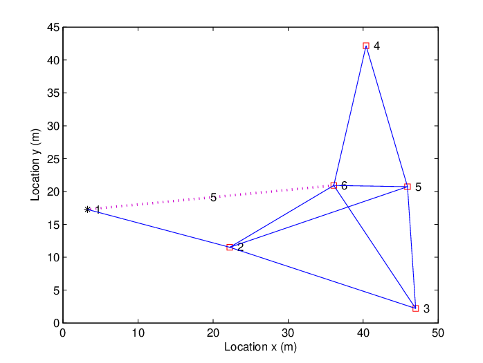
In Figure 5, we show a snapshot of a network of $5$ sensor nodes and a sink with $\mathbb{L}=50$ m. Here node $1$ is the sink. The solid lines are the links for the direct transmission, and the dotted line from node $6$ to the sink is the CB/CT link with the help of node $5$ . For traditional direct packet forwarding scheme, the best flow is

\hat{q}_{ij}=\left[\begin{array}[]{cccccc}0&0&0&0&0&0\\ 1&0&0&0&0&0\\ 0&0.2&0&0&0&0\\ 0&0&0&0&0.1&0.1\\ 0&0.3&0&0&0&0\\ 0&0.3&0&0&0&0\\ \end{array}\right]\vskip-2.84526pt

(35)

with the resulting energy consumed for all nodes given by $[0,1.0,0.2,0.2,0.3,0.3]$ . Because node $2$ is the only node that can communicate with the sink, the best lifetime of this routing is $0.2$ before node $2$ runs out of energy.

With CB/CT, the best flow is

\hat{q}_{ij}=\left[\begin{array}[]{cccccc}0&0&0&0&0&0\\ 1&0&0&0&0&0\\ 0&0.321&0&0&0&0.012\\ 0&0&0&0&0&0.333\\ 0&0.23&0&0&0&0.103\\ 0.667&0.115&0&0&0&0\\ \end{array}\right]

(36)

with the energy consumed for all nodes given by $[0,1.000,0.333,0.333,1.0000,0.782]$ . Here some flow can be sent to the sink via node $6$ . Because of CB/CT, node $5$ has to consume its power. The lifetime becomes $0.333$ which is 67% improvement over direct packet forwarding.

In Figure 6, we compare the performance of three algorithms, the shortest path, the algorithm in [2], and the proposed CB/CT algorithm. Here $\mathbb{L}=100$ m. As the number of users increases, the performance of the shortest path algorithm decreases. This is because more users will need packet forwarding by the nodes near the sink. Consequently, they die more quickly. Compared with the algorithm in [2], the proposed schemes have about 10% performance improvement. This is because of the alternative routes to the sink that can be found by CB/CT.

V Conclusions

In this paper, we have studied the impact of CB/CT on the design of higher level routing protocols. Specifically, using CB/CT, we have proposed a new idea based on bypassing energy depleting nodes that might otherwise forward packets to the sink, in order to improve the lifetime of wireless sensor networks. From the analytical and simulation results, we have seen that the proposed protocols can increase lifetime by about 90% in a 2D disk case and about 10% in general network situations, compared with existing techniques.

References

[1] I. F. Akyildiz, W. Su, Y. Sankarasubramaniam, and E. Cayirci, “A survey on sensor networks,” IEEE Communications Magazine., Vol. 40, Issue: 8 , pp. 102-114, Aug. 2002.
[2] J. H. Chang and L. Tassiulas, “Energy conserving routing in wireless ad-hoc networks,” in Proceedings of INFOCOM 2000, Tel-Aviv, Israel, March 2000, pp. 22-31.
[3] A. Ephremides, “Energy concerns in wireless networks,” IEEE Wireless Communications, vol. 9, no. 4, pp. 48-59, Aug. 2002.
[4] I. Maric and R. D. Yates, “Cooperative broadcast for maximum network lifetime,” Proc. Conf. on Inform. Sciences and Systems, The Johns Hopkins University, Baltimore, MD, vol. 1, pp. 591-596, 2004.
[5] Y. T. Hou, Y. Shi, H. D. Sherali, and S. F. Midkiff, “On energy provisioning and relay node placement for wireless sensor networks,” IEEE Trans. Commun., vol 4, pp. 2579-2590, Sept. 2005.
[6] H. Ochiai, P. Mitran, H. V. Poor, and V. Tarokh, “Collaborative beamforming for distributed wireless ad hoc sensor networks”, IEEE Trans. Signal Processing, vol. 53, no. 11, pp. 4110-4124, Nov. 2005.
[7] A. Sendonaris, E. Erkip, and B. Aazhang, “User cooperation diversity, Part I: System description,” IEEE Trans. Commun., vol. 51, pp.1927-1938, Nov. 2003.
[8] J. N. Laneman, D. N. C. Tse, and G. W. Wornell, “Cooperative diversity in wireless networks: Efficient protocols and outage behavior,” IEEE Trans. Inform. Theory, vol. 50, no. 12, pp. 3062-3080, Dec. 2004.