Exact fuzzy sphere thermodynamics in matrix quantum mechanics Preprint: KEK-TH-1145
Abstract:
We study thermodynamical properties of a fuzzy sphere in matrix quantum mechanics of the BFSS type including the Chern-Simons term. Various quantities are calculated to all orders in perturbation theory exploiting the one-loop saturation of the effective action in the large- limit. The fuzzy sphere becomes unstable at sufficiently strong coupling, and the critical point is obtained explicitly as a function of the temperature. The whole phase diagram is investigated by Monte Carlo simulation. Above the critical point, we obtain perfect agreement with the all order results. In the region below the critical point, which is not accessible by perturbation theory, we observe the Hagedorn transition. In the high temperature limit our model is equivalent to a totally reduced model, and the relationship to previously known results is clarified.
Keywords:
Non-Commutative Geometry, Matrix Models, Thermal Field Theory1 Introduction
Fuzzy sphere [1], which is a simple compact noncommutative manifolds, has been discussed extensively in the literature. One of the motivations comes from the general expectation that noncommutative geometry provides a crucial link to string theory and quantum gravity. Indeed Yang-Mills theories on noncommutative geometry appear in a certain low energy limit of string theory [2]. There is also an independent observation that the space-time uncertainty relation, which is naturally realized by noncommutative geometry, can be derived from some general assumptions on the underlying theory of quantum gravity [3]. As another motivation, fuzzy manifolds may be used as a novel regularization method in quantum field theories [4].
In string theory, fuzzy spheres appear as D-branes in the presence of external fields [5]. In particular they appear as classical solutions11 1 More general classical solutions such as a rotating fuzzy sphere are discussed in refs. [6, 7, 8, 9, 10]. in the pp-wave matrix model [11], which is a generalization of the BFSS matrix theory [12] to the so-called pp-wave background [13]. Fundamental issues such as the stability of these solutions [14, 15, 10] and the spectrum of the fluctuations [14, 16, 17, 18] have been studied intensively.22 2 Similarly, fuzzy spheres appear as classical solutions in matrix string theory [19] on a type IIA plane-wave background [20]. The spectrum around the fuzzy spheres is computed in ref. [21]. This theory is used to study the matrix big bang [22].
Thermodynamical properties of the pp-wave matrix model have also been studied by various authors. In ref. [23] the free energy around the trivial vacuum, which corresponds to a transverse M5-brane [24] at zero temperature33 3 A fuzzy five-sphere solution was constructed [25] in a deformed plane-wave matrix model with an interaction term due to the 6-form potential., was evaluated at the one-loop level, and the Hagedorn transition was studied in detail. (See refs. [26, 27] for a two-loop extension and ref. [28] for a review on this subject.) This calculation have been extended to more general vacua in refs. [29, 30, 31]. In all these works, however, a mass parameter, which parametrizes the deviation from the flat background, is assumed to be large so that higher loop effects can be neglected.
In this paper we show that in fact it is possible to study the fuzzy sphere thermodynamics to all orders in perturbation theory. While the method can be applied to more general models including the pp-wave matrix model, here we demonstrate it in a simple model, which can be obtained by dimensionally reducing a 4d U() gauge theory to 1d. The model has been used recently to compute the mass gap in the theory of bosonic membranes [32]. The action contains the 3d Chern-Simons term representing the coupling to a background flux [5], which enables fuzzy spheres to appear as classical solutions. When the Chern-Simons coupling is switched off, it reduces to the “4d bosonic BFSS matrix theory” [33]. Studying matrix quantum mechanics at finite temperature44 4 More generally, large- gauge theory at finite temperature has been an active field of research [34, 35, 36, 37, 38] partly motivated from the gauge/gravity correspondence. is itself an interesting subject [39, 40, 41, 35], in particular, because of its relation to the black hole physics [42, 43, 44].
The method for the all order calculation has been developed in totally reduced models [45, 46], which are motivated in the context of the type IIB matrix model [47]. The key observation is that, in the large- limit, the effective action is saturated at one loop in the bosonic case [46], and at two loop in the supersymmetric case [45]. Through the Legendre transformation, one can obtain the free energy and various observables to all orders. (We emphasize that this is different from a typical situation in supersymmetric field theories, in which higher loop corrections simply vanish due to cancellation.) In the bosonic case, it has been confirmed that the all order results are in perfect agreement with the Monte Carlo results [48] obtained in the fuzzy sphere phase. These works have also been extended to four-dimensional fuzzy manifolds [49, 50].
Similarly to the results in ref. [48], we find in the present finite-temperature system that a single fuzzy sphere becomes unstable at some critical , the coefficient of the Chern-Simons term. This phenomenon occurs at any temperature, and we obtain explicitly the critical as a function of the temperature. We also perform Monte Carlo simulation and confirm that the all order results for various observables agree very well with the Monte Carlo results above the critical . In the region below the critical , which is not accessible by perturbation theory, we observe the Hagedorn transition at some critical temperature. At high temperature our model is equivalent to a totally reduced model, which is analogous to the model studied in ref. [48]. We clarify the relationship to the results obtained there.
The rest of this paper is organized as follows. In section 2 we define our model and discuss its classical solutions. In section 3 we show how one can perform the all order calculation in perturbation theory. In section 4 we compare the all order results with the Monte Carlo results. In section 5 we study the region in the phase diagram below the critical , and show that the Hagedorn transition takes place. In section 6 we discuss the high temperature limit of the model. Section 7 is devoted to a summary and discussions.
2 The model and its classical solutions
The model we study in this paper is defined by the action55 5 We could have replaced the overall factor of in the action (1) by , where represents the Yang-Mills coupling constant. Our choice would then correspond to setting the ’t Hooft coupling to unity. We do not lose any generality, however, since the model for arbitrary can be readily obtained by rescaling , , .
| (1) |
where represents the covariant derivative The dynamical variables and are Hermitian matrices, which can be regarded as the gauge field and three adjoint scalars, respectively, in a 1d gauge theory with the U() gauge symmetry
| (2) |
The Euclidean time in (1) has a finite extent , which is related to the temperature through , and all the fields obey periodic boundary conditions. The cubic term represents the Chern-Simons term, which is crucial for fuzzy spheres to become classical solutions. The case corresponds to the “4d bosonic BFSS model” studied in refs. [33].
The classical equations of motion can be obtained from the action (1) as
| (3) | |||||
| (4) |
There are two types of static solutions. The first type is given by configurations with and being static and diagonal. The action vanishes identically for such configurations, and therefore all the diagonal elements are moduli parameters. The second type of solutions can be represented as
| (5) |
where represents the -dimensional irreducible representation of the algebra and the parameters and satisfy The Hermitian matrices are arbitrary, and they represent the moduli parameters. For this type of classical solutions, the action is evaluated as
| (6) |
which becomes minimum for , , . In this case the solution simply becomes
| (7) |
which represents a single fuzzy sphere with the radius , since it satisfies (“Fuzzy” because of the non-trivial commutation relation among .)
3 Perturbative calculation around the fuzzy sphere
3.1 Exact effective action and the critical point
In this subsection we calculate the one-loop effective action around a configuration , which reduces to the single fuzzy sphere solution for . It is known that the effective action around a fuzzy sphere configuration is “one-loop exact” in the sense that higher order corrections vanish in the large- limit [46, 49, 50]. From the effective action, we can obtain the critical coupling , below which the fuzzy sphere becomes unstable due to both quantum and thermal fluctuations.
Let us first expand and around the rescaled single fuzzy sphere as
| (8) |
where the fields and represent the fluctuation. Since the original action (1) has a gauge symmetry (2), we fix the gauge by adding the gauge-fixing term and the ghost term as
| (9) | |||||
| (10) | |||||
| (11) |
Plugging (8) into eq. (9), we obtain , where66 6 We have omitted a term in eq. (13), which does not contribute to the effective action at one loop.
| (12) | |||||
| (13) | |||||
| (14) | |||||
while the linear term and the quartic term will not be needed in the following calculation. In eq. (13), we have introduced the adjoint operation on an matrix . Following the usual procedure, the effective action can be calculated as , where the classical term is nothing but , and the one-loop term is given as
| (15) |
by performing the Gaussian integration over the fluctuation fields with the quadratic terms (13). When taking the determinant in eq. (15), we omit the zero mode corresponding to the constant mode proportional to the unit matrix. In order to diagonalize the operator , we introduce the matrix analog of the spherical harmonics (, ), which obeys the orthonormal relations
| (16) |
and has the following properties as a representation of the SU(2) algebra
| (17) | |||||
where . Using the formula , we obtain
| (18) |
Here we have omitted a -independent constant,77 7 This constant becomes relevant, e.g., when one compares free energy for different types of vacua [31]. which is irrelevant for the following analysis.
When we take the large- limit of the effective action, we have to scale the parameters , and in such a way that the classical term and the one-loop term become the same order. This motivates us to introduce the rescaled parameters
| (19) |
The sum over in eq. (18) can be evaluated in the large- limit with fixed and . Thus we obtain the exact effective action as
| (20) |
The function is defined as
| (21) | |||||
where the polylogarithm function and the Riemann zeta function are defined, respectively, as and .
The local minimum of the effective action, which corresponds to the quantum fuzzy sphere, can be obtained by solving
| (22) |
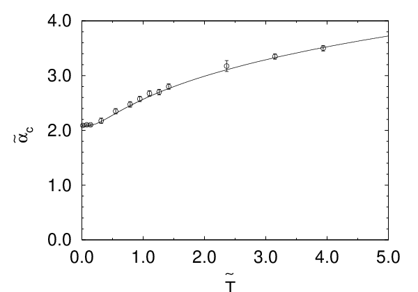
with respect to in the region . As we decrease , we find that the local minimum disappears at some critical point , which depends on . The critical point obtained in this way is plotted against in figure 2. In particular, the asymptotic behaviors of the critical point at the low and high limits are given by
| (23) |
3.2 One-loop calculation of observables
In this subsection we calculate the expectation values of the operators
| (24) |
around the single fuzzy sphere (7) at one loop. Unlike the effective action, the expectation values do have higher-loop corrections, which shall be obtained in a resummed form in the next subsection.
Let us decompose the fields into the background and fluctuations as in eq. (8), where we set in this subsection. The expectation value can be represented as
| (25) |
The first term can be easily evaluated as
| (26) |
The second term can be evaluated at one loop using the cubic terms (14) as
| (27) | |||||
where the symbol represents the expectation value using the quadratic terms (13) only. Eq. (27) can be evaluated by using the Wick theorem. The propagators can be derived from the quadratic terms (13) as
| (28) | |||||
| (29) | |||||
| (30) |
where the indices run over and is defined as
| (31) |
The symbol implies that the zero mode is omitted by excluding for . Using the formula , eq. (27) can be evaluated as
| (32) |
The sum over can be evaluated at large as in (21) for fixed and , and it turns out that (32) is given by . Since the third term of eq.(25) is suppressed at large , is obtained at one loop as
| (33) |
The expectation values of and can be calculated in a similar way, but it is much easier to obtain them by making use of the fact that these operators appear in the action (1). The expectation values can therefore be rewritten as88 8 Eq. (35) can be derived by introducing a source term in the action, and by absorbing it by rescaling the variables as , , with an appropriate . Since the integration measure and the kinetic term in the action are invariant under this transformation, the free energy for the action with the source term can be obtained by simply rescaling and .
| (34) | |||||
| (35) |
Here the free energy is defined by
| (36) |
and at one loop it can be obtained from the effective action by simply replacing by . In the large- limit with fixed and , we get
| (37) |
Plugging this into (34) and (35), we obtain
| (38) | |||||
| (39) |
3.3 All order calculation of observables
In this subsection we exploit the fact that the effective action is saturated at one loop in the large- limit, and calculate the expectation values of the operators , and to all orders in perturbation theory. The crucial point here is that the free energy and the effective action are related to each other by the Legendre transformation. Therefore, we can obtain the free energy by evaluating the effective action at its local minimum. Since the expectation values can be obtained by differentiating the free energy (for an action including an additional source term if the operator does not exist in the original action), we can obtain the all order results for the expectation values in the large- limit. This amounts to [46] keeping only the terms in the one-loop result that come from 1PI diagrams, and replacing by the solution to eq. (22), which we denote as in what follows. Since the one-loop contributions to and come only from 1PR diagrams, the corresponding all order results are readily obtained from the classical results by replacing by as
| (40) | |||||
| (41) |
Let us next consider . Since the one-loop contribution to includes both 1PI diagrams and 1PR diagrams, it is easier to obtain the all order result by using the relation (35). As explained above, the free energy is given to all orders in perturbation theory as
| (42) |
When we differentiate with respect to and , we have to take into account that depends on and . Thus we obtain
| (43) | |||||
where the coefficients and are given as
| (44) | |||||
| (45) |
4 Comparison with Monte Carlo results
In this section we compare the all order results obtained in the previous section with the results of Monte Carlo simulation taking the single fuzzy sphere (7) as the initial configuration. The lattice formulation and the algorithm used for simulating the model (1) is the same as in ref. [51]. The lattice spacing and the number of sites in the Euclidean time direction obey the relation . We have chosen these lattice parameters so that our results represent the continuum limit with sufficiently good accuracy.99 9 More precisely, the lattice parameters are chosen to satisfy both and at any temperature, where is used for figures 1 and 3 (except for the right bottom panel), and otherwise. See ref. [52] for an analysis on finite lattice spacing effects in a related model.
4.1 Boundary of the fuzzy sphere phase


Let us first investigate how the observables (24) behave as a function of . This, in particular, allows us to determine the critical , below which the single fuzzy sphere becomes unstable.
In figure 1 we plot the expectation values , , against for fixed close to . Monte Carlo results show a discontinuity at , which agrees with the result (23) at . Above the critical point, Monte Carlo results for lie on top of each other as expected from perturbation theory, and they agree very well with the all order results given by (40), (41) and (43). We have also plotted the classical results and the one-loop results for comparison. It clearly demonstrate the existence of higher-loop corrections, which are included in the all order results.
In Monte Carlo simulation we also calculate the Polyakov line
| (46) |
where the symbol represents the path-ordered exponential. Results for are shown in the right bottom panel of figure 1. We observe a gap at the same as the other observables. The properties of the Polyakov line will be discussed later in more detail.
From Monte Carlo simulations at various , we obtain the critical as a function of , which is plotted in figure 2. We observe perfect agreement with the results obtained from the one-loop effective action in the large- limit. This confirms that the effective action is indeed saturated at one loop.
We call the region above the critical line the fuzzy sphere phase, and the region below the critical line the Yang-Mills phase, following the terminology used in ref. [48]. The phase transition between the fuzzy sphere phase and the Yang-Mills phase continues to be of first order at any temperature, judging from the existence of discontinuity. In section 5 we will see that the Yang-Mills phase is further divided into two phases by the Hagedorn transition.
4.2 Temperature dependence of observables
Next we investigate the temperature dependence of observables. In figure 3 we plot the expectation values , , against for . There is a gap at , as expected from figure 2. The all order results reproduce the dependence of the observables very well below the critical . Thermal effects tend to shift the observables towards the values above the critical temperature.


In the right bottom panel of figure 3, we plot the Polyakov line as a function of . We have magnified the small region in order to see how the Polyakov line decreases as approaches 0. (Note that the scale of in this plot is an order of magnitude smaller than in other plots in figure 3.) Our results can be nicely fitted to the behavior
| (47) |
which suggests that the system is in the “deconfined phase”. The fitting parameter corresponds to the energy increase caused by a single heavy “quark”. From this figure we conclude that the center symmetry is always broken at . This statement needs some care, however. See footnote 11.
5 Hagedorn transition in the Yang-Mills phase
In this section we investigate the properties of the Yang-Mills phase. Perturbation theory is not applicable here, but Monte Carlo simulation continues to be a reliable method.

In figure 4 the Polyakov line is plotted against . We find that it changes very rapidly at the temperature , which we denote as . Above , the data are clearly nonzero, and they have little dependence on . Below , the data are consistent with decreasing as at large . Thus our data suggest that the center symmetry is spontaneously broken at . This transition can be interpreted as the Hagedorn transition [34, 23], and the critical temperature is referred to as the Hagedorn temperature in what follows. The value of is close to the result obtained in ref. [33]1010 10 Note, however, that the lattice model studied in ref. [33] is written in terms of unitary matrices instead of Hermitian matrices , and it agrees with our model only after replacing by and truncating the action at the leading order in the lattice spacing . Let us also note that an analogous model with 9 (instead of 3) Hermitian matrices has been studied by Monte Carlo simulation [35, 51] from different motivations. In that case the phase transition occurs at , which is slightly lower than the present model., where is the ’t Hooft coupling constant, which is set to unity in our analysis. (See footnote 5.)


In figure 5 we plot the observables and against at for . The results for different lie on top of each other, which implies a clear large- scaling behavior. In the confined phase , we find that the results are independent of . This can be considered as a consequence of the Eguchi-Kawai equivalence,1111 11 Let us note that the results in the fuzzy sphere phase are also consistent with Eguchi-Kawai’s statement. If we fix rather than in the large- limit, the Polyakov line vanishes identically, and all the observables have no dependence on . On the other hand, if we fix in the large- limit, the Polyakov line vanishes only at , and all the observables have non-trivial dependence on . which states the volume independence of single-trace operators in -dimensional U() gauge theory provided that the U(1)D symmetry is not spontaneously broken [53].
We have performed a similar analysis at , which is barely below the boundary of the fuzzy sphere phase. (See figure 2.) The Hagedorn temperature turned out to be as well. In the Yang-Mills phase, the Chern-Simons term takes small values as one can see from figure 1, and the observables have little dependence on . This property is found also in the totally reduced model studied in ref. [48]. Note also that the Hagedorn temperature is an O(1) quantity, which means that vanishes in the limit. In other words, if we drew the critical line corresponding to the Hagedorn transition in figure 2, it would be pushed towards the line in the large- limit. This is simply a reflection of the fact that, in the fuzzy sphere phase, we have to consider super high temperature to see non-trivial temperature dependence.
6 Fuzzy-sphere/Yang-Mills transition at high temperature
In general, field theories at high temperature are effectively described by bosonic field theories in one dimension less. This phenomenon provides a useful approach to QCD at high temperature. (See, for instance, refs. [54, 55] and references therein.) In the present model,1212 12 The high temperature limit in matrix quantum mechanics is also discussed refs. [56, 35, 57]. we do not have the subtlety related to infrared divergences unlike in ordinary field theories, since there is no infinitely extended spatial directions from the outset.
The dimensionally reduced model is obtained from the original action (1) by suppressing the dependence of the 1d fields as
| (48) | |||||
where the Greek indices , run over and we have defined
| (49) | |||||
| (50) |
The observables studied in the previous sections can be obtained at high temperature as
| (51) | |||||
| (52) | |||||
| (53) | |||||
| (54) |
The symbol represents the expectation value with respect to the dimensionally reduced model (48), where is related to through (50).
In the case, the corresponding dimensionally reduced model (48) is studied in detail at large [58]. For instance, we have
| (55) | |||||
| (56) |
Taking into account that the Greek indices run from 1 to 4 in contrast to the Roman indices, which run from 1 to 3, we obtain the asymptotic behavior of the original model with at high as
| (57) | |||||
| (58) |
Figures 4 and 5 show that our Monte Carlo results approach these results at high . (Small deviations can be nicely reproduced by the next-leading order calculation [57].)
In the fuzzy sphere phase, we can confirm the dimensional reduction analytically by using the all order calculation in perturbation theory. By taking the limit in the results for the full model, we obtain the all order results for the dimensionally reduced model, which can be obtained similarly to ref. [46]. In contrast to the situation in the Yang-Mills phase, instead of has to be large (in the large- limit) in order for the dimensional reduction to take place.


Using the dimensionally reduced model (48), let us investigate the phase transition between the fuzzy sphere phase and the Yang-Mills phase in the high temperature limit. This clarifies, in particular, the first order nature of the phase transition, and it also enables us to make explicit the connection to the known results in a totally reduced model [48]. We perform Monte Carlo simulation1313 13 We have used the same algorithm as in ref. [48]. of the dimensionally reduced model (48) using, as the initial configuration, either of the two configurations given by
| (59) |
and for both cases. In figure 6 (Left) we plot the observable appearing on the right hand side of eq. (51) against for . For comparison we also plot the all order results for the dimensionally reduced model obtained from the perturbation theory around the single fuzzy sphere in the large- limit. The Monte Carlo results depend on the initial configuration in the intermediate region of , and we observe discontinuities at
| (60) |
which we call the lower/upper critical points, respectively. (See figure 6 (Right) for a plot showing the large- behaviors.) This clearly demonstrates that the phase transition is of first order.
In a similar model [48], which can be obtained by simply omitting from (48), the critical points are obtained as and , respectively. We find that the inclusion of the fourth matrix changes the numerical coefficients, but not the powers of , in the large- behavior of the critical points.
Using the relation (50), we obtain the critical points in terms of the parameters of the full model as
| (61) |
In this terminology, the critical point shown in figure 2 is actually the lower critical point. Note that the factor in (61) is absorbed by the rescaling (19) of and , and the result agrees with the high behavior (23) obtained from the effective action.
7 Summary and discussions
We have studied thermodynamical properties of a fuzzy sphere in a BFSS-type matrix model including the Chern-Simons term. We have established the phase diagram in the -plane, and obtained, in particular, the phase boundary between the fuzzy sphere phase and the Yang-Mills phase as shown in figure 2.
In the fuzzy sphere phase, we are able to obtain all order results for various observables exploiting the one-loop saturation of the effective action in the large- limit. This technique was previously applied to various fuzzy manifolds in totally reduced models. We consider it interesting that it can be generalized to a finite temperature setup in a straightforward manner. Following refs. [49, 50] thermodynamical properties of four-dimensional fuzzy manifolds such as fuzzy and fuzzy can be studied in a similar way.
One of the interesting aspects of our results is the scaling of parameters in the large- limit. In the fuzzy sphere phase, if one fixes the original parameters and in the large- limit, one simply obtains trivial results corresponding to the classical fuzzy sphere at zero temperature. In order to keep non-trivial quantum corrections and thermal effects, one has to hold and fixed in the large- limit.
In that limit, we find that the Polyakov line vanishes smoothly as approaches . This implies that the fuzzy sphere phase is not further divided into the confined phase and the deconfined phase, unlike the Yang-Mills phase. If we take the large- limit at fixed , we are always in the confined phase. If we take the large- limit at fixed nonzero , we are always in the deconfined phase. In ref. [23] it is stated that the Hagedorn temperature for the fuzzy sphere is in an analogous model. We consider that our results provide a more precise formulation of that statement.
As an outlook, we note that fuzzy manifolds [59, 60, 61] are also studied intensively in the IIB matrix model [47] in order to investigate the dynamical generation of 4d space-time. The same issue has been addressed by various approaches [62, 63, 64, 65, 66, 67, 68, 69], and in ref. [68] the first evidence for such a phenomenon is obtained by the Gaussian expansion method. Based on the Eguchi-Kawai equivalence [53], two of the authors (N.K. and J.N.) conjectured [52] that a similar phenomenon should occur in the BFSS matrix model [12]. We therefore consider that studying the effective action for fuzzy manifolds in the BFSS matrix model would be an interesting future direction. In that case, the effective action is expected to be saturated at two loop similarly to the situation in the IIB matrix model [45].
From the view point of the gauge/gravity correspondence, the fuzzy sphere solutions in the pp-wave matrix model can be interpreted as giant gravitons. It would be interesting to look for phenomena in the dual gravity theory corresponding to the ones discussed in this paper.
Acknowledgments
We would like to thank Takehiro Azuma, Kazuyuki Furuuchi, Yoshihisa Kitazawa, Shun’ya Mizoguchi, Kentaroh Yoshida and Gordon Semenoff for valuable comments and discussions. The simulations were performed on the PC clusters at KEK.
References
- [1] J. Madore, The fuzzy sphere, Class. and Quant. Grav. 9 (1992) 69.
- [2] N. Seiberg and E. Witten, String theory and noncommutative geometry, J. High Energy Phys. 9909 (1999) 032 [hep-th/9908142].
- [3] S. Doplicher, K. Fredenhagen and J.E. Roberts, The quantum structure of spacetime at the Planck scale and quantum fields, Commun. Math. Phys. 172 (1995) 187 [hep-th/0303037].
- [4] H. Grosse, C. Klimcik and P. Presnajder, Towards finite quantum field theory in noncommutative geometry, Int. J. Theor. Phys. 35 (1996) 231 [hep-th/9505175].
- [5] R. C. Myers, Dielectric-branes, J. High Energy Phys. 9912 (1999) 022 [hep-th/9910053].
- [6] D. Bak, Supersymmetric branes in pp wave background, Phys. Rev. D 67 (2003) 045017 [hep-th/0204033].
- [7] S. Hyun and H. Shin, Branes from matrix theory in pp-wave background, Phys. Lett. B 543 (2002) 115 [hep-th/0206090].
- [8] J. H. Park, Supersymmetric objects in the M-theory on a pp-wave, J. High Energy Phys. 0210 (2002) 032 [hep-th/0208161].
- [9] D. Bak, S. Kim and K. Lee, All higher genus BPS membranes in the plane wave background, J. High Energy Phys. 0506 (2005) 035 [hep-th/0501202].
- [10] H. Shin and K. Yoshida, One-loop flatness of membrane fuzzy sphere interaction in plane-wave matrix model, Nucl. Phys. B 679 (2004) 99 [hep-th/0309258]; Membrane fuzzy sphere dynamics in plane-wave matrix model, Nucl. Phys. B 709 (2005) 69 [hep-th/0409045].
- [11] D. Berenstein, J. M. Maldacena and H. Nastase, Strings in flat space and pp waves from N = 4 super Yang Mills,” J. High Energy Phys. 0204 (2002) 013 [hep-th/0202021].
- [12] T. Banks, W. Fischler, S. H. Shenker and L. Susskind, M theory as a matrix model: A conjecture, Phys. Rev. D 55 (1997) 5112 [hep-th/9610043].
- [13] J. Kowalski-Glikman, Vacuum states in supersymmetric Kaluza-Klein theory, Phys. Lett. B 134 (1984) 194.
- [14] K. Dasgupta, M. M. Sheikh-Jabbari and M. Van Raamsdonk, Matrix perturbation theory for M-theory on a PP-wave, J. High Energy Phys. 0205 (2002) 056 [hep-th/0205185].
- [15] K. Sugiyama and K. Yoshida, Giant graviton and quantum stability in matrix model on PP-wave background, Phys. Rev. D 66 (2002) 085022 [hep-th/0207190].
- [16] K. Dasgupta, M. M. Sheikh-Jabbari and M. Van Raamsdonk, Protected multiplets of M-theory on a plane wave, J. High Energy Phys. 0209 (2002) 021 [hep-th/0207050].
- [17] N. Kim and J. Plefka, On the spectrum of pp-wave matrix theory, Nucl. Phys. B 643 (2002) 31 [hep-th/0207034].
- [18] N. Kim and J. H. Park, Superalgebra for M-theory on a pp-wave, Phys. Rev. D 66 (2002) 106007 [hep-th/0207061].
- [19] R. Dijkgraaf, E. Verlinde and H. Verlinde, Matrix string theory, Nucl. Phys. B 500 (1997) 43 [hep-th/9703030].
- [20] K. Sugiyama and K. Yoshida, Type IIA string and matrix string on pp-wave, Nucl. Phys. B 644 (2002) 128 [hep-th/0208029].
- [21] S. R. Das, J. Michelson and A. D. Shapere, Fuzzy spheres in pp-wave matrix string theory, Phys. Rev. D 70 (2004) 026004 [hep-th/0306270].
- [22] S. R. Das and J. Michelson, pp wave big bangs: Matrix strings and shrinking fuzzy spheres, Phys. Rev. D 72 (2005) 086005 [hep-th/0508068].
- [23] K. Furuuchi, E. Schreiber and G. W. Semenoff, Five-brane thermodynamics from the matrix model, hep-th/0310286.
- [24] J. Maldacena, M. M. Sheikh-Jabbari and M. Van Raamsdonk, Transverse fivebranes in matrix theory, J. High Energy Phys. 0301 (2003) 038 [hep-th/0211139].
- [25] Y. Lozano and D. Rodriguez-Gomez, Fuzzy 5-spheres and pp-wave matrix actions, J. High Energy Phys. 0508 (2005) 044 [hep-th/0505073].
- [26] M. Spradlin, M. Van Raamsdonk and A. Volovich, Two-loop partition function in the planar plane-wave matrix model, Phys. Lett. B 603 (2004) 239 [hep-th/0409178].
- [27] S. Hadizadeh, B. Ramadanovic, G. W. Semenoff and D. Young, Free energy and phase transition of the matrix model on a plane-wave, Phys. Rev. D 71 (2005) 065016 [hep-th/0409318].
- [28] G. W. Semenoff, Matrix model thermodynamics, hep-th/0405107.
- [29] W. H. Huang, Thermal instability of giant graviton in matrix model on pp-wave background, Phys. Rev. D 69 (2004) 067701 [hep-th/0310212].
- [30] H. Shin and K. Yoshida, Thermodynamics of fuzzy spheres in pp-wave matrix model, Nucl. Phys. B 701 (2004) 380 [hep-th/0401014]; Thermodynamic behavior of fuzzy membranes in pp-wave matrix model, Phys. Lett. B 627 (2005) 188 [hep-th/0507029].
- [31] N. Kawahara, J. Nishimura and K. Yoshida, Dynamical aspects of the plane-wave matrix model at finite temperature, J. High Energy Phys. 0123 (2006) 001 [hep-th/0601170].
- [32] A. Agarwal, Mass-gaps and spin chains for (super) membranes, hep-th/0610014.
- [33] R. A. Janik and J. Wosiek, Towards the matrix model of M-theory on a lattice, Acta Phys. Polon. B 32 (2001) 2143 [hep-th/0003121]; P. Bialas and J. Wosiek, Lattice study of the simplified model of M-theory, hep-lat/0105031; Towards the lattice study of M-theory. II, Nucl. Phys. 106 (Proc. Suppl.) (2002) 968 [hep-lat/0111034]; Lattice study of the simplified model of M-theory for larger gauge groups, hep-lat/0109031.
- [34] O. Aharony, J. Marsano, S. Minwalla, K. Papadodimas and M. Van Raamsdonk, The Hagedorn / deconfinement phase transition in weakly coupled large N gauge theories, Adv. Theor. Math. Phys. 8 (2004) 603 [hep-th/0310285].
- [35] O. Aharony, J. Marsano, S. Minwalla and T. Wiseman, Black hole - black string phase transitions in thermal 1+1 dimensional supersymmetric Yang-Mills theory on a circle, Class. and Quant. Grav. 21 (2004) 5169 [hep-th/0406210].
- [36] O. Aharony, J. Marsano, S. Minwalla, K. Papadodimas and M. Van Raamsdonk, A first order deconfinement transition in large N Yang-Mills theory on a small , Phys. Rev. D 71 (2005) 125018 [hep-th/0502149]; O. Aharony, J. Marsano, S. Minwalla, K. Papadodimas, M. Van Raamsdonk and T. Wiseman, The phase structure of low dimensional large N gauge theories on tori, J. High Energy Phys. 0601 (2006) 140 [hep-th/0508077].
- [37] L. Alvarez-Gaume, P. Basu, M. Marino and S. R. Wadia, Blackhole / string transition for the small Schwarzschild blackhole of and critical unitary matrix models, Eur. Phys. J. C 48 (2006) 647 [hep-th/0605041].
- [38] B. Lucini, M. Teper and U. Wenger, Properties of the deconfining phase transition in SU(N) gauge theories, J. High Energy Phys. 0502 (2005) 033 [hep-lat/0502003].
- [39] J. Ambjorn, Y. M. Makeenko and G. W. Semenoff, Thermodynamics of D0-branes in matrix theory Phys. Lett. B 445 (1999) 307 [hep-th/9810170]; Y. Makeenko, Formulation of matrix theory at finite temperature, Fortsch. Phys. 48 (2000) 171 [hep-th/9903030].
- [40] M. Li, Ten dimensional black hole and the D0-brane threshold bound state, Phys. Rev. D 60 (1999) 066002 [hep-th/9901158].
- [41] D. Kabat, G. Lifschytz and D. A. Lowe, Black hole thermodynamics from calculations in strongly coupled gauge theory, Phys. Rev. Lett. 86 (2001) 1426 [hep-th/0007051].
- [42] I. R. Klebanov and L. Susskind, Schwarzschild black holes in various dimensions from matrix theory, Phys. Lett. B 416 (1998) 62 [hep-th/9709108].
- [43] T. Banks, W. Fischler, I. R. Klebanov and L. Susskind, Schwarzschild black holes in matrix theory. II, J. High Energy Phys. 9801 (1998) 008 [hep-th/9711005].
- [44] N. Itzhaki, J. M. Maldacena, J. Sonnenschein and S. Yankielowicz, Supergravity and the large N limit of theories with sixteen supercharges, Phys. Rev. D 58 (1998) 046004 [hep-th/9802042].
- [45] Y. Kitazawa, Y. Takayama and D. Tomino, Correlators of matrix models on homogeneous spaces, Nucl. Phys. B 700 (2004) 183 [hep-th/0403242].
- [46] T. Azuma, K. Nagao and J. Nishimura, Perturbative dynamics of fuzzy spheres at large , J. High Energy Phys. 0506 (2005) 081 [hep-th/0410263].
- [47] N. Ishibashi, H. Kawai, Y. Kitazawa and A. Tsuchiya, A large-N reduced model as superstring, Nucl. Phys. B 498 (1997) 467 [hep-th/9612115].
- [48] T. Azuma, S. Bal, K. Nagao and J. Nishimura, Nonperturbative studies of fuzzy spheres in a matrix model with the Chern-Simons term, J. High Energy Phys. 0405 (2004) 005 [hep-th/0401038].
- [49] T. Azuma, S. Bal, K. Nagao and J. Nishimura, Dynamical aspects of the fuzzy CP2 in the large N reduced model with a cubic term, J. High Energy Phys. 0605 (2006) 061 [hep-th/0405277];
- [50] T. Azuma, S. Bal, K. Nagao and J. Nishimura, Perturbative versus nonperturbative dynamics of the fuzzy , J. High Energy Phys. 0509 (2005) 047 [hep-th/0506205].
- [51] N. Kawahara, J. Nishimura and S. Takeuchi, Monte Carlo studies of matrix quantum mechanics at finite temperature, in preparation.
- [52] N. Kawahara and J. Nishimura, The large N reduction in matrix quantum mechanics: A bridge between BFSS and IKKT, J. High Energy Phys. 0509 (2005) 040 [hep-th/0505178].
- [53] T. Eguchi and H. Kawai, Reduction of dynamical degrees of freedom in the large N gauge theory, Phys. Rev. Lett. 48 (1982) 1063.
- [54] T. Reisz, Realization of dimensional reduction at high temperature, Z. Physik C 53 (1992) 169.
- [55] P. Bialas, A. Morel and B. Petersson, A gauge theory of Wilson lines as a dimensionally reduced model of QCD3, Nucl. Phys. B 704 (2005) 208 [hep-lat/0403027].
- [56] S. Bal and B. Sathiapalan, High temperature limit of the N = 2 matrix model, Mod. Phys. Lett. A 14 (1999) 2753 [hep-th/9902087].
- [57] N. Kawahara, J. Nishimura and S. Takeuchi, High temperature expansion in supersymmetric quantum mechanics, in preparation.
- [58] T. Hotta, J, Nishimura and A. Tsuchiya, Dynamical aspects of large N reduced models, Nucl. Phys. B 545 (1999) 543 [hep-th/9811220].
- [59] Y. Kitazawa, Matrix models in homogeneous spaces, Nucl. Phys. B 642 (2002) 210 [hep-th/0207115].
- [60] T. Imai, Y. Kitazawa, Y. Takayama and D. Tomino, Quantum corrections on fuzzy sphere, Nucl. Phys. B 665 (2003) 520 [hep-th/0303120]; Effective actions of matrix models on homogeneous spaces, Nucl. Phys. B 679 (2004) 143 [hep-th/0307007]; T. Imai and Y. Takayama, Stability of fuzzy geometry in IIB matrix model, Nucl. Phys. B 686 (2004) 248 [hep-th/0312241].
- [61] H. Kaneko, Y. Kitazawa and D. Tomino, Stability of fuzzy in IIB type matrix models, Nucl. Phys. B 725 (2005) 93 [hep-th/0506033]; Fuzzy spacetime with SU(3) isometry in IIB matrix model, Phys. Rev. D 73 (2006) 066001 [hep-th/0510263].
- [62] H. Aoki, S. Iso, H. Kawai, Y. Kitazawa and T. Tada, Space-time structures from IIB matrix model, Prog. Theor. Phys. 99 (1998) 713 [hep-th/9802085].
- [63] J. Ambjorn, K. N. Anagnostopoulos, W. Bietenholz, T. Hotta and J. Nishimura, Large N dynamics of dimensionally reduced 4D SU(N) super Yang-Mills theory, J. High Energy Phys. 0007 (2000) 013 [hep-th/0003208]; Z. Burda, B. Petersson and J. Tabaczek, Geometry of reduced supersymmetric 4D Yang-Mills integrals, Nucl. Phys. B 602 (2001) 399 [hep-lat/0012001]; J. Ambjorn, K. N. Anagnostopoulos, W. Bietenholz, F. Hofheinz and J. Nishimura, On the spontaneous breakdown of Lorentz symmetry in matrix models of superstrings, Phys. Rev. D 65 (2002) 086001 [hep-th/0104260]; Z. Burda, B. Petersson and M. Wattenberg, Semiclassical geometry of 4D reduced supersymmetric Yang-Mills integrals J. High Energy Phys. 0503 (2005) 058 [hep-th/0503032].
- [64] J. Ambjørn, K. N. Anagnostopoulos, W. Bietenholz, T. Hotta and J. Nishimura, Monte Carlo studies of the IIB matrix model at large N, J. High Energy Phys. 0007 (2000) 011 [hep-th/0005147].
- [65] J. Nishimura and G. Vernizzi, Spontaneous breakdown of Lorentz invariance in IIB matrix model, J. High Energy Phys. 0004 (2000) 015 [hep-th/0003223]; Brane world generated dynamically from string type IIB matrices, Phys. Rev. Lett. 85 (2000) 4664 [hep-th/0007022].
- [66] J. Nishimura, Exactly solvable matrix models for the dynamical generation of space-time in superstring theory, Phys. Rev. D 65 (2002) 105012 [hep-th/0108070].
- [67] K. N. Anagnostopoulos and J. Nishimura, New approach to the complex-action problem and its application to a nonperturbative study of superstring theory, Phys. Rev. D 66 (2002) 106008 [hep-th/0108041].
- [68] J. Nishimura and F. Sugino, Dynamical generation of four-dimensional space-time in the IIB matrix model, J. High Energy Phys. 0205 (2002) 001 [hep-th/0111102].
- [69] H. Kawai, S. Kawamoto, T. Kuroki, T. Matsuo and S. Shinohara, Mean field approximation of IIB matrix model and emergence of four dimensional space-time, Nucl. Phys. B 647 (2002) 153 [hep-th/0204240]; H. Kawai, S. Kawamoto, T. Kuroki and S. Shinohara, Improved perturbation theory and four-dimensional space-time in IIB matrix model, Prog. Theor. Phys. 109 (2003) 115 [hep-th/0211272]; T. Aoyama, H. Kawai and Y. Shibusa, Stability of 4-dimensional space-time from IIB matrix model via improved mean field approximation, Prog. Theor. Phys. 115 (2006) 1179 [hep-th/0602244]; T. Aoyama and H. Kawai, Higher order terms of improved mean field approximation for IIB matrix model and emergence of four-dimensional space-time, Prog. Theor. Phys. 116 (2006) 405 [hep-th/0603146]; T. Aoyama and Y. Shibusa, Improved perturbation method and its application to the IIB matrix model, Nucl. Phys. B 754 (2006) 48 [hep-th/0604211].