Hybrid Chaplygin gas

Hongsheng Zhang Affiliation: Department of Astronomy, Beijing Normal University, Beijing 100875, China Affiliation: Korea Astronomy and Space Science Institute, Daejeon 305-348, Korea Zong-Hong Zhu Note: E-mail address: zhuzh@bnu.edu.cn Affiliation: Department of Astronomy, Beijing Normal University, Beijing 100875, China Lihua Yang Affiliation: School of Network Education, Beijing University of Posts and Telecommunication, Beijing 100088, China

August 11, 2026

Abstract

Hybrid Chaplygin gas model is put forward, in which the gases play the role of dark energy. For this model the coincidence problem is greatly alleviated. The effective equation of state of the dark energy may cross the phantom divide $w=-1$ . Furthermore, the crossing behaviour is decoupled from any gravity theories. In the present model, $w<-1$ is only a transient behaviour. There is a de Sitter attractor in the future infinity. Hence, the big rip singularity, which often afflicts the models with matter whose effective equation of state less than $-1$ , is naturally disappear. There exist stable scaling solutions, both at the early universe and the late universe. We discuss the perturbation growth of this model. We find that the index is consistent with observations.

Keywords:

Chaplygin gas, dark energy

pacs

95.36.+x

I Introduction

The existence of dark energy is one of the most significant cosmological discoveries over the last century acce1; acce2. Although fundamental for our understanding of the Universe, its nature remains a completely open question nowadays. For recent studies of dark energy, see review article review.

Recently the so-called Chaplygin gas, also dubbed quartessence, was suggested as a candidate of a unified model of dark energy and dark matter cp. The Chaplygin gas is characterized by an exotic equation of state (EOS)

p_{ch}=-\tilde{A}/\rho_{ch},

(1)

where $\tilde{A}$ is a positive constant. The above equation of state leads to a density evolution in the form

\frac{\rho_{ch}}{\rho_{0}}=\sqrt{A+B(1+z)^{6}},

(2)

where $A\equiv\tilde{A}/\rho_{0}^{2}$ , $B$ is an integration constant, $z$ denotes the redshift, $\rho_{0}$ represents the present critical density. The attractive feature of the model is that it naturally unifies dark energy and dark matter. The reason is that, from (2), the Chaplygin gas behaves as dust-like matter at early stage and as a cosmological constant at later stage. Some possible motivations for this model from the field theory points of view are investigated in fields1; fields2. The Chaplygin gas emerges as an effective fluid associated with $d$ -branes brane; brane1 and can be also obtained from the Born-Infeld action bi.

The Chaplygin gas model has been thoroughly investigated for its impact on the 0th order cosmology, i.e., the cosmic expansion history (quantified by the Hubble parameter $H[z])$ and corresponding spacetime-geometric observables. An interesting range of models was found to be consistent with SN Ia data sn1; sn2; sn3; sn4, CMB peak locations cmb and gas mass fractions in clusters of galaxieszhzh. There seems to be, however, a flaw in unified dark matter (UDM) models that manifests itself only on small (galactic) scales and that has not been revealed by the studies involving only background tests. In antiudm, it is found that generalized Chaplygin gas (GCG) model produces oscillations or exponential blowup of the matter power spectrum inconsistent with observations. In fact, from this analysis, 99.999 % of previously allowed parameter of GCG model has been excluded (see, however, bbc1; bbc2; bbc3).

Hence we may turn to a model with Chaplygin gas and dark matter. It has been pointed out that Chaplygin gas model can be described by a quintessence filed with well-connected potential cp. Therefore, a model with Chaplygin gas and dark matter is essentially a special quintessence model, in which the EOS of dark energy (Chaplygin gas) $w$ (defined as the ratio of pressure to energy density) satisfies $0<w<-1$ .

A merit of the Chaplygin gas model, in which Chaplygin gas only plays the role of dark energy, is that the coincidence problem is greatly alleviated. The coincidence problem in $\Lambda$ CDM model says that $\Lambda$ keeps a constant while the density of CDM evolves as $(1+z)^{3}$ in the history of the universe, then why do they approximately equal each other at “our era”? We see from (2) that density of Chaplygin gas evolves as the same of dark matter and only at late time it evolves as cosmological constant. Therefore, the coincidence problem may be alleviated at some degree. We shall discuss this possibility.

The cosmological constant is the far simple candidate for dark energy. Though previous observations are consistent with the cosmological constant , they leave enough space for a dynamical dark energy antiv1; antiv2; antiv3; WMAP. Following the more accurate data, the implications for dynamical dark energy become clear: the recent analysis of the type Ia supernovae data indicate that the time varying dark energy gives a better fit than a cosmological constant, and in particular, the equation of state parameter $w$ crosses $-1$ at some low redshift region from above to below vari1; vari2; vari3; vari4; vari5; cross1; cross2; cross3; cross4; cross5; cross6; cross7; cross8; cross9; cross10; cross11; cross12; cross13; cross14; cross15; cross16; cross17; cross18; cross19; cross20; cross21; cross22; cross23; cross24; cross241; cross25; cross26; cross27. It seems difficult to realize this transition in context of Chaplygin gas dark energy model. However, if we consider EOS (1) carefully and rigorously, we shall find the other solution of the continuity equation different from (2),

\frac{\tilde{\rho}_{Ch}}{\rho_{0}}=-\sqrt{C+D(1+z)^{6}},

(3)

which satisfies the EOS,

p_{Ch}=-\frac{C\rho_{0}^{2}}{\rho_{Ch}},

(4)

where $C$ and $D$ are constants. A noticeable property of this case is that the energy density of Chaplygin gas is negative. But this is not anything completely new. If quantum effect is considered, the energy density of a field can be naturally lower than zero bd. Also in the phantom dark energy model which is extensively studied in context of cosmology ph, the density of dark energy can be less than zero if observed by observers other than the homogeneous observers, since it violates the weak energy condition. We call this Chaplygin gas with negative energy density “type II” Chaplygin gas , and correspondingly, the original Chaplygin gas with positive density is dubbed “type I” Chaplygin gas in the present article. Therefore, we find there are two branches of mathematical solution satisfying the EOS of Chaplygin gas and continuity equation. In fact, $B$ in (2), as an integration constant, can also be negative. However, a difficult arises when $B<0$ : the universe bounces at some finite redshift. To avoid to plague the success of nucleosynthesis, $|B/A|<6\times 10^{-28}$ , which is an unnatural fine-tuning. In this paper we constrain ourself in the case of $B>0$ .

A kind of interacting Chaplygin gas model in which the Chaplygin gas plays the role of dark energy and interacts with cold dark matter particles has been investigated in self. In this model the effective equation of state of Chaplygin gas may cross the phantom divide.

We shall present a hybrid model composed by both of the two types of Chaplygin gas, in which the EOS of dark energy can cross the phantom divide, which is decoupled from any gravity theory. Assuming standard general relativity, we prove there exist scaling solutions, both in the early universe and the late time universe: the early universe is attracted by a dust tractor, that is, the cosmic fluids enter a dust-like phase; and the late time universe is attracted by a de Sitter tractor , that is, it evolves into a de Sitter phase.

Often, the big rip singularity is narrated as follow: at finite cosmic time, both the scale factor and energy density become infiniterip. This is a conclusion in a special chat, although in the most used chat. As we learned from Schwarzschild solution, an ordinary point can be a singularity in disguise for a special chat. We shall present some discussions on this issue and show the big rip singularity is a true singularity. The big rip singularity usually emerges at the models with phantom like dark energy, because the density of a phantom field will increase with time. But in our present model $w<-1$ is only a transient behavior, and the final state of the universe is always a de Sitter, for the whole parameter space.

To construct a model simulating the accelerated expansion is not very difficult. That is the reason why we have so many different models. Recently, some suggestions are presented that perturbation (fluctuation) growth function $\delta(z)\equiv\delta\rho_{m}/\rho_{m}$ of the linear matter density contrast as a function of redshift $z$ can be an effective probe to explore the dark energy models growth1; growth2; growth3; growth4; growth5; growth6; growth7; growth8; growth9; growth10; growth11; growth12; growth13; growth14. The related works can be traced back to ratra1; ratra2; ratra21; ratra3.

There is an approximate relation between the growth function and the partition of dust matter growth1; growth2; growth3; growth4; growth5; growth6; growth7; growth8; growth9; growth10; growth11; growth12; growth13; growth14,

f\equiv\frac{d\ln\delta}{d\ln a}=\Omega_{m}^{\gamma},

(5)

where $\Omega_{m}$ is the density partition of dust matter, $a$ denotes the scale factor, and $\gamma$ is the growth index. This relation is a perfect approximation at high redshift region. Also, it can be used in low redshift region, see for example growth1; growth2; growth3; growth4; growth5; growth6; growth7; growth8; growth9; growth10; growth11; growth12; growth13; growth14. The theoretical value of $\gamma$ for $\Lambda$ CDM model is $6/11$ ratra1; ratra2; ratra21; ratra3. We shall investigate the perturbation growth of the present model.

We present our model in details in the next section. In section III, we study the perturbation growth in the hybrid Chaplygin gas model. Our conclusions and discussions appear in the last section.

II the hybrid model

In this section we shall investigate three properties of the hybrid Chaplygin gas model. In the first subsection we display that the coincidence problem is greatly alleviated. In subsection B, we study the crossing $-1$ behavior of the EOS of the dark energy. And we explore the the evolution of this model by the dynamical-system analyses in subsection C.

II.1 Coincidence problem

We consider a model in which the type I Chaplygin gas and type II Chaplygin gas play the role of dark energy together. The density of dark energy reads

\rho_{de}=\rho_{1}+\rho_{2}.

(6)

The continuity equation for which reads,

{d\rho_{de}}=3(\rho_{de}+p_{de})d\ln(1+z).

(7)

Here $\rho_{1}$ denotes the density of type I Chaplygin gas and $\rho_{2}$ represents the density of type II Chaplygin gas ,

	$\displaystyle\frac{\rho_{1}}{\rho_{0}}$	$\displaystyle=$	$\displaystyle\sqrt{A+B(1+z)^{6}},$		(8)
	$\displaystyle\frac{\rho_{2}}{\rho_{0}}$	$\displaystyle=$	$\displaystyle-\sqrt{C+D(1+z)^{6}}.$		(9)

The energy density of dust matter redshifts as

\frac{\rho_{m}}{\rho_{0}}=\Omega_{m0}(1+z)^{3}.

(10)

Hence, if dark energy is just cosmological constant, we suffer from a coincidence problem. However, if Chaplygin gas plays the role of dark energy, this problem will be alleviated because at the early universe the Chaplygin gas also behaves as dust.

Refer to caption — Figure 1: A double logarithmic plot: the densities of dark energy as functions of redshift. The cosmological constant inhabits on the horizontal line, the dust matter dwells on the thick solid curve, and other three curves represent the Chaplygin gas dark energy. The long dashed, short dashed, and thin solid curves denote the dark energy in a positive curvature, negative curvature and flat universe, respectively.

We see from figure 1 that if a cosmological constant plays the role of dark energy, the density of matter is about 20 orders larger than the dark energy at $z=1100$ : they must have been fine-tuned at that time. However, if the Chaplygin gas serves as dark energy, the ratio of dark matter and dark energy keeps at order 1, which relieves the coincidence problem, for all 3 cases of the universe.

II.2 Crossing $-1$

From the continuity equation (7), we arrive at

w_{de}=\frac{p_{de}}{\rho_{de}}=-1-\frac{1}{3}\frac{d\ln\rho_{de}}{d\ln(1+z)},

(11)

which means that in an expanding universe if $\rho_{de}$ decreases and then increases with respect to the redshift, or increases and then decreases, then we conclude that EOS of dark energy crosses phantom divide. Here,

\frac{d\rho_{de}}{dz}=-3[B\rho_{1}^{-1}(1+z)^{5}+D\rho_{2}^{-1}(1+z)^{5}].

(12)

We see that if we carefully tune $B$ and $D$ , the EOS of dark energy may cross $-1$ . In figure 2, we show some concrete examples for which Chaplygin gas crosses the phantom divide at about $z=0.2$ , where $\alpha\triangleq\rho_{de}/\rho_{0}$ .

Also, in figure 3 we show the phase portrait of $\alpha$ vs. $\beta\triangleq\rho_{m}/\rho_{0}$ , where $\rho_{m}$ represents the density of dust matter. A note is that any gravity theory is not interposed up to now. Our results only depend on the continuity equation.

II.3 Dynamical analysis

Often, a model containing phantom-like matter is afflicted by big rip problem, that is, at some finite time, the scale factor and density is divergent. However, this description of singularity depends on FRW coordinates, which may be an ordinary point described by other coordinates. We check scalar polynomial curvature, which is a good lesson we learned from Schwarzschild solution. Here we take the example in guophan. Consider a universe is dominated by dust and then by constant $w$ phantom. The transition occurs at $t_{pm}$ . At

t=\frac{wt_{pm}}{1+w},

(13)

the scale factor and density become divergent. The simplest scalar polynomial is Ricci scalar $R$ ,

R=\left[\frac{16}{3t_{pm}^{2}}-\frac{4}{t_{m}^{2}}(1+w)\right]\left[-w+(1+w)\frac{t}{t_{pm}}\right]^{-2}.

(14)

Because $w<-1$ , the term in first square bracket always larger than zero, and term in the second bracket is divergent when $t\to\frac{wt_{pm}}{1+w}$ . Therefore, the scalar curvature is infinite when it goes to the big rip point. Also, because all comoving observers move along timelike geodesics, and the cosmic time is their proper time, this singularity is also an incomplete-geodesic singularity. Hence, big rip singularity is a true singularity. Through researches on the dynamical properties of the universe with Chaplygin gas and dark matter, we shall show that there is no future singularity in this model, though the dark energy behaves as phantom in some stage.

Now we start to study the dynamical evolution of the universe in frame of standard general relativity, for which we introduce Friedmann equation in a spatially flat FRW universe, which is implied either by theoretical side (inflation in the early universe) ,or observation side (CMB fluctuations WMAP),

H^{2}=\frac{1}{3\mu^{2}}(\rho_{1}+\rho_{2}+\rho_{m})

(15)

where, as usual, $H$ denotes the Hubble parameter, and $\mu$ stands for the reduced Planck mass. For convenience we first define the following new dimensionless variables,

$\displaystyle x$	$\displaystyle\triangleq$	$\displaystyle\frac{\sqrt{\rho_{1}}}{\sqrt{3}\mu H},$	(16)
$\displaystyle y$	$\displaystyle\triangleq$	$\displaystyle\frac{\sqrt{\rho_{2}}}{\sqrt{3}\mu H},$	(17)
$\displaystyle u$	$\displaystyle\triangleq$	$\displaystyle\frac{\sqrt{\rho_{m}}}{\sqrt{3}\mu H},$	(18)
$\displaystyle l_{1}$	$\displaystyle\triangleq$	$\displaystyle\frac{A^{1/4}}{\sqrt{3}\mu H},$	(19)
$\displaystyle l_{2}$	$\displaystyle\triangleq$	$\displaystyle\frac{C^{1/4}}{\sqrt{3}\mu H}.$	(20)

The dynamics of the universe can be described by the following dynamical system with these new dimensionless variables,

$\displaystyle x^{\prime}$	$\displaystyle=$	$\displaystyle-\frac{3}{2}x^{-1}(x^{2}-x^{-2}l_{1}^{4})+\frac{3}{2}xP,$	(21)
$\displaystyle y^{\prime}$	$\displaystyle=$	$\displaystyle-\frac{3}{2}y^{-1}(y^{2}-y^{-2}l_{2}^{4})+\frac{3}{2}yP,$	(22)
$\displaystyle u^{\prime}$	$\displaystyle=$	$\displaystyle-\frac{3}{2}u+\frac{3}{2}uP,$	(23)
$\displaystyle l^{\prime}_{1}$	$\displaystyle=$	$\displaystyle\frac{3}{2}l_{1}P,$	(24)
$\displaystyle l^{\prime}_{2}$	$\displaystyle=$	$\displaystyle\frac{3}{2}l_{2}P,$	(25)

where

P=x^{2}-x^{-2}l_{1}^{4}-(y^{2}-y^{-2}l_{2}^{4})+u^{2},

(26)

and a prime stands for derivation with respect to $s\triangleq-\ln(1+z)$ . Note that the 4 equations (21), (22), (23), (24), (25) of this system are not independent. By using the Friedmann constraint, which can be derived from the Friedmann equation,

x^{2}-y^{2}+u^{2}=1,

(27)

the number of the independent equations can be reduced to 4. The critical points of this system satisfying $x^{\prime}=y^{\prime}=l^{\prime}=b^{\prime}=0$ appearing at

	$\displaystyle l_{1}=l_{2}=0,$		(28)
	$\displaystyle x^{2}-y^{2}+u^{2}=1,$		(29)

and

	$\displaystyle u=0,$		(30)
	$\displaystyle x=l_{1},$		(31)
	$\displaystyle y=l_{2}.$		(32)

The first set of critical points (28), (29) dwells at the early universe, since $H\to\infty$ . Also this set satisfies the constraint equation automatically. One sees that it is fairly ample, which only needs $(x_{c},y_{c},u_{c})$ inhabits on the surface (29 ), where $c$ label the critical point. The reason roots in the fact that all of the three components, type I Chaplygin gas, type II Chaplygin gas and matter are dust-like in the early universe, they can evolve into a scaling solution with rather arbitrary proportion of components along inverse time direction. We call this set of critical points dust attractor. The second set of critical points resides at the late time universe, because $u=0$ , which means matter has been infinitely diluted. By using constraint equation (27), we further derive $x_{c}-y_{c}=1$ , which resides on a hyperbola. Because this set of critical points ensure that $l_{1}=l_{2}=$ constant, which means $H=$ constant, we call it de Sitter attractor. The previous models in which the EOS of dark energy crosses $-1$ often suffer from future or past difficulties, such as big rip disaster or to plague the structure formation theory because of a too stiff EOS. Hence, most of them only can be used to describe the evolution of the universe at some low redshift. By striking contrast, our model are free of such difficulties from CMB decoupling to the future infinity. Global fittings or simulations of structure formation operate routinely in frame of the present model.

Though in above context we call the singularity “attractor”, it is only an intuitive conclusion. To obtain a mathematically strict result of the stability at the neighborhood of the singularities, imposing a perturbation to the system up to the linear order, we obtain

$\displaystyle(\delta x)^{\prime}$	$\displaystyle=$	$\displaystyle\left(-\frac{3}{2}-\frac{9l_{1}^{4}}{2x^{4}}+\frac{3}{2}P+3x^{2}+\frac{3l_{1}^{4}}{x^{2}}\right)\delta x$	(33)
	$\displaystyle-$	$\displaystyle\left(3xy+3\frac{l_{2}^{4}x}{y^{3}}\right)\delta y+3xu\delta u$
	$\displaystyle+$	$\displaystyle\left(\frac{6l_{1}^{3}}{x^{3}}-\frac{6l_{1}^{3}}{x}\right)\delta l_{1}+\frac{6l_{2}^{3}x}{y^{2}}\delta l_{2},$
$\displaystyle(\delta y)^{\prime}$	$\displaystyle=$	$\displaystyle\left(-\frac{3}{2}-\frac{9l_{2}^{4}}{2y^{4}}+\frac{3}{2}P-3y^{2}-\frac{3l_{2}^{4}}{y^{2}}\right)\delta y$	(34)
	$\displaystyle+$	$\displaystyle\left(3xy+3\frac{l_{1}^{4}y}{x^{3}}\right)\delta x+3yu\delta u$
	$\displaystyle+$	$\displaystyle\left(\frac{6l_{2}^{3}}{y^{3}}+\frac{6l_{2}^{3}}{y}\right)\delta l_{2}+\frac{-6l_{2}^{3}y}{x^{2}}\delta l_{1},$
$\displaystyle(\delta u)^{\prime}$	$\displaystyle=$	$\displaystyle\left(-\frac{3}{2}+\frac{3}{2}P+3u^{2}\right)\delta u$	(35)
	$\displaystyle+$	$\displaystyle\left(3ux+3\frac{ul_{1}^{4}}{x^{3}}\right)\delta x+\left(-3uy-3\frac{ul_{2}^{4}}{y^{3}}\right)$
	$\displaystyle-$	$\displaystyle 6\frac{ul_{1}^{3}}{x^{2}}\delta l_{1}+6\frac{ul_{2}^{3}}{y^{2}}\delta l_{2},$
$\displaystyle(\delta l_{1})^{\prime}$	$\displaystyle=$	$\displaystyle\left(\frac{3}{2}P-6\frac{l_{1}^{4}}{x^{2}}\right)\delta l_{1}+\left(3xl_{1}+3\frac{l_{1}^{5}}{x^{3}}\right)\delta x$	(36)
	$\displaystyle+$	$\displaystyle\left(-3l_{1}y-3\frac{l_{2}^{4}l_{1}}{y^{3}}\right)\delta y+6\frac{l_{2}^{3}l_{1}}{y^{2}}\delta l_{2}$
	$\displaystyle+$	$\displaystyle 3l_{1}u\delta u,$
$\displaystyle(\delta l_{2})^{\prime}$	$\displaystyle=$	$\displaystyle\left(\frac{3}{2}P+6\frac{l_{2}^{4}}{y^{2}}\right)\delta l_{2}+\left(-3yl_{2}-3\frac{l_{2}^{5}}{y^{3}}\right)\delta y$	(37)
	$\displaystyle+$	$\displaystyle\left(3l_{2}x+3\frac{l_{1}^{4}l_{2}}{x^{3}}\right)\delta x-6\frac{l_{1}^{3}l_{2}}{x^{2}}\delta l_{2}$
	$\displaystyle+$	$\displaystyle 3l_{2}u\delta u,$

where $P$ is defined in (26). Before calculation of the eigenvalues of the linearized system around singularities, we must point out a key difference between the two singularities. The criterion for the stability of a small deviation must be with an argument which increases when the orbits go to the singularity. It is easy to check that the argument $s=-\ln(1+z)$ in (21)-(25) is adapted to the attractor in late time universe. The dust attractor resides at the early universe, while the de Sitter attractor inhabits in late time universe. Thus, the linearized system about them should be described by arguments with opposite sign. If we use the same argument $s$ , a positive definite eigenmatrix implies that the dust attractor is stable.

For the dust attractor in the early universe, substitute the variables by the values given in (28), (29), we obtain the eigenvalues of the linearized system

\lambda_{1}=0,~\lambda_{2}=0,~\lambda_{3}=3,~\lambda_{4}=\frac{3}{2},~\lambda_{5}=\frac{3}{2}.

Hence, base on the above discussions, the dust attractor is quasi-stable. For the de Sitter attractor in late time universe, substitute the variables by the values given in (30), (31), (32), we obtain the eigenvalues of the linearized system

\lambda_{1}=-6,~\lambda_{2}=-6,~\lambda_{3}=0,~\lambda_{4}=0,~\lambda_{5}=-\frac{3}{2}.

which is also a quasi-stable attractor.

Hence, eventually, the universe enters a de Sitter phase, which does not contain any singularities, which means the big rip disaster disappears naturally. The phantom behavior of the dark energy is only a transient phenomena. Also this result does not depend on parameter selection and initial condition because of attractor behavior.

The most significant parameter from the viewpoint of observations is the deceleration parameter $q$ , which carries the total effects of cosmic fluids. Here $q$ reads

q=-\frac{\ddot{a}a}{\dot{a}^{2}}=\frac{1}{2}\left[1-3(\frac{A}{\rho_{1}}+\frac{C}{\rho_{2}})\frac{1}{\rho_{1}+\rho_{2}+\rho_{m}}\right],

(38)

and density of Chaplygin gas $u$ and density of dark matter $v$ should satisfy

x^{2}(0)-y^{2}(0)+u^{2}(0)=1.

(39)

And then Friedmann equation ensures the spatial flatness in the whole history of the universe. Note that not all the examples in figure 1, 2 or 3 satisfies this constraint, since we do not introduce Friedmann equation there. Before analyzing the evolution of $q$ with redshift, to obtain some asymptotic behaviors of the universe is useful. When $z\to\infty$ , $q$ must go to $1/2$ because both type I, II Chaplygin gas and matter behave as dust ; while when $z\to-1$ , $q$ is determined by

\lim_{z\to-1}q=\lim_{z\to-1}\frac{1}{2}[1-3(x^{-2}l_{1}^{4}-y^{-2}l_{2}^{4})]=-1,

(40)

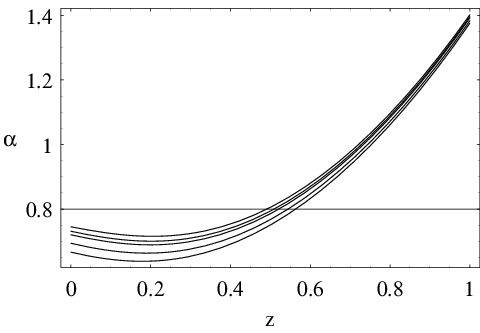
which agrees with the above analysis of the dynamical properties of this system. Here we carefully choose a new set of parameter which satisfies Friedmann constraint (39), and plot the deceleration parameter $q$ in figure 4. We see for these three set of parameters the deceleration parameters are well consistent with observations.

III perturbation growth

The Friedmann equation in the present model is given by (15). Now we consider the perturbation growth in this hybrid model. After the matter decoupling from radiation, for a region well inside a Hubble radius, the perturbation growth satisfies the following equation liddle,

\ddot{\delta}+2H\dot{\delta}-\frac{1}{6\mu^{2}}\rho_{m}\delta=0.

(41)

With the partition functions,

	$\displaystyle\Omega_{m}$	$\displaystyle=$	$\displaystyle\frac{\rho_{m}}{3\mu^{2}H^{2}},$		(42)
	$\displaystyle\Omega_{de}$	$\displaystyle=$	$\displaystyle\frac{\rho_{de}}{3\mu^{2}H^{2}},$		(43)

the perturbation equation (41) becomes,

\left(\ln\delta\right)^{\prime\prime}+\left(\ln\delta\right)^{\prime 2}+\left(2+\frac{H^{\prime}}{H}\right)\left(\ln\delta\right)^{\prime}=\frac{3}{2}\Omega_{m},

(44)

where a prime denotes the derivative with respect to $\ln a$ . $\Omega_{m}$ and $\Omega_{de}$ evolve as

	$\displaystyle\Omega_{m}=\frac{\Omega_{m0}(1+z)^{3}}{\Omega_{m0}(1+z)^{3}+\sqrt{A+B(1+z)^{6}}-\sqrt{C+D(1+z)^{6}}},$		(45)
	$\displaystyle\Omega_{de}=\frac{\sqrt{A+B(1+z)^{6}}-\sqrt{C+D(1+z)^{6}}}{\Omega_{m0}(1+z)^{3}+\sqrt{A+B(1+z)^{6}}-\sqrt{C+D(1+z)^{6}}},$		(46)

where 0 denotes the present value of a quantity. The growth function defined in (5) is just $({\ln a})^{\prime}$ . Thus (44) generates,

f^{\prime}+f^{2}+\left[\frac{1}{2}(1+\Omega_{k})+\frac{3}{2}w_{de}(\Omega_{m}+\Omega_{k}-1)\right]f=\frac{3}{2}\Omega_{m},

(47)

where we have used

\frac{H^{\prime}}{H}=-\Omega_{k}-\frac{3}{2}\left[\Omega_{m}+(1+w)\Omega_{de}\right],

(48)

and

\Omega_{m}+\Omega_{de}=1.

(49)

Recalling (5), we derive the evolution equation for $\gamma$ from (47),

3w_{de}(1-\Omega_{m})\ln\Omega_{m}\frac{d\gamma}{d\ln\Omega_{m}}+\Omega_{m}^{\gamma}-\frac{3}{2}\Omega^{1-\gamma}+3w_{de}\Omega_{m}(1/2-\gamma)+3\gamma w_{de}-\frac{3}{2}w_{de}+1/2=0,

(50)

where we have used

(\ln\Omega_{m})^{\prime}=3(1-\Omega_{m})w_{de}.

(51)

By using (8) and (9), we obtain

w_{de}=-\left[\frac{A}{\sqrt{A+B(1+z)^{6}}}-\frac{C}{\sqrt{C+D(1+z)^{6}}}\right]\left[{\sqrt{A+B(1+z)^{6}}}-\sqrt{C+D(1+z)^{6}}\right]^{-1}.

(52)

Expanding $\gamma$ about $1-\Omega_{m}$ , we get

\gamma=\frac{3}{5-w_{de}/(1-w_{de})}+2.4\times 10^{-2}(1-\Omega_{m})(1-w_{de})(1-3w_{de}/2)(1-6w_{de}/5)^{-3}.

(53)

Here we present some examples to illuminate the current numerical value of $\gamma$ in the hybrid Chaplygin gas model. We take the same examples as in figure 4. $B=0.3,~D=0.15,~\Omega_{m}=0.28$ with different $A$ and $C$ . For $A=5.92,~C=3.00$ , $\gamma=0.555$ ; for $A=1.63,~C=0.300$ , $\gamma=0.553$ ; for $A=1.01,~C=0.0300$ , $\gamma=0.550$ . The theoretical values of this model are well consistent with observations growth1; growth2; growth3; growth4; growth5; growth6; growth7; growth8; growth9; growth10; growth11; growth12; growth13; growth14.

IV Conclusion and discussion

Through careful analysis, we find a new kind of Chaplygin gas , called type II Chaplygin gas, whose energy density is negative. Then we present a hybrid Chaplygin gas model, in which type I Chaplygin gas and type II Chaplygin gas play the role of dark energy together. The EOS of dark energy crosses $-1$ naturally without introducing any gravity theories.

In frame of standard general relativity and a spatially flat FRW universe, we study the dynamical properties of the present model. We find attractor solutions both in the early universe and the late time universe: The former greatly mitigates the coincidence problem, while the latter overcomes big rip disaster. The stability about the singularities is also investigated.

Some concrete examples of the deceleration parameter of this model are plotted. The result is well consistent with observations. Also because this model is definitely free of any extra difficulties from CMB decoupling, the structure formation can be studied in frame of it.

We discuss the perturbation growth of this model. We find that the result is also consistent with observations.

Acknowledgments. We thank Z. Guo for helpful discussions. This work was supported by the National Natural Science Foundation of China , under Grant No. 10533010, and by SRF for ROCS, SEM of China.

References

(1) A. G. Riess et al., Astron. J. 116, 1009 (1998), astro-ph/9805201.
(2) S. Perlmutter et al., Astrophys. J. 517, 565 (1999), astro-ph/9812133.
(3) E. J. Copeland, M. Sami and S. Tsujikawa, Int. J. Mod. Phys. D 15, 1753 (2006) [arXiv:hep-th/0603057].
(4) A. Kamenshchik, U. Moschella and V. Pasquier, Phys. Lett. B511 (2001) 265.
(5) N. Bilic, G.B. Tupper and R.D. Viollier, Phys. Lett. B535 (2002) 17.
(6) N. Bilic, G.B. Tupper and R.D. Viollier, astro-ph/0207423.
(7) M. Bordemann and J. Hoppe, Phys. Lett. B317 (1993) 315.
(8) J.C. Fabris, S.V.B. Gonsalves and P.E. de Souza, Gen. Rel. Grav. 34 (2002) 53.
(9) M.C. Bento, O. Bertolami and A.A. Sen, Phys. Lett. B575 (2003) 172.
(10) M. Makler, S.Q. de Oliveira and I. Waga, Phys. Lett. B555 (2003) 1.
(11) J.C. Fabris, S.V.B. Goncalves and P.E. de Souza, astro-ph/0207430.
(12) Y. Gong and C.K. Duan, Class. Quant. Grav. 21 (2004) 3655.
(13) Y. Gong, JCAP 0503 (2005) 007.
(14) M.C. Bento, O. Bertolami and A.A. Sen, Phys. Rev. D67 (2003) 063003.
(15) Z.H. Zhu, Astron.Astrophys. 423 (2004) 421, astro-ph/0411039.
(16) H. Sandvik, M. Tegmark, M. Zaldarriaga, I. Waga, Phys.Rev. D69 (2004) 123524, astro-ph/0212114.
(17) M. C. Bento, O. Bertolami and A. A. Sen, Phys. Rev. D 70, 083519 (2004) ,astro-ph/0407239.
(18) P. P. Avelino, L. M. G. Beca, J. P. M. de Carvalho and C. J. A. Martins, JCAP 0309, 002 (2003),astro-ph/0307427.
(19) N. Bilic, R. J. Lindebaum, G. B. Tupper and R. D. Viollier, JCAP 0411, 008 (2004).
(20) T. M. Davis et al., Astrophys. J. 666, 716 (2007) [arXiv:astro-ph/0701510].
(21) H. K. Jassal, J. S. Bagla and T. Padmanabhan, arXiv:astro-ph/0601389.
(22) Kyle M. Wilson, Gang Chen and Bharat Ratra, Mod.Phys.Lett. A21 (2006) 2197.
(23) E. Komatsu et al. [WMAP Collaboration], arXiv:0803.0547 [astro-ph].
(24) U. Alam, V. Sahni, T. D. Saini and A. A. Starobinsky, Mon. Not. Roy. Astron. Soc. 354, 275 (2004) astro-ph/0311364
(25) U. Alam, V. Sahni and A. A. Starobinsky, JCAP 0406, (2004) 008, astro-ph/0403687.
(26) D. Huterer and A. Cooray, astro-ph/0404062.
(27) Y. Wang and M. Tegmark, astro-ph/0501351.
(28) Yun Wang, Pia Mukherjee,astro-ph/0703780.
(29) Z. K. Guo, Y. S. Piao, X. Zhang and Y. Z. Zhang, arXiv:astro-ph/0608165.
(30) B. Feng, X. L. Wang and X. M. Zhang, Phys. Lett. B 607, 35 (2005) [arXiv:astro-ph/0404224].
(31) M. R. Setare, Phys. Lett. B 641, 130 (2006).
(32) X. Zhang, Phys. Rev. D 74, 103505 (2006) [arXiv:astro-ph/0609699].
(33) M. Alimohammadi and H. M. Sadjadi, arXiv:gr-qc/0608016.
(34) H. Mohseni Sadjadi and M. Alimohammadi, Phys. Rev. D 74, 043506 (2006) [arXiv:gr-qc/0605143].
(35) W. Wang, Y. X. Gui and Y. Shao, Chin. Phys. Lett. 23 (2006) 762.
(36) X. F. Zhang and T. Qiu, arXiv:astro-ph/0603824.
(37) R. Lazkoz and G. Leon, Phys. Lett. B 638, 303 (2006) [arXiv:astro-ph/0602590].
(38) X. Zhang, Commun. Theor. Phys. 44, 762 (2005).
(39) P. x. Wu and H. w. Yu, Int. J. Mod. Phys. D 14, 1873 (2005) [arXiv:gr-qc/0509036].
(40) G. B. Zhao, J. Q. Xia, M. Li, B. Feng and X. Zhang, Phys. Rev. D 72, 123515 (2005) [arXiv:astro-ph/0507482].
(41) H. Wei, R. G. Cai and D. F. Zeng, Class. Quant. Grav. 22, 3189 (2005) [arXiv:hep-th/0501160].
(42) H. Wei and R. G. Cai, Phys. Rev. D 72 (2005) 123507 [arXiv:astro-ph/0509328].
(43) H. Wei and R. G. Cai, Phys. Lett. B 634, 9 (2006) [arXiv:astro-ph/0512018].
(44) J. Q. Xia, B. Feng and X. M. Zhang, Mod. Phys. Lett. A 20, 2409 (2005) [arXiv:astro-ph/0411501].
(45) Z. K. Guo, Y. S. Piao, X. M. Zhang and Y. Z. Zhang, Phys. Lett. B 608, 177 (2005) [arXiv:astro-ph/0410654].
(46) B. Feng, M. Li, Y. S. Piao and X. Zhang, Phys. Lett. B 634, 101 (2006) [arXiv:astro-ph/0407432].
(47) X. Zhang and F.Q. Wu, Phys. Rev. D72 (2005) 043524.
(48) Y.-F. Cai, H. Li, P.-S. Piao and X. M. Zhang, Phys. Lett. B646, 141 (2007) [arXiv:gr- qc/0609039].
(49) R. Lazkoz and G. Leon, Phys. Lett. B 638, 303 (2006) [arXiv:astro-ph/0602590].
(50) H. Wei and R. G. Cai, Phys. Rev. D 73, 083002 (2006).
(51) R. G. Cai, H. S. Zhang and A. Wang, Commun. Theor. Phys. 44, 948 (2005) [arXiv:hep-th/0505186].
(52) A.A. Andrianov, F. Cannata and A. Y. Kamenshchik, Phys.Rev.D72, 043531(2005).
(53) F.Cannata and A. Y. Kamenshchik ,gr-qc/0603129.
(54) Pantelis S. Apostolopoulos and Nikolaos Tetradis ,Phys. Rev. D 74 (2006) 064021.
(55) H. S. Zhang and Z. H. Zhu, Phys. Rev. D 75, 023510 (2007) [arXiv:astro-ph/0611834].
(56) Y.-F. Cai, M. Li, J.-X. Lu, Y.-S. Piao, T. T. Qiu and X. M. Zhang, arXiv:hep- th/0701016.
(57) N. D. Birrell & P. C. Davies, ¡°Quantum Fields In Curved Space,¡± Cambridge Univ. Press,1982.
(58) R.R. Caldwell, Phys.Lett. B545 (2002) 23, astro-ph/9908168.
(59) H. S. Zhang and Z. H. Zhu, Phys. Rev. D 73, 043518 (2006).
(60) R. R. Caldwell, M. Kamionkowski and N. N. Weinberg, Phys. Rev. Lett. 91, 071301 (2003) [arXiv:astro-ph/0302506].
(61) E. V. Linder, Phys. Rev. D 72, 043529 (2005) [astro-ph/0507263];
(62) D. Huterer and E. V. Linder, Phys. Rev. D 75, 023519 (2007) [astro-ph/0608681];
(63) L. M. Wang and P. J. Steinhardt, Astrophys. J. 508, 483 (1998) [astro-ph/9804015];
(64) Y. Wang, arXiv:0710.3885 [astro-ph].
(65) Y. Wang, arXiv:0712.0041 [astro-ph].
(66) M. Kunz and D. Sapone, Phys. Rev. Lett. 98, 121301 (2007) [astro-ph/0612452];
(67) S. Wang, L. Hui, M. May and Z. Haiman, Phys. Rev. D 76, 063503 (2007) [arXiv:0705.0165].
(68) A. Cardoso, K. Koyama, S. S. Seahra and F. P. Silva, arXiv:0711.2563 [astro-ph];
(69) K. Koyama, Gen. Rel. Grav. 40, 421 (2008) [arXiv:0706.1557].
(70) A. Lue, R. Scoccimarro and G. D. Starkman, Phys. Rev. D 69, 124015 (2004) [astro-ph/0401515].
(71) C. Di Porto and L. Amendola, arXiv:0707.2686 [astro-ph].
(72) L. Amendola, M. Kunz and D. Sapone, arXiv:0704.2421 [astro-ph].
(73) D. Sapone and L. Amendola, arXiv:0709.2792 [astro-ph].
(74) D. Polarski and R. Gannouji, Phys. Lett. B 660, 439 (2008) [arXiv:0710.1510].
(75) P. J. E. Peebles, Large-Scale Structure of the Universe, Princeton University Press, Princeton, 1980.
(76) B. Ratra and P. J. E. Peebles, Phys. Rev. D 37, 3406 (1988).
(77) P. J. E. Peebles and B. Ratra, Astrophys. J. 325, L17 (1988).
(78) L. M. Wang and P. J. Steinhardt, Astrophys. J. 508, 483 (1998) [astro-ph/9804015].
(79) Z. K. Guo and Y. Z. Zhang, Phys. Rev. D 71, 023501 (2005) [arXiv:astro-ph/0411524].
(80) A Liddle and D Lyth, The cosmological inflation and large-scale structure, Cambrige University Press, Cambrige, 2000.