Holographic Electroweak Symmetry Breaking from D-branes Preprint: WM-07-102
Abstract
We observe several interesting phenomena in a technicolor-like model of electroweak symmetry breaking based on the D4-D8-system of Sakai and Sugimoto. The benefit of holographic models based on D-brane configurations is that both sides of the holographic duality are well understood. We find that the lightest technicolor resonances contribute negatively to the Peskin-Takeuchi -parameter, but heavy resonances do not decouple and lead generically to large, positive values of , consistent with standard estimates in QCD-like theories. We study how the parameter and the masses and decay constants of the vector and axial-vector techni-resonances vary over a one-parameter family of D8-brane configurations. We discuss possibilities for the consistent truncation of the theory to the first few resonances and suggest some generic predictions of stringy holographic technicolor models.
I Introduction
In recent years, the holographic relationship between strongly-coupled field theories and higher-dimensional theories that include gravity (the AdS/CFT correspondence AdSCFT) has allowed quantitative predictions for observables in QCD that are in surprisingly good agreement with the experimental data AdSQCD1; AdSQCD2; AdSQCD3; Erdmenger; Evans. Encouraged by the success of such models, a similar approach to studying technicolor-like models of electroweak symmetry breaking (EWSB) based on the AdS/CFT correspondence has led to new possibilities for physics that may be probed at the Large Hadron Collider (LHC) Holo-EWSB1; Holo-EWSB2; CET; piai2. Holographic technicolor models are closely related to extra-dimensional models of electroweak symmetry breaking that have been studied in much detail recently EWSB-models, but their philosophy is different. In the AdS/CFT approach, the form of the 5D holographic theory is suggested by the mechanisms of chiral symmetry breaking and confinement as they appear in string theory constructions of models similar to QCD.
One benefit of holographic models rooted in D-brane configurations of string theory, as opposed to in the phenomenological models of Refs. Holo-EWSB1; Holo-EWSB2; CET; piai2, is that the large- and curvature corrections, for example, are well defined and can, in principle, be calculated or estimated systematically. Furthermore, the gauge theories described by low-energy fluctuations of D-brane configurations are known, so that both sides of the holographic duality are well understood. The stringy model of this sort most similar to the light quark sector of QCD is the D4-D8-model of Sakai and Sugimoto SS1; SS2, which we review in Section II. The Sakai-Sugimoto model is nonsupersymmetric, contains flavors of massless quarks transforming in the fundamental representation of the SU gauge group, and is confining with non-Abelian chiral symmetry breaking. (A related model based on D6-branes rather than D8-branes does not have this last feature Mateos.) At large and large ’t Hooft coupling with , the spectrum of resonances, their decay widths and couplings can be reliably calculated SS1; SS2.
Minimal technicolor models are essentially scaled up versions of QCD, in which an SU(2)U(1) subgroup of the chiral symmetry is gauged. Chiral symmetry breaking due to the strong technicolor interactions then translates into electroweak symmetry breaking. A nice feature of technicolor models is that they avoid the hierarchy problem associated with scalar Higgs fields. To produce fermion masses, however, the technicolor sector must be extended, and it is challenging to accommodate a heavy top quark in such models while avoiding large flavor-changing neutral current effects. Also disappointing is that corrections to precision electroweak observables are estimated to be generically too large to be consistent with LEP data PT. Walking technicolor models, with couplings that run more slowly than in QCD, provide one approach to solving these problems (see, for example, Refs. walking).
If the electroweak subgroup of the chiral symmetry in the Sakai-Sugimoto model is gauged, then the model becomes a technicolor-like model of electroweak symmetry breaking. The Sakai-Sugimoto model has, in addition to , and the ’t Hooft coupling, a free parameter , not present in QCD, that fixes the D8-brane configuration. (The definition of is given in Section II.) We can therefore hope that for some choice of the model will be consistent with precision electroweak constraints. Indeed, in phenomenological holographic technicolor models, additional parameters not present in QCD allow for corrections to precision electroweak observables that render them consistent with current bounds Holo-EWSB1; Holo-EWSB2; CET; piai; agashe. The Sakai-Sugimoto model also includes a larger group of symmetries (a global SO(5) symmetry) and states (Kaluza-Klein modes around a circle of size comparable to the confining scale) not present in QCD. The existence of these additional states may be considered a prediction of the model. We find it interesting that in calculable string theory models with chiral symmetry breaking it seems to be difficult to separate additional physics from the confining scale. In our adaptation of the Sakai-Sugimoto model to EWSB, one expects technicolor-like resonances to be discovered together with Kaluza-Klein modes of a large extra dimension.
The most serious problem for old-fashioned technicolor models is the generically large value of the Peskin-Takeuchi -parameter, which parameterizes a class of corrections to precision electroweak observables PT. In Section III, we calculate several of the lightest vector and axial vector resonance masses, their decay constants, and their contribution to the -parameter, as a function of (the free parameter in the model) for fixed and . We find that the contribution of the lightest resonances to is negative, which would seem to make such models promising candidates for a theory of EWSB. However, we also sum over all modes via a holographic sum rule and demonstrate a surprising non-decoupling of heavy resonances. The non-decoupling of contributions to the -parameter is a consequence of the rapid growth of the decay constants as a function of resonance number, which offsets the suppression from the increase in resonance masses. Including the effects of the entire tower of resonances, we find that the -parameter in the model is generally large and positive.
The decoupling of the heavier resonances can be recovered if we introduce an artificial ultraviolet (UV) regulator that brings the D8-brane boundary in from infinity. Although only the first few resonances are required in this limit to accurately compute , we then find that their contribution typically becomes positive and large. For regulator scales lower than the weak scale, we show that it is possible to obtain positive values of consistent with current bounds. We discuss the phenomenological implications of these results, and other approaches to decreasing the parameter, in Section IV.
II The D4-D8- System
The D4-D8-system of Sakai and Sugimoto SS1; SS2 is similar to QCD in many ways. If there are D4 branes and sets of D8 and branes, then the D-brane configuration describes an SU() gauge theory coupled to flavors of fermions in the fundamental representation, which we will refer to as either quarks or techniquarks depending on the context. The D4 branes are wrapped on a circle; antiperiodic boundary conditions for the fermions break supersymmetry and lift the masses of the extraneous (adjoint) fermions. The quarks experience chiral symmetry breaking and confinement, as is qualitatively understood by properties of the D8-brane configuration and the background geometry. Properties of the hadronic bound states (masses, decay rates and couplings) in this system are calculable, as we review here.
The D4 brane geometry, in the notation of SS1 (except for the signature of the metric), is given by,
| (1) |
where
| (2) |
The D4 brane extends in the and directions, where the direction is compactified on a circle. In the remaining dimensions, the metric is spherically symmetric: is the radial coordinate and is the metric of the unit 4-sphere. The scale is a free parameter, but to avoid a singularity at the variable is periodic with period . We will refer to the geometry projected onto the and directions as the -tube, illustrated in Fig. 1. The D8 and branes extend in the and 4-sphere directions, and follow a minimal energy trajectory on the -tube. Physical results will depend on and in the combination,
| (3) |
so that there is a single dimensionful scale, , governing the dynamics of the model. The boundary of the spacetime is at , which is topologically , where is 3+1 dimensional Minkowski space (with the Lorentz invariance of the 4D theory). The dilaton appears in the Dirac-Born-Infeld (DBI) action governing the dynamics of the D8 branes; in the D4 brane background the dilaton profile is,
| (4) |
The RR four-form is also turned on in the D4-brane background, but we will not need its profile in what follows.
Confinement in the model is related to the termination of the geometry at , i.e. the restriction . One way to understand confinement in this context is to consider a string stretched from the boundary at one point in to another as a function of separation of the string endpoints. The minimum energy string extends away from the boundary, and for large enough separation between string endpoints, will stretch all the way to . For still larger separation, the string stretches from infinity along the -tube to , moves along , and returns to . The motion along at roughly fixed gives a contribution to the energy of the string proportional to the separation of the endpoints along . This linear potential is a signature of confinement.
One striking difference between QCD and the Sakai-Sugimoto model is that the latter predicts additional Kaluza-Klein (KK) modes associated with the compact dimensions. Notably, sets both the confinement scale and the mass scale of the KK modes; above the confining scale, the additional dimension parameterized by the coordinate becomes apparent. While it is common to ignore the Kaluza-Klein modes, and assume that only the 4D model of the lowest modes is realistic, we consider the existence of these Kaluza-Klein excitations as a prediction of holographic EWSB. Thus, we expect a tower of heavy gauge bosons to appear in addition to technicolor-like resonances. The D4-D8-configuration also has an SO(5) symmetry from the 4-sphere directions, which becomes an SO(5) global symmetry in the field theory, leading to additional KK modes.
In order to decouple string loop () and gravity () corrections, and are taken to be large. In the probe brane limit, (first introduced in the context of the D3-D7 system by Karch and Katz KK), the D4 branes generate a spacetime geometry in which stable D8 brane configurations minimize their action. This is the easiest case to study, as the backreaction on the geometry due to the D8 branes can be ignored. The D8-brane configurations in the D4-D8-system were worked out in Refs. SS1 and Aharony. It was found that the D8 and branes (which are otherwise distinguished by their orientation) join at some . The D8-profile is determined by minimizing the Dirac-Born-Infeld action with gauge fields on the branes turned off,
| (5) |
where is the induced metric on the D8-branes. The result of minimizing this action is Aharony,
| (6) |
For the solution with , the D8-branes stretch from antipodal points along the circle at to the tip of the -tube at , as in Fig. 1a. Generic D8-configurations are sketched in Fig. 1b.
For the solutions with the asymptotic distance along the circle between the D8 and branes as is found to be Aharony
| (7) |
The value of is plotted as a function of in Fig. 2.

The induced metric on the D8-configuration is obtained by eliminating in favor of in Eq. (1) using Eq. (6):
| (8) |
The determinant of the induced metric is then
| (9) |
The connection of the branes at signals the breaking of the SUSU chiral symmetry of the 4+1 dimensional theory (or correspondingly the gauge invariance on the D8 branes) to an SU subgroup. Quarks in this theory are massless because the D8 branes and D4 branes cannot be separated: the D8 branes are codimension 1 and the D4 branes extend in the transverse direction. Chiral symmetry breaking is associated with the formation of a quark condensate, although it is difficult to ascertain its exact value as a function of . (If the quark mass were nonvanishing, one could vary the action with respect to it to obtain the condensate, as in Ref. Mateos. For nonvanishing quark masses in D8-brane scenarios, see Ref. quarkmass.) On the other hand, the technipion decay constant can be estimated holographically, as we describe in the next section, and is fixed to GeV in order to reproduce the spectrum of electroweak gauge bosons (or to MeV to reproduce the pion decay constant in QCD). In QCD, the confinement and chiral symmetry breaking scales are related to one another, as is the case in the D-brane construction. However, in the D4-D8-model there is an additional parameter, , that does not correspond to any parameter in QCD. The ratio of the chiral symmetry breaking scale to the confinement scale varies as a function of the free parameter, as noticed in Ref. Harvey.
III Holographic Technicolor from the D4-D8- System
In technicolor models, a new set of asymptotically free gauge interactions are postulated under which the Standard Model particles are neutral. Fermions charged under both the technicolor and electroweak interactions condense due to strong technicolor dynamics and break the electroweak gauge group to the U(1) gauge invariance of electromagnetism. Just as hadrons appear as bound states of confined quarks and gluons, technihadrons are predicted to exist as bound states of techniquarks and technigluons. The properties of technihadrons are difficult to calculate for the same reason that the properties of hadrons in QCD are difficult to calculate: the interactions are strong at the low energies of interest. However, in holographic models it is straightforward to estimate masses, decay rates and couplings of hadronic resonances. In QCD, the chiral symmetry of the light quarks is broken to a diagonal subgroup, yielding a spectrum of Goldstone bosons that we refer to generically as pions. In technicolor models, an SU(2)U(1) subgroup of the chiral symmetry is gauged and identified with the electroweak gauge group. With two techniquark flavors, the would-be pions are eaten by the and boson and do not appear as physical states in the spectrum. However, techni-vector () resonances and techni-axial vector () resonances are expected to be present, and are a generic prediction of technicolor models.
In phenomenological models of EWSB based on the AdS/CFT correspondence, it has been found that corrections to precision electroweak observables can be suppressed by adjusting available parameters Holo-EWSB1; Holo-EWSB2; CET; piai. There are even scenarios in which the -parameter is negative Holo-EWSB2, although there is some debate as to whether scenarios leading to negative can be physically realized Holo-EWSB1; csaba. A disadvantage to the phenomenological approach is that it is not known whether an ordinary quantum field theory interpretation of those models is always possible. On the other hand, models based on actual D-brane configurations avoid this problem: the appropriate field theory description is that of low-energy fluctuations on the given D-brane configuration. Unfortunately, the AdS/CFT correspondence is most powerful as a calculational tool in limits of the parameters that may not be physically relevant. In particular, in the supergravity limit it is assumed that and are large, so that gravity and stringy effects are decoupled from the field theory that lives on the D-branes. As a result of the large- limit, the resonances are infinitely narrow in a spectral decomposition of correlation functions, an outcome that is generic in holographic models if higher dimensional loop corrections are not taken into account.
One of the most serious problems for technicolor models is their generically large value of the Peskin-Takeuchi -parameter PT. The parameter can be defined in terms of matrix elements of the vector current and axial-vector current two-point functions PT:
| (10) |
| (11) |
where . From a dispersive representation with delta function resonances, the current two-point functions can be expressed in terms of the resonance masses and decay constants (up to constant local counterterms) yielding
| (12) |
It then follows that the parameter can be written as a sum over the vector and axial vector resonances as
| (13) |
The spectrum and decay constants of the lightest few hadronic resonances in the Sakai-Sugimoto model for the configuration in which the D8-branes stretche between antipodal points on the circle were calculated in Ref. SS2. The extension of these results to other D8-brane configurations was described in Ref. Aharony, although the purpose of that paper was to study finite temperature physics, and numerical solutions for the resonance masses and decay constants were not computed. The analysis is similar to that for the D4-D6- system in Ref. Mateos.
To calculate the decay constants and , and masses and , one studies the DBI action on the probe D8-branes,
| (14) |
where is the gauge field strength on the D8 branes, , and is the induced metric, Eq. (8). The determinant is over the Lorentz matrix structure, and traces over the gauge group in the expansion of the determinant are to be understood. There is a Chern-Simons term in the D8-brane action which we consistently ignore, since we restrict our attention to terms only quadratic in the gauge fields. The integral is over twice: once over the D8 brane segment and once over the brane segment. We only study configurations constant along the and such that for . From a 5D perspective, the remaining modes are related to these by the SO(5) symmetry of the brane configuration, plus a set of scalar fields from the decomposition of the gauge fields around the 4-sphere. Expanding the action to quadratic order in ,
| (15) | |||||
where , is the area of the unit 4-sphere, and contractions of indices are with respect to the 5D Minkowski metric. We have defined the function as in Ref. Aharony:
| (16) |
Expanding in modes, the vector modes are symmetric upon reflection about while the axial vector modes are antisymmetric. These modes are identified with the tower of vector and axial vector mesons in the 4+1 dimensional gauge theory, with the circle dimension suppressed. The normalizable modes satisfy Dirichlet boundary conditions: on both the D8 and branches of the -segment . The symmetric solutions also satisfy , while the antisymmetric modes satisfy .
Note that in the coordinate system one must consider two branches of , the D8-brane branch and the -brane branch. The branes meet at so we sometimes refer simply to the D8-brane configuration. To simplify the discussion of boundary conditions we will sometimes find it convenient to change coordinates, for example to defined by , , which covers both branches of the D8-configuration. Since the equations of motion are more cumbersome in such coordinate systems, unless , we will use the coordinate in most of what follows.
We will work in a gauge in which . As in Ref. SS2, we expand the vector field in normalizable modes satisfying Dirichlet boundary conditions =0:11 1 Since we are interested in the case we should be careful not to fall prey to the Witten anomaly. To be precise, the boundary condition is that the gauge fields are pure gauge at infinity, and such configurations fall into one of two classes (because ). This subtlety will not affect any of our results, and we simply note that we must assume the techniquarks transform under an even-dimensional representation of the technicolor group to have a well-defined theory.
| (17) |
The are the symmetric modes, and are antisymmetric. The equations of motion are
| (18) |
and similarly for the axial vector modes with . The spectrum alternates between symmetric and antisymmetric modes, so that the vector and axial vector masses alternate, as in Fig. 3.

A source for the SU(2)L or SU(2)R current corresponds to a non-normalizable solution to the equation of motion for localized near either the D8 or brane boundary, respectively. Similarly, a source for SU(2)V corresponds to a non-normalizable solution symmetric around , while a source for SU(2)A corresponds to an anti-symmetric configuration. We will call the symmetric non-normalizable solutions, Fourier transformed in the coordinates , , where on both branches of . We call the antisymmetric solutions , where on the D8 brane branch and on the branch. The gauge transformation which sets reappears in the sources and and gives rise to the pion kinetic terms and couplings, as discussed in SS2. For our purposes it will be good enough to set these pion degrees of freedom to zero. They will get eaten after gauging of the electroweak subgroup of the chiral symmetry, in any case. The bulk-to-boundary propagators and satisfy the equation of motion (18) with replaced by . A general decomposition of the gauge fields into normalizable modes in addition to a source for the SU(2)SU(2) current is then
| (19) |
Up to gauge fixing terms, the decomposition of the action, Eq. (15), to quadratic order in the gauge fields is given by
| (20) | |||||
If the SU generators are normalized so that Tr , then the gauge fields are canonically normalized if:
| (21) | |||
| (22) |
It is natural to define, as in Ref. SS2,
| (23) |
where we have used the relations SS1:
| (24) |
Using the equations of motion Eq. (18) we can write the action in terms of the canonically normalized modes as
| (25) | |||||
where
| (26) |
is the kinetic term for the sources and , and is given by,
| (27) |
The constants and are given by,
| (28) |
We have used the equations of motion and boundary conditions on , , and to eliminate vanishing surface terms, e.g.,
| (29) | |||||
and similarly for .
Diagonalizing the kinetic terms, we obtain the action,
| (30) | |||||
where
| (31) |
is the gauge kinetic term for , and similarly for . The kinetic term for the source picks up an additional contribution in this process. From the coupling between the sources and the modes we identify the decay constants,
| (32) | |||||
The decay constants grow with as the masses do, as demonstrated in Fig. 4.

The spectrum of the lightest four vector and axial vector resonances, and their decay constants, were given in Ref. SS2 for the antipodal D8-configuration . The contribution of the first four pairs of resonances to the parameter Eq. (11) using the results of Ref. SS2 is , where in the last approximation we set and . The lightest pair of resonances contributes negatively to the -parameter. In fact, the three-digit precision to which the results in Ref. SS2 are quoted is not good enough for this calculation because of the propagation of errors in summing over the small differences between the large contributions of the vector and axial vector modes to . We find by increasing the precision of our numerical calculation that , larger by an order of magnitude than our estimate from Sakai and Sugimoto’s results. It is clear that the contributions from individual sets of modes to the parameter are sensitive to the details of the model. Increasing the parameter makes the contribution of the lightest modes to the -parameter even more negative, as seen in Fig. 5.

On the other hand, we can also calculate the -parameter exactly (in the large limit) by using the bulk-to-boundary propagators and , analogous to the derivation of the sum rules in Ref. sumrules. It is convenient to temporarily employ a coordinate that spans both the D8 and branches,
| (33) |
where () corresponds to the D8 brane (brane). In momentum space, the vector bulk-to-boundary propagator satisfies
| (34) |
with at . We aim to relate this to the following Green’s function for the equation of motion operator
| (35) |
where we assume Dirichlet boundary conditions . It follows from the normalization condition for the modes, Eq. (21), that we may rewrite the delta function in Eq. (35) using the completeness relation
| (36) |
If we then apply the ansatz
| (37) |
one can extract the coefficients from Eq. (35) by application of the equations of motion. It follows that may be expressed as a sum over modes,
| (38) |
For definiteness, let us consider the relationship between and the bulk-to-boundary propagator of the vector modes . We begin with the identity
| (39) |
Replacing the delta function using Eq. (35), one may integrate by parts twice to show that the right-hand-side of Eq. (39) is a surface term
| (40) |
where we have defined . In terms of the mode decomposition, contains only those modes that are even under reflection about (i.e., ), which we called earlier:
| (41) |
The form of this result is suggestive: is precisely the same as the quantity that appeared in our holographic expressions for the decay constants, Eqs. (32). We now take a derivative of each side with respect to and take the limit . We may re-express the derivatives of the wave functions appearing in Eq. (41) in terms of decay constants, for . However, the sum is convergent only when one takes the limit with . The difference between the limit of the sum and its value at the limit point is a divergent quantity , such that
| (42) |
where primed quantities are functions of , or in original coordinates,
| (43) |
Sums that involve higher powers of in the denominator are convergent, which suggests that is a constant independent of . This can be shown by taking derivatives in Eq. (41), so that the sum is convergent and there is no ambiguity in the evaluation of the subsequent limits, and comparing to the same derivatives of Eq. (43). We fix by noting that is a constant, so that the right-hand-side of Eq. (43) vanishes in the limit ; it follows that
| (44) |
The left-hand-side of Eq. (43) may now be combined to give precisely defined in Eq. (12),
| (45) |
To obtain the axial-vector self-energy, , one must take into account that the axial bulk-to-boundary propagator satisfies the boundary conditions and . One can then derive an expression of the same form as Eq. (43) with , , and replaced by , , and , respectively. The evaluation of , however, is different in this case. One can show that the right-hand-side of the axial version of Eq. (43) evaluates to a non-vanishing constant when , which we identify with the square of the pion decay constant, . Indeed, we find that when this constant agrees with the prediction as determined in Refs. SS1; SS2 by studying the pion part of the effective action. Thus we set
| (46) |
and
| (47) |
Using the definition of the parameter given in Eq. (11), it immediately follows that
| (48) |
This result represents a sum over all resonances. We find that Eq. (48) leads to large, positive that increases with , a surprising result given the behavior shown in Fig. 5. We explore this issue further in the next section. For the antipodal D8-configuration we obtain
| (49) |
where have again taken and for the numerical evaluation. This is a factor of larger than the estimate of in a one-doublet, SU(4) technicolor models with QCD-like dynamics PT. As a function of we plot the parameter in Fig. 6.

It is worth noting that the scale , with respect to which we have been measuring masses and decay constants, is determined by the electroweak scale
| (50) |
where is given by Eq. (47). Eq. (50) is simply one of the Weinberg sum rules with the renormalization condition , as is satisfied by Eq. (45). This expression for can also be derived by studying the two-point coupling of the axial vector source to the pion field, as in Ref. SS2. As noted earlier, we have set the pion field to zero in our analysis. In the model with we find that , in agreement with Refs. SS1; SS2. Hence, in that model GeV TeV, where in the last approximation we set and . sets the scale of additional Kaluza-Klein states in the spectrum. also sets the scale of the technihadrons: in the same approximation we find that the lightest technirho has mass TeV; and the lightest techni-axial vector has mass TeV. Note that once the electroweak scale is fixed, the only remaining freedom in the model in addition to and is the one-parameter choice of D8-brane configuration. Although we have found that the parameter is too large in this model to be a consistent model of EWSB, the couplings between technicolor resonances and additional phenomenology can be calculated in the model to the same accuracy as the calculations above. We turn our attention to ways in which the parameter prediction of our model might be reduced in the next section.
It is also worth noting that we can derive the above relations for and by the usual AdS/CFT prescription of varying the action with respect to the sources for the currents and . In particular, the term in proportional to is obtained by varying , with given in Eq. (27), with respect to twice, using the equations of motion. (The transverse tensor structure can be obtained by keeping track of gauge fixing terms, as in AdSQCD3.) The result is,
| (51) |
Comparing with Eq. (28) we see that the AdS/CFT procedure has successfully reproduced our result, Eq. (45). Similarly, we find .
IV Discussion
If we allow the D8-brane boundary to move in from infinity artificially, then the confining scale can be raised as in Refs. CET; agashe. In doing so, however, we are leaving the realm of string theory in favor of a bottom-up approach to holographic model building. Models of electroweak symmetry breaking constructed in this way have been discussed previously in Refs. Holo-EWSB1; Holo-EWSB2; CET; piai2. In our case, we may consider a 5D model motivated by the AdS/CFT correspondence, but with bulk geometry described by the induced metric on the D8-branes in the D4-D8 system. The location of the UV boundary determines the size of the radial dimension and, hence, the resonance mass scale. Since the higher resonances decouple more quickly as the size of the radial dimension is reduced, we can test the agreement of the sum over modes with the sum rule approach. Fig. 7 demonstrates the behavior of the parameter as the boundary location is varied. Here we work in the limit , and map the coordinate to a finite interval , via the relations
| (52) |
The physical boundaries at correspond to . It is clear from Fig. 7 that the lightest four pairs of vector and axial-vector modes provide a better approximation of the parameter as increases.
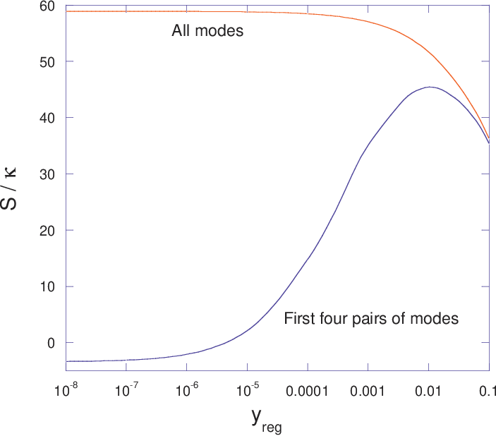
We also note that for a severely regulated theory, , the parameter can be made consistent with the current limit pdg. This corresponds to a radial dimension of proper length approximately . For the value TeV obtained in the previous section, the radial dimension has size approximately (3.6 TeV)-1.
It is interesting to note that this version of holographic duality for chiral symmetries, with two boundary components rather than the single boundary of Anti-de Sitter space, was anticipated by Son and Stephanov in Ref. Son-S. They considered a model of mesons with light-quark quantum numbers based on an extension of the notion of hidden local symmetry Bando. The model is equivalent to a deconstructed extra-dimensional SU gauge theory with an SUSU flavor symmetry corresponding to the global symmetries of the fields localized at the two boundaries. To calculate current correlators, the global symmetries are weakly gauged, and the gauge fields at the ends of the extra dimension act as sources for the currents. The configurations with SU gauge fields turned on at one boundary or the other are analogous to the non-normalizable modes localized at the boundary of the D8 brane or brane segment.
A deconstructed decons version of the Sakai-Sugimoto model would truncate the model to a finite number of resonances. Since we have found that the light resonances in the Sakai-Sugimoto model can contribute negatively to the -parameter, it would be interesting to study the behavior of the -parameter as a function of the number of lattice sites of the deconstructed model. Again, such an approach deviates from string theory since there is no simple deconstruction of the radial dimension that captures all of gravitational physics of the original theory, even in the limit of a large number of lattice sites. Nevertheless, deconstruction often leads to 4D theories that possess important features of the higher-dimensional theory that they are designed to approximate. In the present case, the Sakai-Sugimoto model would simply provide a paradigm for the choice of gauge groups and symmetry breaking pattern in the deconstructed theory. Electroweak constraints would require detailed study, especially away from the large limit where radiative corrections are generally non-negligible and must be taken into account. It would also be interesting to compare these deconstructed models with existing models of electroweak symmetry breaking that were motivated in part by deconstruction of extra dimensions, such as little Higgs models littleHiggs.
In summary, we have studied the viability of the Sakai-Sugimoto model of intersecting D4 and D8 branes as a technicolor-like model of electroweak symmetry breaking. We determined the masses of the technicolor resonances and their decay constants in terms of the electroweak scale. We found that the contribution of the strong dynamics to the Peskin-Takeuchi parameter is larger by at least an order of magnitude than the experimentally allowed value , even allowing for adjustment of the D8-brane configuration. However, we observed that the lightest pair of vector and axial vector resonances contributes negatively to , while the final result reflects a non-decoupling of heavy resonances that seems to be sensitive to the details of the model. The model can be made consistent with precision electroweak constraints by artificially introducing an ultraviolet regulator, as we showed in Fig. 7, or perhaps by deconstructing the model along the radial direction in order to truncate it to the lightest several technicolor resonances. In order to become a complete model of electroweak symmetry breaking, the Standard Model fermions would need to be included together with a mechanism for generation of their masses.
Acknowledgements.
We thank Ofer Aharony and Veronica Sanz for useful discussions. CDC thanks the NSF for support under Grant No. PHY-0456525. M.S. thanks the NSF for support under Grant No. PHY-0554854. The work of J.E. is supported in part by the NSF under Grant No. PHY-0504442 and the Jeffress Foundation under Grant No. J-768.References
- (1) J. M. Maldacena, Adv. Theor. Math. Phys. 2, 231 (1998) [Int. J. Theor. Phys. 38, 1113 (1999)] [arXiv:hep-th/9711200]; S. S. Gubser, I. R. Klebanov and A. M. Polyakov, Phys. Lett. B 428, 105 (1998) [arXiv:hep-th/9802109]; E. Witten, Adv. Theor. Math. Phys. 2, 253 (1998) [arXiv:hep-th/9802150].
- (2) G. F. de Teramond and S. J. Brodsky, Phys. Rev. Lett. 94, 201601 (2005) [arXiv:hep-th/0501022].
- (3) J. Erlich, E. Katz, D. T. Son and M. A. Stephanov, Phys. Rev. Lett. 95, 261602 (2005) [arXiv:hep-ph/0501128].
- (4) L. Da Rold and A. Pomarol, Nucl. Phys. B 721, 79 (2005) [arXiv:hep-ph/0501218].
- (5) J. Babington, J. Erdmenger, N. J. Evans, Z. Guralnik and I. Kirsch, Phys. Rev. D 69, 066007 (2004) [arXiv:hep-th/0306018].
- (6) N. Evans, J. P. Shock and T. Waterson, Phys. Lett. B 622, 165 (2005) [arXiv:hep-th/0505250].
- (7) D. K. Hong and H. U. Yee, Phys. Rev. D 74, 015011 (2006) [arXiv:hep-ph/0602177].
- (8) J. Hirn and V. Sanz, Phys. Rev. Lett. 97, 121803 (2006) [arXiv:hep-ph/0606086];
- (9) C. D. Carone, J. Erlich and J. A. Tan, Phys. Rev. D 75, 075005 (2007) [arXiv:hep-ph/0612242].
- (10) M. Piai, arXiv:0704.2205 [hep-ph].
- (11) L. Randall and R. Sundrum, Phys. Rev. Lett. 83, 3370 (1999) [arXiv:hep-ph/9905221]; N. Arkani-Hamed, S. Dimopoulos and G. R. Dvali, Phys. Lett. B 429, 263 (1998) [arXiv:hep-ph/9803315]; C. Csaki, C. Grojean, H. Murayama, L. Pilo and J. Terning, Phys. Rev. D 69, 055006 (2004) [arXiv:hep-ph/0305237]; C. Csaki, C. Grojean, L. Pilo and J. Terning, Phys. Rev. Lett. 92, 101802 (2004) [arXiv:hep-ph/0308038]; G. Cacciapaglia, C. Csaki, G. Marandella and J. Terning, arXiv:hep-ph/0611358.
- (12) T. Sakai and S. Sugimoto, Prog. Theor. Phys. 113, 843 (2005) [arXiv:hep-th/0412141].
- (13) T. Sakai and S. Sugimoto, Prog. Theor. Phys. 114, 1083 (2006) [arXiv:hep-th/0507073].
- (14) M. Kruczenski, D. Mateos, R. C. Myers and D. J. Winters, JHEP 0307, 049 (2003) [arXiv:hep-th/0304032]; M. Kruczenski, D. Mateos, R. C. Myers and D. J. Winters, JHEP 0405, 041 (2004) [arXiv:hep-th/0311270].
- (15) M. E. Peskin and T. Takeuchi, Phys. Rev. Lett. 65, 964 (1990); M. E. Peskin and T. Takeuchi, Phys. Rev. D 46, 381 (1992).
- (16) R. Sundrum and S. D. H. Hsu, Nucl. Phys. B 391, 127 (1993) [arXiv:hep-ph/9206225]; D. D. Dietrich, F. Sannino and K. Tuominen, Phys. Rev. D 72, 055001 (2005) [arXiv:hep-ph/0505059]; D. D. Dietrich, F. Sannino and K. Tuominen, Phys. Rev. D 73, 037701 (2006) [arXiv:hep-ph/0510217]; N. Evans and F. Sannino, arXiv:hep-ph/0512080.
- (17) M. Piai, arXiv:hep-ph/0609104.
- (18) K. Agashe, R. Contino and A. Pomarol, Nucl. Phys. B 719, 165 (2005) [arXiv:hep-ph/0412089].
- (19) A. Karch and E. Katz, JHEP 0206, 043 (2002) [arXiv:hep-th/0205236].
- (20) O. Aharony, J. Sonnenschein and S. Yankielowicz, arXiv:hep-th/0604161.
- (21) K. Hashimoto, T. Hirayama and A. Miwa, arXiv:hep-th/0703024.
- (22) E. Antonyan, J. A. Harvey, S. Jensen and D. Kutasov, arXiv:hep-th/0604017.
- (23) K. Agashe, C. Csaki, C. Grojean and M. Reece, arXiv:0704.1821 [hep-ph].
- (24) J. Hirn and V. Sanz, arXiv:hep-ph/0702005.
- (25) W. M. Yao et al. [Particle Data Group], J. Phys. G 33, 1 (2006).
- (26) D. T. Son and M. A. Stephanov, Phys. Rev. D 69, 065020 (2004) [arXiv:hep-ph/0304182].
- (27) M. Bando, T. Kugo, S. Uehara, K. Yamawaki and T. Yanagida, Phys. Rev. Lett. 54, 1215 (1985); M. Bando, T. Kugo and K. Yamawaki, Phys. Rept. 164, 217 (1988).
- (28) N. Arkani-Hamed, A. G. Cohen and H. Georgi, Phys. Rev. Lett. 86, 4757 (2001) [arXiv:hep-th/0104005]. C. T. Hill, S. Pokorski and J. Wang, Phys. Rev. D 64, 105005 (2001) [arXiv:hep-th/0104035]. H. C. Cheng, C. T. Hill, S. Pokorski and J. Wang, Phys. Rev. D 64, 065007 (2001) [arXiv:hep-th/0104179].
- (29) N. Arkani-Hamed, A. G. Cohen, E. Katz, A. E. Nelson, T. Gregoire and J. G. Wacker, JHEP 0208, 021 (2002) [arXiv:hep-ph/0206020]; N. Arkani-Hamed, A. G. Cohen, E. Katz and A. E. Nelson, JHEP 0207, 034 (2002) [arXiv:hep-ph/0206021];