Many-Body Physics with Ultracold Gases
Abstract
This article reviews recent experimental and theoretical progress on many-body phenomena in dilute, ultracold gases. Its focus are effects beyond standard weak-coupling descriptions, like the Mott-Hubbard-transition in optical lattices, strongly interacting gases in one and two dimensions or lowest Landau level physics in quasi two-dimensional gases in fast rotation. Strong correlations in fermionic gases are discussed in optical lattices or near Feshbach resonances in the BCS-BEC crossover.
I INTRODUCTION
The achievement of Bose-Einstein-Condensation (BEC) Anderson et al. 1995; Davis et al. 1995; Bradley et al. 1995 and of Fermi degeneracy DeMarco and Jin 1999; Truscott et al. 2001; Schreck et al. 2001 in ultracold, dilute gases has opened a new chapter in atomic and molecular physics in which the particle statistics and their interactions, rather than the study of single atoms or photons, are at center stage. For a number of years, a main focus in this field has been to explore the wealth of phenomena associated with the existence of coherent matter waves. Major examples include the observation of interference of two overlapping condensates Andrews et al. 1997, of long range phase coherence Bloch et al. 2000 or of quantized vortices and vortex lattices Madison et al. 2000; Abo-Shaeer et al. 2001 and molecular condensates with bound pairs of fermions Greiner et al. 2003; Jochim et al. 2003b; Zwierlein et al. 2003b. Common to all of these phenomena is the existence of a coherent, macroscopic matter wave in an interacting many-body system, a concept familiar from the classic area of superconductivity and superfluidity. It was the basic insight of Ginzburg and Landau 1950 that, quite independent of a detailed microscopic understanding, an effective description of the coherent many-body state is provided by a complex, macroscopic wave function . Its magnitude squared gives the superfluid density, while the phase determines the superfluid velocity via (see the Appendix for a discussion of these concepts and their subtle connection with the microscopic criterion for BEC). As emphasized by Cummings and Johnston 1966 and by Langer 1968, this picture is similar to the description of laser light by a coherent state Glauber 1963. It applies both to the standard condensates of bosonic atoms and also to weakly bound fermion pairs which are the building blocks of the BCS-picture of superfluidity in Fermi systems. In contrast to conventional superfluids like He or superconductors, where the macroscopic wave function only provides a phenomenological description of the superfluid degrees of freedom, the situation in dilute gases is considerably simpler. In fact, as a result of the weak interactions, the dilute BEC’s are essentially pure condensates sufficiently below the transition. The macroscopic wave function is thus directly connected with the microscopic degrees of freedom, providing a complete and quantitative description of both static and time-dependent phenomena in terms of a reversible, nonlinear Schrödinger-equation, the famous Gross-Pitaevskii equation Gross 1961; Pitaevskii 1961. In dilute gases therefore, the many-body aspect of a BEC is reduced to an effective single-particle description, where interactions just give rise to an additional potential proportional to the local particle density. Adding small fluctuations around this zeroth-order picture leads to the well known Bogoliubov theory of weakly interacting Bose gases. Similar to the closely related BCS-superfluid of weakly interacting fermions, the many-body problem is then completely soluble in terms of a set of non-interacting quasiparticles. Dilute, ultracold gases provide a concrete realization of these basic models of many-body physics and many of their characteristic properties have indeed been verified quantitatively. Excellent reviews of this remarkably rich area of research have been given by Dalfovo et al. 1999 and by Leggett 2001 and - more recently - in the comprehensive books by Pethick and Smith 2002 and by Pitaevskii and Stringari 2003.
In the past several years, two major new developments have considerably enlarged the range of physics which is accessible with ultracold gases. They are associated with
- •
the ability to tune the interaction strength in cold gases by Feshbach resonances Inouye et al. 1998; Courteille et al. 1998 and
- •
the possibility to change the dimensionality with optical potentials and, in particular, to generate strong periodic potentials for cold atoms through optical lattices Greiner et al. 2002a.
Both developments, either individually or in combination, allow to enter a regime, in which the interactions even in extremely dilute gases can no longer be described by a picture based on non-interacting quasi-particles. The appearance of such phenomena is characteristic for the physics of strongly correlated systems. For a long time, this area of research was confined to the dense and strongly interacting quantum liquids of condensed matter or nuclear physics. By contrast, gases - almost by definition - were never thought to exhibit strong correlations.
The use of Feshbach resonances and optical potentials for exploring strong correlations in ultracold gases was crucially influenced by earlier ideas from theory. In particular, Stoof et al. 1996 suggested that Feshbach resonances in a degenerate gas of 6Li, which exhibits a tunable attractive interaction between two different hyperfine states, may be used to realize BCS-pairing of fermions in ultracold gases. A remarkable idea in a rather unusual direction in the context of atomic physics was the proposal by Jaksch et al. 1998 to realize a quantum phase transition from a superfluid to a Mott-insulating state by loading a BEC into an optical lattice and simply raising its depth. Further directions into the regime of strong correlations were opened with the suggestions by Olshanii 1998 and Petrov et al. 2000b, to realize a Tonks-Girardeau gas with BEC’s confined in one dimension and by Wilkin and Gunn 2000 to explore quantum Hall effect physics in fast rotating gases.
Experimentally, the strong coupling regime in dilute gases was first reached by Cornish et al. 2000, using Feshbach resonances for bosonic atoms. Unfortunately, in this case, increasing the scattering length leads to a strong decrease in the condensate lifetime due to three-body losses, whose rate on average varies like Fedichev et al. 1996b; Petrov 2004. A quite different approach to the regime of strong correlations, which does not suffer from problems with the condensate lifetime, was taken by Greiner et al. 2002a. Loading BEC’s into an optical lattice, they observed a quantum phase transition from a superfluid to a Mott-insulating phase even in the standard regime where the average interparticle spacing is much larger than the scattering length. Subsequently, the strong confinement available with optical lattices made possible the achievement of low dimensional systems where new phases can emerge. In fact, the first example of a bosonic Luttinger liquid was obtained with the observation of a (Tonks-Girardeau) hard-core Bose gas in one dimension by Paredes et al. 2004 and Kinoshita et al. 2004. In two dimensions a Kosterlitz-Thouless crossover between a normal phase and one with quasi-long range order was observed by Hadzibabic et al. 2006. The physics of strongly interacting bosons in the lowest Landau level is accessible with fast rotating BEC’s Schweikhard et al. 2004; Bretin et al. 2004, where the vortex lattice is eventually predicted to melt by quantum fluctuations. Using atoms like 52Cr, which have a larger permanent magnetic moment, BEC’s with strong dipolar interactions have been realized by Griesmaier et al. 2005. In combination with Feshbach resonances, this opens the way tune the nature and range of the interaction Lahaye et al. 2007, which might, for instance, be used to reach novel many-body states that are not accessible in the context of the fractional Quantum Hall Effect.
In Fermi gases, the Pauli-principle strongly suppresses three-body losses, whose rate in fact decreases with increasing values of the scattering length Petrov et al. 2004b. Feshbach resonances therefore allow to enter the strong coupling regime in ultracold Fermi gases O’Hara et al. 2002; Bourdel et al. 2003. In particular, there exist stable molecular states of weakly bound fermion pairs, in highly excited ro-vibrational states Strecker et al. 2003; Cubizolles et al. 2003. The remarkable stability of fermions near Feshbach resonances allows to explore the crossover from a molecular BEC to a BCS-superfluid of weakly bound Cooper-pairs Regal et al. 2004a; Zwierlein et al. 2004; Bartenstein et al. 2004; Bourdel et al. 2004. In particular, the presence of pairing due to many-body effects has been probed by spectroscopy of the gap Chin et al. 2004, or the closed channel fraction Partridge et al. 2005 while superfluidity has been verified by the observation of quantized vortices Zwierlein et al. 2005. Recently, these studies have been extended to Fermi gases with unequal densities for the spin-up and spin-down components Zwierlein et al. 2006; Partridge et al. 2006, where pairing is suppressed by the mismatch of the respective Fermi energies.
Repulsive fermions in an optical lattice allow to realize an ideal and tunable version of the Hubbard model, a paradigm for the multitude of strong correlation problems in condensed matter physics. Experimentally, some of the basic properties of degenerate fermions in periodic potentials like the existence of a Fermi surface and the appearance of a band insulator at unit filling have been observed by Köhl et al. 2005a. While it is difficult to cool fermions to temperatures much below the bandwidth in a deep optical lattice these experiments give rise to the hope that eventually magnetically ordered or unconventional superconducting phases of the fermionic Hubbard model will be accessible with cold gases. The perfect control and tunability of the interactions in these systems provide a completely novel approach to study basic problems in many-body physics and, in particular, to enter regimes which have never been accessible in condensed matter or nuclear physics.
The present review aims to give an overview of this rapidly evolving field, covering both theoretical concepts and their experimental realization. It provides an introduction to the strong correlation aspects of cold gases, that is, phenomena which are not captured by weak-coupling descriptions like the Gross-Pitaevskii or Bogoliubov theory. The focus of this review is on examples which have already been realized experimentally. Even within this limitation, however, the rapid development of the field in recent years makes it impossible to give a complete survey. In particular, important subjects like spinor gases, Bose-Fermi mixtures, quantum spin systems in optical lattices or dipolar gases will not be discussed here (see e.g. Lewenstein et al. 2007). Also, applications of cold atoms in optical lattices for quantum information are omitted completely, for a recent introduction see Jaksch and Zoller 2005.
I.1 Scattering of ultracold atoms
For an understanding of the interactions between neutral atoms, first at the two-body level, it is instructive to use a toy model Gribakin and Flambaum 1993, in which the van der Waals attraction at large distances is cutoff by a hard core at some distance on the order of an atomic dimension. The resulting spherically symmetric potential
| (1) |
is, of course, not a realistic description of the short range interaction of atoms, however it captures the main features of scattering at low energies. The asymptotic behavior of the interaction potential is fixed by the van der Waals coefficient . It defines a characteristic length
| (2) |
at which the kinetic energy of the relative motion of two atoms with reduced mass equals their interaction energy. For alkali atoms, this length is typically on the order of several nano-meters. It is much larger than the atomic scale because alkalis are strongly polarizable, resulting in a large coefficient. The attractive well of the van der Waals potential thus supports many bound states (of order in 87Rb!). Their number may be determined from the WKB-phase
| (3) |
at zero energy, via where means taking the integer part11 1 This result follows from Eq. (5) below by noting that a new bound state is pulled in from the continuum each time the scattering length diverges (Levinson’s theorem).. The number of bound states in this model therefore crucially depends on the precise value of the short range scale . By contrast, the low energy scattering properties are essentially determined by the van der Waals length , which is only sensitive to the asymptotic behavior of the potential. Consider the scattering in states with angular momentum in the relative motion (for identical bosons or fermions only even or odd values of are possible, respectively). The effective potential for states with contains a centrifugal barrier whose height is of order . Converting this energy into an equivalent temperature, one obtains temperatures around mK for typical atomic masses. At temperatures below that, the energy in the relative motion of two atoms is typically below the centrifugal barrier. Scattering in states with is therefore frozen out, unless there exist so-called shape resonances, i.e. bound states with behind the centrifugal barrier, which may be in resonance with the incoming energy, see Boesten et al. 1997; Dürr et al. 2005. For gases in the sub-mK regime, therefore, usually lowest angular momentum collisions dominate (-wave for bosons, -wave for fermions), which in fact defines the regime of ultracold atoms. In the -wave case, the scattering amplitude is determined by the corresponding phase shift via Landau and Lifshitz 1987
| (4) |
At low energies, it is characterized by the scattering length and the effective range as the two single parameters. For the truncated van der Waals potential (1), the scattering length can be calculated analytically as Gribakin and Flambaum 1993
| (5) |
where is the WKB-phase (3) and the so-called mean scattering length. The expression (5) shows that the characteristic magnitude of the scattering length is the van der Waals length. Its detailed value, however, depends on the short range physics via the WKB-phase , which is sensitive to the hard core scale . Since the detailed behavior of the potential is typically not known precisely, in many cases neither the sign of the scattering length nor the number of bound states can be determined from ab initio calculations. The toy-model result, however, is useful beyond the identification of as the characteristic scale for the scattering length. Indeed, if the ignorance about the short range physics is replaced by the (maximum likelihood) assumption of a uniform distribution of in the relevant interval , the probability for finding a positive scattering length, i.e. is . A repulsive interaction at low energy, which is connected with a positive scattering length, is therefore three times more likely than an attractive one, where Pethick and Smith 2002. Concerning the effective range in Eq. (4), it turns out that also is on the order of the van der Waals or the mean scattering length rather than the short range scale as might have been expected naively 22 2 This is a general result for deep potentials with a power law decay at large distances, as long as the scattering energy is much smaller than the depth of the potential well. Flambaum et al. 1999. Since in the regime of ultracold collisions, this implies that the -contribution in the denominator of the scattering amplitude is negligible. In the low-energy limit, the two-body collision problem is thus completely specified by the scattering length as the single parameter and a corresponding scattering amplitude
| (6) |
As noted by Fermi in the context of scattering of slow neutrons and by Lee, Huang and Yang for the low temperature thermodynamics of weakly interacting quantum gases, Eq. (6) is the exact scattering amplitude at arbitrary values of for the pseudopotential 33 3 Due to the delta-function, the last term involving the partial derivative with respect to can be omitted when the potential acts on a function which is regular at .
| (7) |
At temperatures such that , two-body interactions in ultracold gases may thus be described by a pseudopotential, with the scattering length usually taken as an experimentally determined parameter. This approximation is valid in a wide range of situations, provided no longer range contributions come into play as e.g. in the case of dipolar gases. The interaction is repulsive for positive and attractive for negative scattering length. Now, as shown above, the true interaction potential has many bound states, irrespective of the sign of . For the low energy scattering of atoms, however, these bound states are irrelevant as long as no molecule formation occurs via three-body collisions. The scattering amplitude in the limit is only sensitive to bound (or virtual for ) states near zero energy. In particular, within the pseudopotential approximation the amplitude (6) has a single pole , with if the scattering length is positive. Quite generally, poles of the scattering amplitude in the upper complex -plane are connected with bound states with binding energy Landau and Lifshitz 1987. In the pseudopotential approximation, only a single pole is captured; the energy of the associated bound state is just below the continuum threshold. A repulsive pseudopotential thus describes a situation where the full potential has a bound state with a binding energy on the order of or smaller than the characteristic energy introduced above. The associated positive scattering length is then identical with the decay length of the wave function of the highest bound state. In the attractive case , in turn, there is no bound state within a range below the continuum threshold, however there is a virtual state just above it.
I.2 Weak interactions
For a qualitative discussion of what defines the weak interaction regime in dilute, ultracold gases, it is useful to start with the idealization of no interactions at all. Depending on the two fundamental possibilities for the statistics of indistinguishable particles, Bose or Fermi, the ground state of a gas of non-interacting particles is either a perfect BEC or a Fermi sea. In the case of an ideal BEC, all particles occupy the lowest available single particle level, consistent with a fully symmetric many-body wave function. For fermions, in turn, the particles fill the lowest single particle levels up to the Fermi-energy , as required by the Pauli-principle. At finite temperatures, the discontinuity in the Fermi-Dirac distribution at is smeared out, giving rise to a continuous evolution from the degenerate gas at to a classical gas at high temperatures . By contrast, bosons exhibit in 3D a phase transition at finite temperature, where the macroscopic occupancy of the ground state is lost. In the homogeneous gas, this transition occurs when the thermal de Broglie wavelength reaches the average interparticle distance . The surprising fact that a phase transition appears even in an ideal Bose gas is a consequence of the correlations imposed by the particle statistics alone, as noted already in Einstein’s fundamental paper Einstein 1925. For trapped gases, with geometrical mean trap frequency , the transition to a BEC is in principle smooth44 4 A Bose gas in a trap exhibits a sharp transition only in the limit with , i.e. when the critical temperature approaches a finite value in the thermodynamic limit.. Yet, for typical particle numbers in the range , there is a rather sharply defined temperature , above which the occupation of the oscillator ground state is no longer of order . This temperature is again determined by the condition that the thermal de Broglie wavelength reaches the average interparticle distance at the center of the trap (see Eq. (95) and below).
As discussed above, interactions between ultracold atoms are described by a pseudopotential (7), whose strength is fixed by the exact s-wave scattering length . Now, for identical fermions, there is no -wave scattering due to the Pauli-principle. In the regime , where all higher momenta are frozen out, a single component Fermi gas thus approaches an ideal, non-interacting quantum gas. To reach the necessary temperatures, however, requires thermalization by elastic collisions. For identical fermions, -wave collisions dominate at low temperatures, whose cross section leads to a vanishing of the scattering rates DeMarco et al. 1999. Evaporative cooling therefore does not work for a single component Fermi gas in the degenerate regime. This problem may be circumvented by cooling in the presence of a different spin state which is then removed, or by sympathetic cooling with a another atomic species. In this manner, an ideal Fermi gas, which is one of the paradigms of statistical physics, has first been realized by DeMarco and Jin 1999, Truscott et al. 2001 and Schreck et al. 2001 (see Fig. 1).
In the case of mixtures of fermions in different internal states or for bosons, there is in general a finite scattering length , which is typically of the order of the van der Waals length Eq. (2). By a simple dimensional argument, interactions are expected to be weak when the scattering length is much smaller than the average interparticle spacing. Since ultracold alkali gases have densities between and particles per cm-3, the average interparticle spacing typically is in the range m.

As shown above, the scattering length, in turn, is usually only in the few nm range. Interaction effects are thus expected to be very small, unless the scattering length happens to be large near a zero energy resonance of Eq. (5). In the attractive case , however, even small interactions can lead to instabilities. In particular, attractive bosons are unstable towards collapse. However, in a trap, a metastable gaseous state arises for sufficiently small atom numbers Pethick and Smith 2002. For mixtures of fermions in different internal states, an arbitrary weak attraction leads to the BCS-instability, where the ground state is essentially a BEC of Cooper pairs (see section VIII). In the case of repulsive interactions, in turn, perturbation theory works in the limit 55 5 We neglect the possibility of a Kohn-Luttinger instability Kohn and Luttinger 1965 of repulsive fermions to a (typically) p-wave superfluid state, which usually only appears at temperatures very far below , see Baranov et al. 1996.. For fermions with two different internal states, an appropriate description is provided by the dilute gas version of Landau’s theory of Fermi liquids. The associated ground state chemical potential is given by Lifshitz and Pitaevskii 1980
| (8) |
where the Fermi wavevector is determined by the total density in precisely the same manner as in the non-interacting case. Weakly interacting Bose gases, in turn, are described by the Bogoliubov theory, which has as the relevant small parameter. For example, the chemical potential at zero temperature for a homogeneous gas is given by Lifshitz and Pitaevskii 1980
| (9) |
Moreover, interactions lead to a depletion
| (10) |
of the density of particles at zero momentum compared to the perfect condensate of an ideal Bose gas. The finite value of the chemical potential at zero temperature defines a characteristic length by the relation . This is the so-called healing length Pitaevskii and Stringari 2003 which is the scale, over which the macroscopic wave function varies near a boundary (or a vortex core, see section VII) where BEC is suppressed. To lowest order in , this length is given by . In the limit , the healing length is therefore much larger than the average interparticle spacing . In practice, the dependence on the gas parameter is so weak, that the ratio is never very large. On a microscopic level, is the length associated with the ground state energy per particle by the uncertainty principle. It can thus be identified with the scale, over which bosons may be considered to be localized spatially. For weak coupling BEC’s, the atoms are therefore smeared out over distances much larger than the average interparticle spacing.
Interactions also shift the critical temperature for BEC away from its value in the ideal Bose gas. To lowest order in the interactions, the shift is positive and linear in the scattering length, Baym et al. 1999
| (11) |
with a numerical constant Arnold and Moore 2001; Kashurnikov et al. 2001. The unexpected increase of the BEC condensation temperature with interactions is due to a reduction of the critical density. While a quantitative derivation of Eq. (11) requires quite sophisticated techniques Holzmann et al. 2004, the result can be recovered by a simple argument. To leading order, the interaction induced change in only depends on the scattering length. Compared with the non-interacting case, the finite scattering length may be thought of as effectively increasing the quantum mechanical uncertainty in the position of each atom due to thermal motion from to . To lowest order in , the modified ideal gas criterion then gives rise to the linear and positive shift of the critical temperature in Eq. (11) with a coefficient , which is not far from the numerically exact value.
In the standard situation of a gas confined in a harmonic trap with characteristic frequency , the influence of weak interactions is quantitatively quite different for temperatures near or near the critical temperature . At zero temperature, the non-interacting Bose gas has a density distribution , which just reflects the harmonic oscillator ground state wave function . Its characteristic width is the oscillator length which is on the order of one m for typical confinement frequencies. Adding even small repulsive interactions changes the distribution quite strongly. Indeed, in the experimentally relevant limit , the density profile in the presence of an external trap potential can be obtained from a local density approximation (LDA)
| (12) |
For weakly interacting bosons in an isotropic harmonic trap, the linear dependence of the chemical potential on the density in the homogeneous case then leads to a so-called Thomas-Fermi profile . Using the condition , the associated radius considerably exceeds the oscillator length since the dimensionless parameter is typically much larger than one Giorgini et al. 1997 66 6 For fermions, the validity of the LDA, which is in fact just a semiclassical approximation (see e.g. Brack and Bhaduri 1997), does not require interactions. The leading term of Eq. (8) leads to a density profile with a radius . Here and the Fermi wavevector in a trap is defined by . This broadening leads to a significant decrease in the density at the trap center by a factor compared with the non-interacting case. The strong effect of even weak interactions on the ground state in a trap may be understood from the fact that the chemical potential is much larger than the oscillator ground state energy. Interactions are thus able to mix in many single particle levels beyond the harmonic trap ground state. Near the critical temperature, in turn, the ratio is small. Interaction corrections to the condensation temperature, which dominate finite size corrections for particle numbers much larger than , are therefore accessible perturbatively Giorgini et al. 1997. In contrast to the homogeneous case, where the density is fixed and is shifted upwards, the dominant effect in a trap arises from the reduced density at the trap center. Near this effect is small and the corresponding shift of may be expressed in the form Giorgini et al. 1997; Holzmann et al. 2004; Davis and Blakie 2006. A precise measurement of this shift has been performed by Gerbier et al. 2004. Their results are in quantitative agreement with mean-field theory, with no observable contribution of critical fluctuations at their level of sensitivity. Quite recently, evidence for critical fluctuations has been inferred from measurements of the correlation length very close to . The observed value Donner et al. 2007 agrees well with the expected critical exponent of the 3D XY-model.
In spite of the strong deviations in the density distribution compared to the non-interacting case, the one- and two-particle correlations of weakly interacting bosons are well described by approximating the many-body ground state of bosons by a product
| (13) |
in which all atoms are in the identical single particle state . Taking Eq. (13) as a variational ansatz, the optimal macroscopic wave function is found to obey the well known Gross-Pitaevskii equation. More generally, it turns out that for trapped BEC’s the Gross-Pitaevskii theory can be derived in a mathematically rigorous manner by taking the limits and in such a way that the ratio is fixed Lieb et al. 2000. A highly nontrivial aspect of these derivations is that they show explicitly that in the dilute limit interactions enter only via the scattering length. The Gross-Pitaevskii equation thus remains valid e.g. for a dilute gas of hard spheres. Since all the interaction energy is of kinetic origin in this case, the standard mean field derivation of the Gross-Pitaevskii equation via the replacement of the field operators by a classical c-number is thus incorrect in general. From a many-body point of view, the Ansatz Eq. (13), where the ground state is written as a product of optimized single-particle wave functions, is just the standard Hartree-approximation. It is the simplest possible approximation to account for interactions, however it clearly contains no interaction induced correlations between different atoms at all. A first step to go beyond that is the well known Bogoliubov theory. This is usually introduced by considering small fluctuations around the Gross-Pitaevskii equation in a systematic expansion in the number of noncondensed particles Castin and Dum 1998. It is more instructive from a many-body point of view, however, to formulate Bogoliubov theory in such a way that the boson ground state is approximated by an optimized product Lieb 1963b; Leggett 2001
| (14) |
of identical, symmetric two-particle wave functions . This allows to include interaction effects beyond the Hartree potential of the Gross-Pitaevskii theory by suppressing configurations in which two particles are close together. The many-body state thus incorporates two-particle correlations which are important e.g. to obtain the standard sound modes and the related coherent superposition of ’particle’ and ’hole’ excitations. This structure, which has been experimentally verified by Vogels et al. 2002, is expected to apply in a qualitative form even for strongly interacting BEC’s, whose low energy excitations are exhausted by harmonic phonons (see Appendix).
Quantitatively, however, the Bogoliubov theory is restricted to the regime , where interactions lead only to a small depletion (10) of the condensate at zero temperature. Going beyond that requires to specify the detailed form of the interaction potential and not only the associated scattering length . The ground state of a gas of hard sphere bosons, for instance, looses BEC already for by a first order transition to a solid state Kalos et al. 1974. On a variational level, choosing the two-particle wave functions in (14) of the form with an effective two-body potential , describes so-called Jastrow wave functions. They allow taking into account strong short range correlations, however they still exhibit BEC even in a regime, where the associated one-particle density describes a periodic crystal rather than a uniform liquid, as shown by Chester 1970. Crystalline order may thus coexist with BEC! For a recent discussion of this issue in the context of a possible supersolid phase of 4He, see Clark and Ceperley 2006.
For weakly interacting fermions at , the variational ground state which is analogous to Eq. (13), is a Slater determinant
| (15) |
of optimized single particle states . In the translational invariant case, they are plane waves , where the momenta are filled up to the Fermi-momentum . Although both the Bose and the Fermi groundstate wave functions consist of symmetrized or anti-symmetrized single-particle states, they describe - of course - fundamentally different physics. In the Bose case, the one particle density matrix approaches a finite constant at infinite separation, which is the basic criterion for BEC (see Appendix). The many-body wave function is thus sensitive to changes of the phase at points separated by distances which are large compared to the interparticle spacing. By contrast, the Hartree-Fock state (15) for fermions shows no long range phase coherence and indeed, the one particle density matrix decays exponentially at any finite temperature Ismail-Beigi and Arias 1999. The presence of distinct eigenstates in Eq. (15), which is a necessary consequence of the Pauli-principle, thus leads to a many-body wave function which may be characterized as nearsighted. The notion of nearsightedness, depends on the observable, however. As defined originally by Kohn 1996, it means that a localized external potential around some point is not felt at a point at a distance much larger than the average interparticle spacing . This requires the density response function to be short ranged in position space. In this respect, weakly interacting bosons, where decays exponentially on the scale of the healing length are more nearsighted than fermions at zero temperature, where exhibits an algebraic decay with Friedel oscillations at twice the Fermi wave vector . The characterization of many-body wave functions in terms of the associated correlation functions draws attention to another basic point emphasized by Kohn 1999: in situations with a large number of particles the many-body wave function itself is not a meaningful quantity because it cannot be reliably calculated for . Moreover, physically accessible observables are only sensitive to the resulting one- or two-particle correlations. Cold gases provide a concrete example for the latter statement: the standard time-of-flight technique of measuring the absorption image after a given free expansion time provides the one-particle density matrix in Fourier space, while the two-particle density matrix is revealed in the noise correlations of the absorption images (see section III).
I.3 Feshbach resonances
The most direct way of reaching the strong interaction regime in dilute, ultracold gases are Feshbach resonances, which allow to increase the scattering length to values beyond the average interparticle spacing. In practice, this method works best for fermions because for them the lifetime due to three-body collisions becomes very large near a Feshbach resonance, in stark contrast to bosons, where it goes to zero. The concept of Feshbach resonances was first introduced in nuclear physics in the context of reactions forming a compound nucleus Feshbach 1958. Quite generally, a Feshbach resonance in a two-particle collision appears whenever a bound state in a closed channel is coupled resonantly with the scattering continuum of an open channel. The two channels may correspond, for example, to different spin configurations for the atoms. The scattered particles are then temporarily captured in the quasi-bound state and the associated long time delay gives rise to a Breit-Wigner type resonance in the scattering cross-section. What makes Feshbach resonances in the scattering of cold atoms particularly useful, is the ability to tune the scattering length simply by changing the magnetic field Tiesinga et al. 1993. This tunability relies on the difference in the magnetic moments of the closed and open channels, which allows to change the position of closed channel bound states relative to the open channel threshold by varying the external, uniform magnetic field. Note that Feshbach resonances can alternatively be induced optically via one- or two-photon transitions, Fedichev et al. 1996a; Bohn and Julienne 1999 as realized by Theis et al. 2004. The control parameter is then the detuning of the light from atomic resonance. Although more flexible in principle, this method suffers, however, from heating problems for typical atomic transitions, associated with the spontaneous emission processes created by the light irradiation.
On a phenomenological level, Feshbach resonances are described by an effective pseudopotential between atoms in the open channel with scattering length
| (16) |
Here is the off-resonant background scattering length in the absence of the coupling to the closed channel while and describe the width and position of the resonance expressed in magnetic field units (see Fig. 2). In this section we outline the basic physics of magnetically tunable Feshbach resonances, providing a connection of the parameters in Eq. (16) with the interatomic potentials. Of course, our discussion only covers the basic background for understanding the origin of large and tunable scattering lengths. A much more detailed presentation of Feshbach resonances can be found in the reviews by Timmermans et al. 2001, Duine and Stoof 2004 and by Köhler et al. 2006.

Open and closed channels
We start with the specific example of fermionic 6Li atoms, which have electronic spin and nuclear spin . In the presence of a magnetic field along the -direction, the hyperfine coupling and Zeeman energy lead for each atom to the Hamiltonian
| (17) |
Here is the standard Bohr magneton and () the magnetic moment of the nucleus. This hyperfine-Zeeman Hamiltonian actually holds for any alkali atom, with a single valence electron with zero orbital angular momentum. If the eigenstates of this Hamiltonian are labeled by the quantum numbers and , giving the total spin angular momentum and its projection along the axis, respectively. In the opposite Paschen-Back regime of large magnetic fields ( G in Lithium), the eigenstates are labeled by the quantum numbers and , giving the projection on the axis of the electron and nuclear spins, respectively. The projection of the total spin along the axis remains a good quantum number for any value of the magnetic field.
Consider a collision between two lithium atoms, prepared in the two lowest eigenstates and of the Hamiltonian (17) in a large magnetic field. The lowest state (with ) is with a small admixture of , whereas (with ) is with a small admixture of . Two atoms in these two lowest states thus predominantly scatter in their triplet state 77 7 The fact that there is a nonvanishing -wave scattering length for these states is thus connected with the different nuclear and not electronic spin in this case !. Quite generally, the interaction potential during the collision can be written as a sum
| (18) |
of projections onto the singlet and triplet molecular potentials, where the ’s () are the spin operators for the valence electron of each atom. These potentials have the same van der Waals attractive behavior at long distances, but they differ considerably at short distances, with a much deeper attractive well for the singlet than for the triplet potential. Now, in a large but finite magnetic field the initial state is not a purely triplet state. Because of the tensorial nature of , this spin state will thus evolve during the collision. More precisely, since the second term in Eq. (18) is not diagonal in the basis , the spin state may be coupled to other scattering channels , provided the projection of the total spin is conserved (). When the atoms are far apart the Zeeman+hyperfine energy of exceeds the initial kinetic energy of the pair of atoms prepared in by an energy on the order of the hyperfine energy. Since the thermal energy is much smaller than that for ultracold collisions, the channel is closed and the atoms always emerge from the collision in the open channel state . However, due to the strong coupling of to via the second term in Eq. (18), which is typically on the order of eV, the effective scattering amplitude in the open channel can be strongly modified.

Two-channel model
We now present a simple two-channel model which captures the main features of a Feshbach resonance (see Fig. 3). We consider a collision between two atoms with reduced mass , and model the system in the vicinity of the resonance by the Hamiltonian Nygaard et al. 2006
| (19) |
Before collision the atoms are prepared in the open channel, whose potential gives rise to the background scattering length . Here the zero of energy is chosen such that . In the course of the collision a coupling to the closed channel with potential () occurs via the matrix element , whose range is on the order of the atomic scale . For simplicity, we consider here only a single closed channel, which is appropriate for an isolated resonance. We also assume that the value of is on the order of the van der Waals length (2). If is anomalously large, as occurs e.g. for the 6Li resonance shown in Fig. 2, an additional open channel resonance has to be included in the model, as discussed by Marcelis et al. 2004.
We assume that the magnetic moments of the colliding states differ for the open and closed channels, and we denote their difference by . Varying the magnetic field by therefore amounts to shifting the closed channel energy by with respect to the open channel. In the following we are interested in the magnetic field region close to such that one (normalized) bound state of the closed channel potential has an energy close to . It can thus be resonantly coupled to the collision state where two atoms in the open channel have a small positive kinetic energy. In the vicinity of the Feshbach resonance, the situation is now very similar to the well know Breit-Wigner problem (see e.g. Landau and Lifshitz 1987, section 134). A particle undergoes a scattering process in a (single channel) potential with a quasi or true bound state at an energy , which is nearly resonant with the incoming energy . According to Breit and Wigner, this leads to a resonant contribution
| (20) |
to the scattering phase shift, where is conventionally called the detuning in this context (for the difference between and see below).The associated resonance width vanishes near zero energy, with a threshold behavior linear in due to the free particle density of states. It is convenient to define a characteristic length by
| (21) |
The scattering length then has the simple form
| (22) |
This agrees precisely with Eq. (16) provided the width parameter is identified with the combination of the two characteristic lengths and .
On a microscopic level, these parameters may be obtained from the two channel Hamiltonian (19) by the standard Green function formalism. In absence of coupling the scattering properties of the open channel are characterized by with . We denote by the eigenstate of associated with the energy which behaves as for large . In the vicinity of the resonance the closed channel contributes essentially through the state , and its Green function reads
| (23) |
With this approximation one can project the eigenvalue equation for the Hamiltonian onto the background and closed channels. One can then derive the scattering length of the coupled channel problem and write it in the form of Eq. (16). The position of the zero energy resonance is shifted with respect to the ‘bare’ resonance value by
| (24) |
The physical origin of this resonance shift is that an infinite scattering length requires that the contributions to in the total scattering amplitude from the open and the closed channel precisely cancel. In a situation where the background scattering length deviates considerably from its typical value and where the off-diagonal coupling measured by is strong, this cancellation appears already when the bare closed channel bound state is far away from the continuum threshold. A simple analytical estimate for this shift has been given by Julienne et al. 2004
| (25) |
where . The characteristic length defined in (21) is determined by the off-diagonal coupling via
| (26) |
We shall be mostly interested in the wide resonance case, which corresponds to the situation where . Since the background scattering length is generically on the order of the van der Waals length Eq. (2), this implies that the width in the detuning over which the scattering length deviates considerably from its background value is much larger than the characteristic energy below which collisions are in the ultracold regime. For a quantitative estimate, consider the specific resonances in fermionic 6Li and 40K at G and G respectively, which have been used to study the BCS-BEC crossover with cold atoms (see section VIII). They are characterized by the experimentally determined parameters , G, and , G, respectively, where and are the Bohr radius and Bohr magneton. From these parameters, the characteristic length associated with the two resonances turns out to be and , both obeying the wide resonance condition .
Weakly bound states close to the resonance
In addition to the control of scattering properties, an important feature of the Feshbach resonance concerns the possibility to resonantly form weakly bound dimers in the region . We briefly present below some key properties of these dimers, restricting for simplicity to the wide resonance case and to the vicinity of the resonance , so that the scattering length deviates substantially from its background value .
To determine the bound state for the two-channel Hamiltonian (19), one considers the Green function and looks for the low energy pole at of this function. The corresponding bound state can be written
| (27) |
where the coefficient characterizes the closed channel admixture. The values of and can be calculated explicitly by projecting the eigenvalue equation for on each channel. The binding energy
| (28) |
of the weakly bound state vanishes quadratically near the resonance, with characteristic energy . The length thus provides a direct measure of the curvature in the energy of the weakly bound state as a function of the detuning . In an experimental situation which starts from the atom continuum, it is precisely this weakly bound state which is reached upon varying the detuning by an adiabatic change in the magnetic field around . The closed channel admixture can be written as
| (29) |
For a wide resonance, where , this admixture is always much smaller than one over the magnetic field range . The bound state near the Feshbach resonance can thus be described in a single-channel picture, without explicitly taking into account the closed channel state.
The bound state that we just presented should not be confused with the bound state , that exists for in the open channel, for a vanishing coupling . The bound state has a binding energy , that is much larger than that of Eq. (28) when . For the states and have comparable energies and undergo an avoided crossing. The universal character of the above results is then lost and one has to turn to a specific study of the eigenvalue problem.
To conclude, Feshbach resonances provide a flexible tool to change the interaction strength between ultracold atoms over a wide range. To realize a proper many-body Hamiltonian with tunable two-body interactions, however, an additional requirement is that the relaxation rate into deep bound states due to three-body collisions is negligible. As will be discussed in section VIII.A, this is possible for fermions, where the relaxation rate is small near Feshbach resonances Petrov et al. 2004b; Petrov et al. 2005.
II OPTICAL LATTICES
In the following, we will discuss how to confine cold atoms by laser light into configurations of a reduced dimensionality or in periodic lattices, thus generating situations in which the effects of interactions are strongly enhanced.
II.1 Optical potentials
The physical origin of the confinement of cold atoms with laser light is the dipole force
| (30) |
due to a spatially varying ac-Stark shift which atoms experience in an off-resonant light field Grimm et al. 2000. Since the time scale for the center-of-mass motion of the atoms is much slower that the inverse laser frequency , only the time averaged intensity enters. The direction of the force depends on the sign of the polarizability . In the vicinity of an atomic resonance from the ground to an excited state at frequency , the polarizability has the standard form , with the dipole operator in the direction of the field. Atoms are thus attracted to the nodes or to the anti-nodes of the laser intensity for blue detuned or red detuned laser light respectively. A spatially dependent intensity profile therefore creates a trapping potential for neutral atoms. Within a two level model, an explicit form of the dipole potential may be derived by using the rotating wave approximation, which is a reasonable approximation provided that the detuning of the laser field is small compared to the transition frequency itself . With as the decay rate of the excited state, one obtains for Grimm et al. 2000
| (31) |
which is attractive or repulsive for red () or blue () detuning, respectively. Atoms are thus attracted or repelled from an intensity maximum in space. It is important to note that, in contrast to the form suggested in Eq. (30), the light force is not fully conservative. Indeed, spontaneous emission gives rise to an imaginary part of the polarizability. Within a two level approximation, the related scattering rate leads to an absorptive contribution to the conservative dipole potential (31), which can be estimated as Grimm et al. 2000
| (32) |
As the eqs. (31,32) show, the ratio of scattering rate to the optical potential depth vanishes in the limit . A strictly conservative potential can thus be reached in principle by increasing the detuning of the laser field. In practice however, such an approach is limited by the maximum available laser power. For experiments with ultracold quantum gases of alkali atoms, the detuning is typically chosen to be large compared to the excited state hyperfine structure splitting and in most cases even large compared to the fine structure splitting in order to sufficiently suppress spontaneous scattering events.
The intensity profile of a gaussian laser beam propagating along the -direction has the form
| (33) |
Here is the total power of the laser beam, is the distance from the center and is the radius. This radius is characterized by a beam waist which is typically around m. Due to the finite beam divergence, the beam width increases linearly with on a scale which is called the Rayleigh length. Typical values for are in the mm range. Around the intensity maximum a potential depth minimum occurs for a red detuned laser beam, leading to an approximately harmonic potential
| (34) |
The trap depth is linearly proportional to the laser power and typically ranges from a few kHz up to a MHz (from the Nanokelvin to the Microkelvin regime). The harmonic confinement is characterized by radial and axial trapping frequencies and . Optical traps for neutral atoms have a wide range of applications Grimm et al. 2000. In particular, they are inevitable in situations where magnetic trapping does not work for the atomic states under consideration. This is often the case when the interactions are manipulated via Feshbach resonances, involving high field seeking atomic states.
Optical Lattices A periodic potential is simply generated by overlapping two counterpropagating laser beams. Due to the interference between the two laser beams an optical standing wave with period is formed, in which the atoms can be trapped. More generally, by choosing the two laser beams to interfere under an angle less than 180∘, one can also realize periodic potentials with a larger period Peil et al. 2003; Hadzibabic et al. 2004. The simplest possible periodic optical potential is formed by overlapping two counterpropagating beams. For a gaussian profile, this results in a trapping potential of the form
| (35) |
where is the wave vector of the laser light and the maximum depth of the lattice potential. Note that due to the interference of the two laser beams is four times larger than if the laser power and beam parameters of the two interfering lasers are equal.
Periodic potentials in two dimensions can be formed by overlapping two optical standing waves along different, usually orthogonal, directions. For orthogonal polarization vectors of the two laser fields no interference terms appear. The resulting optical potential in the center of the trap is then a simple sum of a purely sinusoidal potential in both directions.
In such a two-dimensional optical lattice potential, the atoms are confined to arrays of tightly confining one-dimensional tubes (see Fig. 4a). For typical experimental parameters the harmonic trapping frequencies along the tube are very weak and on the order of 10-200 Hz, while in the radial direction the trapping frequencies can become as high as up to 100 kHz. For sufficiently deep lattice depths, atoms can thus move only axially along the tube. In this manner, it is possible to realize quantum wires with neutral atoms, which allow to study strongly correlated gases in one dimension, as discussed in Section V. Arrays of such quantum wires have been realized by several groups Greiner et al. 2001; Moritz et al. 2003; Tolra et al. 2004; Paredes et al. 2004; Kinoshita et al. 2004.
For the creation of a three-dimensional lattice potential, three orthogonal optical standing waves have to be overlapped. The simplest case of independent standing waves, with no cross interference between laser beams of different standing waves can be realized by choosing orthogonal polarization vectors and also by using slightly different wavelengths for the three standing waves. The resulting optical potential is then simply given by the sum of three standing waves. In the center of the trap, for distances much smaller than the beam waist, the trapping potential can be approximated as the sum of a homogeneous periodic lattice potential
| (36) |
and an additional external harmonic confinement due to the gaussian laser beam profiles. In addition to this harmonic confinement, a confinement due to the magnetic trapping is often used, which has to be taken into account as well for the total harmonic confinement of the atom cloud.

For deep optical lattice potentials, the confinement on a single lattice site is approximately harmonic. The atoms are then tightly confined at a single lattice site, with trapping frequencies of up to kHz. The energy of local oscillations in the well is on the order of several recoil energies , which is a natural measure of energy scales in optical lattice potentials. Typical values of are in the range of several kHz for 87Rb.
Spin Dependent Optical Lattice Potentials For large detunings of the laser light forming the optical lattices compared to the fine structure splitting of a typical alkali atom, the resulting optical lattice potentials are almost the same for all magnetic sublevels in the ground state manifold of the atom. However, for more near-resonant light fields, situations can be created for which the different magnetic sublevels can be exposed to vastly different optical potentials Jessen and Deutsch 1996. Such spin dependent lattice potentials can e.g. be created in a standing wave configuration formed by two counterpropagating laser beams with linear polarization vectors enclosing an angle Jessen and Deutsch 1996; Brennen et al. 1999; Jaksch et al. 1999; Mandel et al. 2003a. The resulting standing wave light field can be decomposed into a superposition of a and polarized standing wave laser field, giving rise to lattice potentials and . By changing the polarization angle one can thereby control the relative separation between the two potentials . When increasing , both potentials shift in opposite directions and overlap again when , with being an integer. Such a configuration has been used to coherently move atoms across lattices and realize quantum gates between them Jaksch et al. 1999; Mandel et al. 2003a; Mandel et al. 2003b. Spin dependent lattice potentials, furthermore offer a convenient way to tune the interactions between two atoms in different spin states. By shifting the spin dependent lattices relative to each other, the overlap of the on-site spatial wave function can be tuned between zero and its maximum value, thus controlling the interspecies interaction strength within a restricted range. Recently, Sebby-Strabley et al. 2006 have also been able to demonstrate a novel spin dependent lattice geometry, in which 2D arrays of double well potentials could be realized. Such ’superlattice’ structures allow for versatile intra- and inter-well manipulation possibilities Sebby-Strabley et al. 2007; Lee et al. 2007; Fölling et al. 2007. A variety of lattice structures can be obtained by interfering laser beams under different angles, see e.g. Jessen and Deutsch 1996; Grynberg and Robillard 2001.
II.2 Band Structure
We consider in this section the single particle eigenstates in an infinite periodic potential. Any additional potential, that could originate from the intensity profile of the laser beams, or from some magnetic confinement is neglected (for the single particle spectrum in the presence of an additional harmonic confinement see Hooley and Quintanilla 2004). In a simple cubic lattice, the potential is given by Eq. (36), with a tunable amplitude and lattice constant . In the limit , each well supports a number of vibrational levels, separated by an energy . At low temperatures, the atoms are restricted to the lowest vibrational level at each site. Their kinetic energy is then frozen, except for the small tunneling amplitude to neighboring sites. The associated single-particle eigenstates in the lowest band are Bloch waves with quasi-momentum and energy
| (37) |
The parameter is the gain in kinetic energy due to nearest neighbor tunneling. In the limit , it can be obtained from the width of the lowest band in the 1D Mathieu-equation
| (38) |
For lattice depths larger than this approximation yields to better than accuracy (see Table I). More generally, for any periodic potential which is not necessarily deep and separable, the exact eigenstates are Bloch functions . They are characterized by a discrete band index and a quasi-momentum within the first Brillouin-zone of the reciprocal lattice Ashcroft and Mermin 1976. Since Bloch functions are multiplied by a pure phase factor upon translation by one of the lattice vectors , they are extended over the whole lattice. An alternative single-particle basis, which is more useful for describing the hopping of particles among the discrete lattice sites , are the Wannier functions . They are connected with the Bloch functions by a Fourier transform
| (39) |
on the lattice. The Wannier functions depend only on the relative distance and, at least for the lowest bands, they are centered around the lattice sites (see below). By choosing a convenient normalization, they obey the orthonormality relation
| (40) |
for different bands and sites . Since the Wannier functions for all bands and sites form a complete basis, the operator which destroys a particle at an arbitrary point can be expanded in the form
| (41) |
Here, is the annihilation operator for particles in the corresponding Wannier states, which are not necessarily well localized at site . The Hamiltonian for free motion on a periodic lattice then has the form
| (42) |
It describes the hopping in a given band with matrix elements , which in general connect lattice sites at arbitrary distance . The diagonalization of this Hamiltonian by Bloch states (39) shows that the hopping matrix elements are uniquely determined by the Bloch band energies via
| (43) |
In the case of seperable periodic potentials , generated by three orthogonal optical lattices, the single particle problem is one-dimensional, and a complete analysis of Wannier functions has been given by Kohn 1959. Choosing appropriate phases for the Bloch functions, there is a unique Wannier function for each band, which is real and exponentially localized. The decay is characterized by a decay constant , which is a decreasing function of the band index . For the lowest band , where the Bloch function at is finite at the origin, the Wannier function can be choosen to be symmetric around (and correspondingly it is antisymmetric for the first excited band). More precisely, the asymptotic behavior of the 1D Wannier functions and the hopping matrix elements is and , respectively He and Vanderbilt 2001. In the particular case of a purely sinusoidal potential with lattice constant , the decay constant increases monotonically with . In the deep lattice limit , it approaches . It is important to realize, that even in this limit, the Wannier function does not uniformly converge to the local harmonic oscillator ground state of each well: the decay exponentially rather than in a Gaussian manner and they always have nodes in order to guarantee the orthogonality relation (40). Yet, as shown in Table 1, the overlap is near one even for shallow optical lattices.
| 3 | 0.444109 | 0.451894 | 0.101075 | 0.9719 |
|---|---|---|---|---|
| 5 | 0.263069 | 0.264211 | 0.051641 | 0.9836 |
| 10 | 0.076730 | 0.076747 | 0.011846 | 0.9938 |
| 15 | 0.026075 | 0.026076 | 0.003459 | 0.9964 |
| 20 | 0.009965 | 0.009965 | 0.001184 | 0.9975 |
II.3 Time-of-flight and adiabatic mapping
Sudden release When releasing ultracold quantum gases from an optical lattice, two possible release methods can be chosen. If the lattice potential is turned off abruptly and interaction effects can be neglected, a given Bloch state with quasi-momentum will expand according to its momentum distribution as a superposition of plane waves with momenta . This is a direct consequence of the fact that Bloch waves can be expressed as a superposition of plane wave states with momenta , which include arbitrary reciprocal lattice vectors . In a simple cubic lattice with lattice spacing , the vectors are integer multiples of the fundamental reciprocal lattice vector . After a certain time-of-flight time, this momentum distribution can be imaged using standard absorption imaging methods. If only a single Bloch state is populated, as is the case for a Bose-Einstein condensate with quasi-momentum , this results in a series of interference maxima that can be observed after a time-of-flight period (see Fig. 5). As will be shown in section III.A below, the density distribution observed after a fixed time-of-flight at position , is nothing but the momentum distribution of the particles trapped in the lattice
| (44) |
Here is related to by due to the assumption of ballistic expansion while is the Fourier transform of the Wannier function. The coherence properties of the many-body state are characterized by the Fourier transform
| (45) |
of the one-particle density matrix .

In a BEC, the long range order in the amplitudes leads to a constant value of the first order coherence function at large separations (see Sec. X). The resulting momentum distribution coincides with the standard multiple wave interference pattern obtained with light diffracting off a material grating (see Fig. 5c and section IV.B below). The atomic density distribution observed after a fixed time-of-flight time, thus yields information on the coherence properties of the many-body system. It should be noted, however, that the observed density distribution after time-of-flight can deviate from the in-trap momentum distribution, if interaction effects during the expansion occur, or the expansion time is not so long that the initial size of the atom cloud can be neglected ("far-field approximation") Pedri et al. 2001; Gerbier et al. 2007. It is important to be aware of these discrepancies and take them into account for an interpretation of the experimental data.
Adiabatic mapping One of the advantages of using optical lattice potentials is that the lattice depth can be dynamically controlled by simply tuning the laser power. This opens another possibility for releasing the atoms from the lattice potential e.g. by adiabatically converting a deep optical lattice into a shallow one and eventually completely turning off the lattice potential. Under adiabatic transformation of the lattice depth, the quasi-momentum is preserved and during the turn off process a Bloch wave in the th energy band is mapped onto a corresponding free particle momentum in the th Brillouin zone (see Fig. 6) Kastberg et al. 1995; Greiner et al. 2001; Köhl et al. 2005a.

The adiabatic mapping technique has been used with both bosonic Greiner et al. 2001 and fermionic Köhl et al. 2005a atoms. For the situation of a homogeneous filled lowest energy band, an adiabatic ramp down of the lattice potential leaves the central Brillouin zone - a square of width - fully occupied (see Fig. 7b). If on the other hand higher energy bands are populated, one also observes populations in higher Brillouin zones (see Fig. 7c). As in this method each Bloch wave is mapped onto a specific free-particle momentum state, it can be used to efficiently probe the distribution of the particles over Bloch states in different energy bands.

II.4 Interactions and two-particle effects
So far we have only discussed single particle behavior of ultracold atoms in optical lattices. However, the short-ranged -wave interactions between the particles give rise to an on-site interaction energy, when two or more atoms occupy a single lattice site. Within the pseudopotential approximation, the interaction between bosons has the form
| (46) |
Inserting the expansion Eq. (41) leads to interactions involving Wannier states both in different bands and different lattice sites. The situation simplifies, however, for a deep optical lattice and the assumption that only the lowest band is occupied. The overlap integrals are then dominated by the on-site term , which is non-zero, if two or more atoms are in the same Wannier state. At the two-particle level, the interaction between atoms in Wannier states localized around and is thus reduced to a local form with
| (47) |
(for simplicity, the band index is omitted for the lowest band). The explicit result for the on-site interaction is obtained by taking as the Gaussian ground state in the local oscillator potential. As mentioned above, this is not the exact Wannier wave function of the lowest band. In the deep lattice limit , however , the result (47) provides the asymptotically correct behavior. Note that the strength of the on-site interaction increases with , which is due to the squeezing of the Wannier wave function .
Repulsively bound pairs Consider now an optical lattice at very low filling. An occasional pair of atoms at the same site has an energy above or below the center of the lowest band. In the attractive case , a two-particle bound state will form for sufficiently large values of . In the repulsive case, in turn, the pair is expected to be unstable with respect to breakup into two separate atoms at different lattice sites, to save repulsive interaction. This process, however, is forbidden if the repulsion is above a critical value . The physical origin for this surprising result is that momentum and energy conservation do not allow the two particles to separate. There are simply no free states available if the energy lies more than above the band center, which is the upper edge of the tight binding band. Here denotes the number of nearest neighbours on a lattice. Two bosons at the same lattice site will thus stay together if their interaction is sufficiently repulsive. In fact, the two-particle bound state above the band for a repulsive interaction is the precise analog of the standard bound state below the band for attractive interactions, and there is a perfect symmetry around the band center.

Such ’repulsively bound pairs’ have been observed in a recent experiment by Winkler et al. 2006. A dilute gas of 87Rb2 Feshbach molecules was prepared in the vibrational ground state of an optical lattice. Ramping the magnetic field across a Feshbach resonance to negative , these molecules can be adiabatically dissociated and then brought back again to positive as repulsive pairs. Since the bound state above the lowest band is built from states in which the relative momentum of the two particles is near the edge of the Brillouin zone, the presence of repulsively bound pairs can be inferred from corresponding peaks in the quasi-momentum distribution observed in a time-of-flight experiment (see Fig. 8) Winkler et al. 2006. The energy and dispersion relation of these pairs follows from solving the equation for a bound state of two particles with center-of-mass momentum . In close analogy to Eq. (79) below, is the local Green function for free motion on the lattice with hopping matrix element . Experimentally, the optical lattice was strongly anisotropic such that tunneling is possible only along one direction. The corresponding bound state equation in one dimension can be solved explicitely, giving Winkler et al. 2006
| (48) |
for the energy with respect to the upper band edge. Since for arbitrary small values of , there is always a bound state in one dimension. By contrast, in 3D there is a finite critical value, which is for a simple cubic lattice. The relevant on-site interaction in one dimension is obtained from Eq. (78) below for the associated pseudopotential. With the oscillator length for motion along the direction of hopping, it is given by
| (49) |
Evidently, has the transverse confinement energy as the characteristic scale, rather than the recoil energy of Eq. (47) in the 3D case.
Tightly confined atom pairs The truncation to the lowest band requires that both the thermal and the on-site interaction energy are much smaller than . In the deep lattice limit , the condition leads to using (47). This is equivalent to , where is the oscillator length associated with the local harmonic motion in the deep wells of the optical lattice. The assumption of staying in the lowest band in the presence of a repulsive interaction, thus requires the scattering length to be much smaller than which is itself smaller, but of the same order, than the lattice spacing . For standard values nm and m, this condition is very well justified. In the vicinity of Feshbach resonances, however, the scattering lengths become comparable to the lattice spacing. A solution of the two-particle problem in the presence of an optical lattice for arbitrary values of the ratio has been given by Fedichev et al. 2004. Neglecting interaction induced couplings to higher bands, they have shown that the effective interaction at energies smaller than the bandwidth is again described by a pseudopotential. For repulsive interactions , the associated effective scattering length reaches a bound on the order of the lattice spacing, even if near a Feshbach resonance. In the case where the free space scattering length is negative, exhibits a geometric resonance which precisely describes the formation of a two-particle bound state at discussed above.
This analysis is based on the assumption that the particles remain in a given band even in the presence of strong interactions. Near Feshbach resonances, however, this is usually not the case. In order to adress the question of interaction induced transitions between different bands, it is useful to consider the simple problem of two interacting particles in a harmonic well Busch et al. 1998. Provided the range of the interaction is much smaller than the oscillator length , the interaction of two particles in a single well is still described by a pseudopotential. The ratio of the scattering length to , however, may be arbitrary. The corresponding energy levels as a function of the ratio follow from the transcendental equation
| (50) |
where is the standard Gamma function. In fact, this is the analytical continuation to an arbitrary sign of the dimensionless binding energy in Eq. (82) below, for the case , since a harmonic confinement is present in all three spatial directions.

As shown in Fig. 9, the discrete levels for the relative motion of two particles form a sequence which, at infinite scattering length, is shifted upwards by precisely compared to the non-interacting levels at zero angular momentum . In particular, a change of the scattering length from small positive to small negative values, through a Feshbach resonance where diverges, increases the energy by while the particles are transferred to the next higher level . Feshbach resonances can thus be used to switch pairs of particles in individual wells of a deep optical lattice, where tunneling is negligible, to higher bands. Experimentally, this has been studied by Köhl et al. 2005a. Starting from a two-component gas of fermionic 40K at and unit filling, i.e. with two fermions at each lattice site in the center of the trap, the atoms were transferred to a different hyperfine state and the magnetic field was then increased beyond the associated Feshbach resonance at G 88 8 Changing from positive to negative values avoids creation of molecules in an adiabatic ramp.. The resulting transfer of particles into higher bands is then revealed by observing the quasi-momentum distribution in time-of-flight images after adiabatically turning off the optical lattice, see Fig. 10. It was pointed out by Ho 2006 that such Feshbach sweeps open novel possibilities to create fermionic Mott insulating states.

III DETECTION OF CORRELATIONS
In order to probe interacting many-body quantum states with strong correlations, it is essential to use detection methods that are sensitive to higher order correlations. Here, recent proposals for using analogues of quantum optical detection techniques have proven to be novel tools for analyzing strongly interacting quantum matter Altman et al. 2004; Polkovnikov et al. 2006; Gritsev et al. 2006; Zhang et al. 2007; Duan 2006; Niu et al. 2006. Most of these techniques make use of the fact that the quantum fluctuations in many observables, such as e.g. the visibility of the interference pattern between two released quantum gases or the fluctuations in the momentum distribution after release from the trap, contain information of the initial correlated quantum state. Whereas in the usual time-of-flight momentum distributions one essentially probes first order coherence properties of the system, the noise-correlation techniques introduced below will yield information on the second (or higher) order correlation properties and therefore possible long range order in real space. Such correlation techniques in expanding atom clouds have begun to be successfully employed in recent experiments, probing the momentum correlations between atomic fragments emerging from a dissociated molecule Greiner et al. 2005b, revealing the quantum statistics of bosonic or fermionic atoms in an optical lattice Fölling et al. 2005; Rom et al. 2006, or in exploring the Kosterlitz-Thouless transition in two-dimensional Bose-Einstein condensates Hadzibabic et al. 2006. All the correlation techniques for strongly correlated quantum gases can also greatly benefit from efficient single atom detectors that have recently begun to be used in the context of cold quantum gases Öttl et al. 2005; Schellekens et al. 2005; Jeltes et al. 2007.
III.1 Time-of-flight versus noise correlations
Let us begin by considering a quantum gas released from a trapping potential. After a finite time-of-flight time , the resulting density distribution yields a three-dimensional density distribution 99 9 In this section, we denote in-trap spatial coordinates by and spatial coordinates after time-of-flight by for clarity.. If interactions can be neglected during time-of-flight, the average density distribution is related to the in-trap quantum state via:
| (51) | |||||
where and are related by the ballistic expansion condition (a factor from the transformation of the volume elements is omitted, see Eq. (44)). Here we have used the fact that for long time-of-flight times, the initial size of the atom cloud in the trap can be neglected. It is important to realize, that in each experimental image, a single realization of the density is observed, not an average. Moreover, each pixel in the image records on average a substantial number of atoms. For each of those pixels, however, the number of atoms recorded in a single realization of an experiment will exhibit shot noise fluctuations of relative order which will be discussed below. As shown in Eq. (51), the density distribution after time-of-flight represents a momentum distribution reflecting the first order coherence properties of the in-trap quantum state. This assumption is however only correct, if during the expansion process interactions between the atoms do not modify the initial momentum distribution, which we will assume throughout the text. When the interactions between the atoms have been enhanced, e.g. by a Feshbach resonance, or a high density sample is prepared, such an assumption is not always valid. Near Feshbach resonances one therefore often ramps back to the zero crossing of the scattering length before expansion.
Density-density correlations in time-of-flight images Let us now turn to the observation of density-density correlations in the expanding atom clouds Altman et al. 2004. These are characterized by the density-density correlation function
| (52) |
which contains the normalized pair distribution and a self correlation term. Relating the operators after time-of-flight expansion to the in-trap momentum operators, using Eq. (51), one obtains:
| (53) | |||||
| . |
The last term on the rhs of the above equation is the autocorrelation term and will be dropped in the subsequent discussion, as it only contributes to the signal for and contains no more information about the initial quantum state, than the momentum distribution itself. The first term, however, shows that for , subtle momentum-momentum correlations of the in-trap quantum states are present in the noise-correlation signal of the expanding atom clouds.
Let us discuss the obtained results for two cases that have been analyzed in the experiment: (1) Ultracold atoms in a Mott insulating state or a fermionic band insulating state released from a 3D optical lattice and (2) two interfering one-dimensional quantum gases separated by a distance .
III.2 Noise correlations in bosonic Mott and fermionic band insulators
Consider a bosonic Mott insulating state or a fermionic band insulator in a three-dimensional simple cubic lattice. In both cases, each lattice site is occupied by a fixed atom number . Such a quantum gas is released from the lattice potential and the resulting density distribution is detected after a time-of-flight . In a deep optical lattice, the (in-trap) field operator can be expressed as a sum over destruction operators of localized Wannier states, by using the expansion (41) and neglecting all but the lowest band. The field operator for destroying a particle with momentum is therefore given by
| (54) |
where denotes the Wannier function in momentum space.

For the two states considered here, the expectation value in Eq. (53) factorizes into one-particle density matrices with vanishing off-diagonal order. The density-density correlation function after a time-of-flight is then given by (omitting the autocorrelation term of order )
| (55) |
The plus sign in the above equation corresponds to the case of bosonic particles and the minus sign to the case of fermionic particles in a lattice. Both in a Mott state of bosons and in a filled band of fermions, the local occupation numbers are fixed integers. The above equation then shows that correlations or anticorrelations in the density-density expectation value appear for bosons or fermions, whenever the difference is equal to a reciprocal lattice vector of the underlying lattice. In real space, where the images are actually taken, this corresponds to spatial separations for which
| (56) |
Such spatial correlations or anticorrelations in the quantum noise of the density distribution of expanding atom clouds can in fact be traced back to the famous Hanbury Brown & Twiss effect Brown and Twiss 1956a; Brown and Twiss 1956b; Baym 1998 and its analogue for fermionic particles Henny et al. 1999; Oliver et al. 1999; Kiesel et al. 2002; Iannuzzi et al. 2006; Rom et al. 2006; Jeltes et al. 2007. For the case of two atoms localized at two lattice sites this can be readily understood in the following way: there are two possible ways for the particles to reach two detectors at positions and which differ by exchange. A constructive interference for the case of bosons or a destructive interference for the case of fermions then leads to correlated or anticorrelated quantum fluctuations that are registered in the density-density correlation function Altman et al. 2004; Baym 1998.

The correlations for the case of a bosonic Mott insulating state and anticorrelations for the case of a fermionic band insulating state have recently been observed experimentally Fölling et al. 2005; Rom et al. 2006; Spielman et al. 2007. In these experiments several single images of the desired quantum state are recorded after releasing the atoms from the optical trapping potential and observing them after a finite time-of-flight time (for a single of these images see e.g. Fig. 11a or Fig. 12a). These individually recorded images only differ in the atomic shot noise from each other. A set of such absorption images is then processed to yield the spatially averaged second order correlation function :
| (57) |
As shown in Fig. 11, the Mott insulating state exhibits long range order in the pair correlation function . This order is not connected with the trivial periodic modulation of the average density imposed by the optical lattice after time-of-flight, which is factored out in (see Eq. (52)). Therefore, in the superfluid regime, one expects despite the periodic density modulation in the interference pattern after time-of-flight. It is interesting to note that the correlations or anticorrelations can also be traced back to the enhanced fluctuations in the population of the Bloch waves with quasi momentum for the case of the bosonic particles and the vanishing fluctuations in the population of Bloch waves with quasi momentum for the case of fermionic particles Rom et al. 2006.
Note that in general the signal amplitude obtained in the experiments for the correlation function deviates significantly from the theoretically expected value of 1. In fact, one typically observes signal levels of (see Figs. (11,12)). This can be explained by the finite optical resolution when imaging the expanding atomic clouds, thus leading to a broadening of the detected correlation peaks and thereby a decreased amplitude, as the signal weight in each correlation peak is preserved in the detection process. Using single atom detectors with higher spatial and temporal resolution such as the ones used in Schellekens et al. 2005 and Jeltes et al. 2007, one can overcome such limitations and thereby also evaluate higher order correlation functions.
III.3 Statistics of interference amplitudes for low-dimensional quantum gases
As a second example, we consider two bosonic one-dimensional quantum gases oriented along the direction and separated by a distance along the direction. The density-density correlation function at positions and after time-of-flight is then given by formula:
| (58) | |||||
The operators for the creation and destruction of a particle after a time-of-flight period at position can be related to the in-trap operators describing the trapped quantum gases 1 and 2. Since the expansion mostly occurs along the initially strongly confined directions and , we can neglect for simplicity the expansion along the axial direction and obtain for
| (59) |
with . The interference part
| (60) |
of the correlation function in Eq. (58) is an oscillatory function, with wavevector . In a standard absorption image, with the propagation direction of the imaging beam pointing along the direction, one has to additionally take into account an integration along this direction over a length from which a signal is recorded. Using the above equation, one obtains for this case:
| (61) |
with the observable
| (62) |
The above observable characterizes the visibility of an interference pattern obtained in a single run of the experiment. Note that the density-density correlations in the expanding atom clouds are however determined by the expectation value of
| (63) |
which can be obtained by a statistical analysis of the visibility of the interference patterns obtained in several runs of the experiment. The basic example in this context is the observation of a pronounced interference pattern in a single realization of two overlapping but independent condensates with fixed particle numbers by Andrews et al. 1997. As discussed e.g. by Castin and Dalibard 1997, the detection of particles at certain positions entails a non-vanishing interference amplitude in a single realization, whose typical visibility is determined by . Averaging over many realizations, in turn, completely eliminates the interference because Leggett 2001.
For the case of identical (but still independent) quantum gases, one can simplify Eq. (63), to yield:
| (64) |
The fluctuations in the interference pattern are thus directly linked to the coherence properties of the one-dimensional quantum systems. For the case of Luttinger liquids, the one-particle density matrix at zero temperature decays algebraically with an exponent determined by the Luttinger parameter (see section V.2). As a result, the interference amplitudes exhibit an anomalous scaling Polkovnikov et al. 2006. By determining higher moments of arbitrary order of the visibility in an interference experiment, one can characterize the full distribution function of the normalized random variable . Full knowledge of the distribution function in fact amounts to a complete characterization of the correlations in the many-body systems, as has been recently shown by Gritsev et al. 2006. For the case of 1D Bose-Einstein condensates, this has recently been tested by Hofferbeth et al. 2007.
The above analysis for one-dimensional quantum systems can be readily extended to the case of two-dimensional systems Polkovnikov et al. 2006 and has been directly used to detect a Berezinskii-Kosterlitz-Thouless-transition Hadzibabic et al. 2006 with ultracold quantum gases (see sec. VI). For the case of lattice based systems it has been shown that noise correlations can be a powerful way to reveal e.g. an antiferromagnetically ordered phase of two-component bosonic or fermionic quantum gases Altman et al. 2004; Werner et al. 2005, to characterize Bose-Fermi mixtures Wang et al. 2005; Ahufinger et al. 2005 and quantum phases with disorder Rey et al. 2006, as well as to detect supersolid phases Scarola et al. 2006.
IV MANY-BODY EFFECTS IN OPTICAL LATTICES
As a first example, illustrating how cold atoms in optical lattices can be used to study genuine many-body phenomena in dilute gases, we discuss the Mott-Hubbard transition for bosonic atoms. Following the original idea by Jaksch et al. 1998, this transition was first observed experimentally by Greiner et al. 2002a. The theory of the underlying quantum phase transition is based on the Bose-Hubbard model, originally introduced by Fisher et al. 1989 to describe the destruction of superfluidity due to strong interactions and disorder.
IV.1 Bose-Hubbard model
A conceptually simple model to describe cold atoms in an optical lattice at finite density is obtained by combining the kinetic energy (42) in the lowest band with the on-site repulsion arising from (46) in the limit of a sufficiently deep optical lattice. More precisely, the Bose-Hubbard model (BHM) is obtained from a general many-body Hamiltonian with a pseudoptential interaction under the assumptions
- •
both the thermal and the mean interaction energies at a single site are much smaller than the separation to the first excited band.
- •
the Wannier functions decay essentially within a single lattice constant.
Under these assumptions, only the lowest band needs to be taken into account in Eq. (41). Moreover, the hopping matrix elements are non-negligible only for or to nearest neighbors (NN) in Eq. (42) and the interaction constants are dominated by the on-site contribution (47). This leads to the Bose-Hubbard model (BHM)
| (65) |
( denotes a sum over all lattice sites and its nearest neighbors at , where runs through the possible nearest neighbor vectors). The hopping matrix element to nearest neighbors is always negative in the lowest band, because the ground state must have zero momentum in a time-reversal invariant situation. For a separable lattice and in the limit , it is given by Eq. (38). More generally, the hopping matrix elements are determined by the exact band energy using Eq. (43). An alternative, but more indirect, expression is Jaksch et al. 1998.
Since the standard BHM includes next neighbor hopping only, a convenient approximation for in Eq. (65) is obtained by simply adjusting it to the given bandwidth. Concerning the on-site repulsion , which disfavors configurations with more than one boson at a given site, its precise value as determined by Eq. (47) requires the exact Wannier function. In the low filling regime, it follows from the single-particle Bloch states via Eq. (39). For higher fillings, the mean-field repulsion on each lattice site leads to an admixture of excited states in each well and eventually to a description, where for one has a lattice of coupled Josephson junctions with a Josephson coupling and an effective ’charging energy’ Fisher et al. 1989; Cataliotti et al. 2001. For intermediate fillings, the Wannier functions entering both the effective hopping matrix element and on-site repulsion have to be adjusted to account for the mean-field interaction Li et al. 2006. The change in the on-site interaction energy with filling has been observed experimentally by Campbell et al. 2006. In a more detailed description, the effects of interactions at higher filling can be accounted for by a multi-orbital generalization of the Gross-Pitaevskii ansatz Alon et al. 2005. This leads to effective ’dressed’ Wannier states which include higher bands and coupling between different sites. The last term with a variable on-site energy describes the effect of the smooth trapping potential . It includes the constant band center energy, arising from the -term of the hopping contribution (42) and acts like a spatially varying chemical potential.
The BHM describes the competition between the kinetic energy which is gained by delocalizing particles over the lattice sites in an extended Bloch state and the repulsive on-site interaction , which disfavors having more than one particle at any given site. In an optical lattice loaded with cold atoms, the ratio between these two energies can be changed easily by varying the dimensionless depth of the optical lattice. Indeed, from Eqs. (38) and (47), the ratio increases exponentially with the lattice depth. Of course, to see strong interaction effects, the average site occupation needs to be on the order of one, otherwise the atoms never see each other. This was the situation for cold atoms in optical lattices in the 90’s, studied e.g. by Westbrook et al. 1990; Grynberg et al. 1993; Hemmerich and Hänsch 1993; Kastberg et al. 1995.
IV.2 Superfluid-Mott-Insulator transition
The BHM Eq. (65) is not an exactly soluble model, not even in one dimension, despite the fact that the corresponding continuum model in 1D, the Lieb-Liniger model, is exactly soluble. Nevertheless, the essential physics of the model and, in particular, the existence and properties of the quantum phase transition which the BHM exhibits as a function of are rather well understood Fisher et al. 1989. In fact, for the 3D case and effectively unit filling, the existence of a quantum phase transition from a homogeneous BEC to a MI with a nonzero gap has been proven rigorously in a model of hard core bosons in the presence of a staggered field by Aizenman et al. 2004. Let us first discuss the limiting cases, which describe the two possible phases within the BHM.
Superfluid phase In the trivial limit , the many-body ground state is simply an ideal BEC where all atoms are in the Bloch-state of the lowest band. Including the normalization factor in a lattice with sites, this state can be written in the form
| (66) |
In the limit therefore, the ground state of the BHM is a Gross-Pitaevskii type state with a condensate fraction which is trivially equal to one. The critical temperature of the ideal Bose gas in an optical lattice at filling can be obtained from the condition , where is the density of states in the lowest band and the Bose-Einstein distribution. This gives . In the presence of an optical lattice, therefore, the critical temperature for BEC is significantly reduced compared with the free space situation, essentially due to the increased effective mass of the particles in the lattice. The relevant parameter, however, is not the temperature but the entropy. Indeed, by starting with a deeply degenerate gas and adiabatically switching on the optical lattice, the degeneracy parameter stays constant and the temperature is essentially reduced by a factor Olshanii and Weiss 2002; Hofstetter et al. 2002; Blakie and Porto 2004.
For a sufficiently large system at fixed (not necessarily integer) density (in the experiment Greiner et al. 2002a, the total number of occupied lattice sites was about ), the perfect condensate Eq. (66) becomes indistinguishable in practice from a coherent state
| (67) |
It factorizes into a product of local coherent states at every lattice site with average because boson operators at different sites commute. The probability distribution for the number of atoms at any given site for a perfect BEC in an optical lattice is therefore Poissonian with a standard deviation given by . Taking , i.e. an average density such that there is one atom for each lattice site, there is a probability that any given site is occupied with more than one atom. The kinetic energy minimization requirement that every atom wants to be at all lattice sites with equal amplitude thus necessarily leads to a substantial probability of finding more than one atom on a given site. At finite repulsion , such configurations are, of course, disfavoured.
Mott insulating phase To understand the behavior in the opposite limit , it is useful to consider the case of unit filling, i.e. the number of atoms is precisely equal to the number of lattice sites. In the limit , hopping of the atoms is negligible and the obvious ground state
| (68) |
is a simple product of local Fock-states with precisely one atom per site. With increasing , the atoms start to hop around, which necessarily involves double occupancy, increasing the energy by . Now as long as the gain in kinetic energy due to hopping is smaller than , the atoms remain localized. For any , however, the ground state is no longer a simple product state as in Eq. (68). Once becomes of order or larger than , the gain in kinetic energy outweighs the repulsion due to double occupancies. The atoms then undergo a transition to a superfluid, in which they are delocalized over the whole lattice. This is a sharp quantum phase transition in the thermodynamic limit, because the state (66), in contrast to (68), exhibits off-diagonal long range order, which cannot disappear in a continuous manner. By contrast, the evolution between these two states is completely smooth for say two particles in two wells, where a simple crossover occurs from a state with a well defined relative phase at to one with a well defined particle number in each well at .
Phase diagram The zero temperature phase diagram of the homogeneous BHM is shown schematically in Fig. 13a as a function of , with the density controlled by a chemical potential . At , the kinetic energy dominates and the ground state is a delocalized superfluid, described by Eq. (67) to lowest order. At large values of , interactions dominate and one obtains a series of Mott-insulating (MI) phases with fixed integer filling . These states are incompressible, implying that their density remains unchanged upon varying the chemical potential. In fact, it is the property , which is the defining property of a MI, and not the existence of local Fock states which only exist at . The transition between the SF and MI phases is associated with the loss of long range order in the one-particle density matrix . In the 3D case, the order parameter of the SF-MI transition is therefore the condensate fraction , which drops continuously from one at to zero at . The continuous nature of the SF-MI quantum phase transition in any dimension follows from the fact that the effective field theory for the complex order parameter is of that of a -dimensional XY-model Fisher et al. 1989; Sachdev 1999. More precisely, this is valid only for the special transition at integer density, which is driven by phase fluctuations only. By contrast, crossing the SF-MI phase boundary by a change in the chemical potential, the associated change in the density gives rise to a different critical behavior Fisher et al. 1989. For instance, the excitation gap in the MI phase vanishes linearly with the distance from the boundary of the Mott lobe in this more generic case.
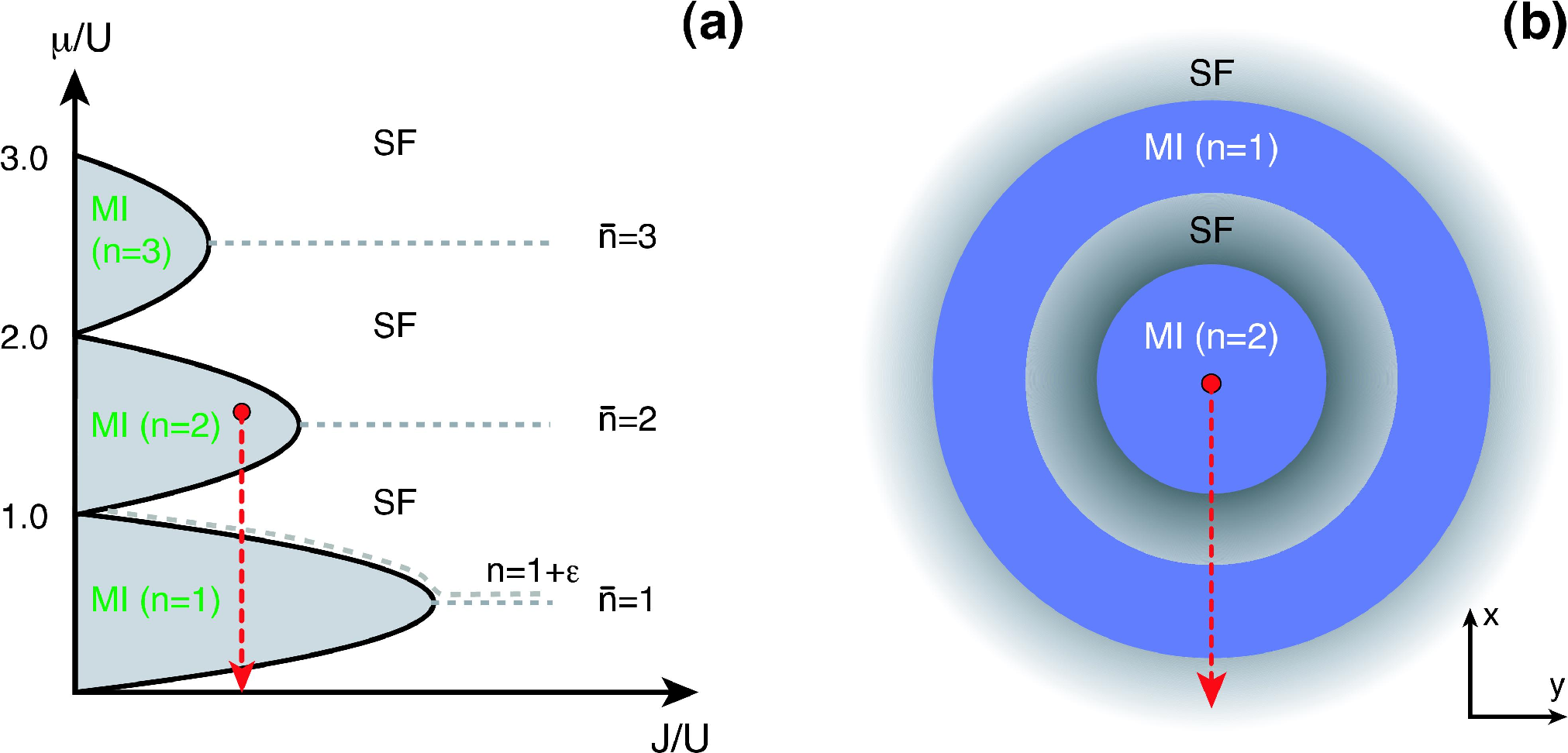
Within a mean-field approximation, the critical value for the transition from a MI to a SF in a three dimensional optical lattice, is given by for and for Fisher et al. 1989; Sheshadri et al. 1993; van Oosten et al. 2001. Here is the number of nearest neighbors and thus is the total bandwidth of the lowest Bloch band, which is the relevant parameter which has to be compared with . Recently, precise Quantum Monte-Carlo simulations by Capogrosso-Sansone et al. 2007 have determined the critical value for the transition in a simple cubic lattice to be at with an accuracy of about %. In one dimension, the SF-MI transition is of the Kosterlitz-Thouless type, with a finite jump of the superfluid density at the transition. Precise values for the critical coupling are available from DMRG calculations, giving Kühner et al. 2000; Kollath et al. 2004 for the transition. For , the BHM is equivalent to a chain of Josephson junctions with coupling energy . The SF-MI transition is then desribed by the -dimensional -model, which gives Hamer and Kogut 1979; Roomany and Wyld 1980.
From Eqs. (38) and (47), the critical value of the dimensionless lattice depth for rather deep lattices is obtained from
| (69) |
Using the experimental parameters nm and nm Greiner et al. 2002a, the precise result for in a simple cubic lattice gives a critical value for the SF-MI transition with . Given that Eq. (38), on which the above estimate for the critical lattice depth is based, is not very precise in this regime, this result is in reasonable agreement with the lattice depth of , where the transition is observed experimentally Greiner et al. 2002a; Gerbier et al. 2005b.
Consider now a filling with which is slightly larger than one. For large the ground state has all the atoms delocalized over the whole lattice and the situation is hardly different from the case of unit filling. Upon lowering , however, the line of constant density remains slightly above the ’Mott-lobe’, and stays in the SF regime down to the lowest (see Fig. 13). For any noninteger filling, therefore, the ground state remains SF as long as the atoms can hop at all. This is a consequence of the fact, that even for there is a small fraction of atoms which remain SF on top of a frozen MI-phase with . Indeed this fraction can still gain kinetic energy by delocalizing over the whole lattice without being blocked by the repulsive interaction because two of those particles will never be at the same place. The same argument applies to holes when is negative. As a result, in the homogeneous system, the quantum phase transition from a SF to a MI only appears if the density is equal to a commensurate, integer value.
In-trap density distribution Fortunately, the situation is much less restrictive in the presence of a harmonic trap. Indeed, within a local density approximation, the inhomogeneous situation in a harmonic trap is described by a spatially varying chemical potential with at the trap center. Assuming e.g. that the chemical potential at trap center falls into the ’Mott-lobe’, one obtains a series of MI domains separated by a SF by moving to the boundary of the trap where vanishes (see Fig. 13b). In this manner, all the different phases which exist for given below are present simultaneously ! The SF phase has a finite compressiblity and a gapless excitation spectrum of the form because there is a finite superfluid density . By contrast, in the MI-phase both and vanish. As predicted by Jaksch et al. 1998, the incompressibility of the MI phase allows to distinguish it from the SF by observing the local density distribution in a trap. Since in the MI, the density stays constant in the Mott phases, even though the external trapping potential is rising. In the limit of the SF regions vanish and one obtains a ’wedding cake’ type density profile, with radii of the different Mott insulating regions, given by DeMarco et al. 2005.
The existence of such wedding-cake like density profiles of a Mott insulator has been supported by Monte-Carlo Kashurnikov et al. 2002; Batrouni et al. 2002; Wessel et al. 2004; Rigol et al. 2006 and DMRG Kollath et al. 2004 calculations in one, two, and three dimensions. Very recently number state resolved, in-trap density profiles have been detected experimentally by Campbell et al. 2006 and Fölling et al. 2006. In the latter case it has been possible to directly observe the wedding cake density profiles and thus confirm the incompressibility of the Mott insulating regions of the atomic gas in the trapping potential. A sharp drop in the radii of the occupied regions has been observed when the crossing the transition point Fölling et al. 2006. It should be noted that the in-trap density profiles can be used as a sensitive thermometer for the strongly interacting quantum gas. For typical experimental parameters, one finds that for temperatures around , the wedding cake profiles become completely washed out Gerbier 2007. Within the strongly interacting regime, the superfluid shells accomodate most of the entropy of the system and can turn already into a normal thermal gas at a lower temperature with the Mott insulating shells still intact Capogrosso-Sansone et al. 2007; Gerbier 2007; Ho and Zhou 2007. In order to reach the lowest temperatures in this regime, it is advantageous to keep the external harmonic confinement as low as possible, or even decrease it during an increase of the lattice depth Gerbier 2007; Ho and Zhou 2007.
Phase coherence across the SF-MI transition The disappearance of superfluidity (or better of BEC) at the SF-MI transition was initially observed experimentally by a time-of-flight method Greiner et al. 2002a. The corresponding series of images is shown in Fig. 14 for different values of , ranging between (a) and (h). One observes a series of interference peaks around the characteristic ’zero-momentum’ peak of a condensate in the absence of an optical lattice. With increasing these peaks become more pronounced. Beyond a critical lattice depth around (e), which agrees very well with the above estimate for the SF-MI transition for one Boson per site, this trend is suddenly reversed, however, and the interference peaks eventually disappear completely. In order to understand why these pictures indeed provide a direct evidence for a SF to MI transition predicted by the Bose-Hubbard model, it is useful to consider the idealized situation of a perfect periodic lattice in the absence of any trapping potential. From Eq. (44) the observed density at position reflects the momentum distribution at . Factoring out the number of lattice sites, it is proportional to the lattice Fourier transform
| (70) |
of the one-particle density matrix at separation . For optical lattice depths below the critical value, the ground state in a 3D situation is a true BEC, where approaches a finite value at large separation. For the MI phase, in turn, decays to zero exponentially. The SF phase of cold atoms in a homogeneous optical lattice is thus characterized by a momentum distribution which exhibits sharp peaks at the reciprocal lattice vectors (defined by times an integer, see e.g. Ashcroft and Mermin 1976) plus a smooth background from the short range correlations. The fact that the peaks in the momentum distribution at initially grow with increasing depth of the lattice potential is a result of the strong decrease in spatial extent of the Wannier function , which entails a corresponding increase in its Fourier transform at higher momenta. In the MI regime, where decays to zero, remnants of the interference peaks still remain (see e.g. Fig. 14f) as long as extends over several lattice spacings, because the series in Eq. (70) adds up constructively at . A more detailed picture for the residual short range coherence features beyond the SF-MI transition is obtained by considering perturbations deep in the Mott insulating regime at . There, vanishes beyond and the momentum distribution is a structureless Gaussian, reflecting the Fourier transform of the Wannier wave function (see Fig. 14h). With increasing tunneling , the Mott state at is modified by a coherent admixture of particle-hole pairs. However due the presence of a gapped excitation spectrum, such particle hole pairs cannot spread out and are rather tightly bound to close distances. They do, however, give rise to a significant degree of short range coherence. Using first order perturbation theory with the tunneling operator as a perturbation on the dominating interaction term, one finds that the amplitude of the coherent particle hole admixtures in a Mott insulating state is proportional to :
| (71) |
Close to the transition point, higher order perturbation theory or a Green function analysis can account for coherence beyond nearest neighbors and the complete liberation of the particle-hole pairs, which eventually leads to the formation of long range coherence in the superfluid regime. The coherent particle hole admixture and its consequence on the short range coherence of the system have been investigated theoretically and experimentally in Gerbier et al. 2005b; Gerbier et al. 2005a; Sengupta et al. 2005.

The SF-MI quantum phase transition therefore shows up directly in the interference pattern. For the homogeneous system it reveals the existence or not of off-diagonal long range order in the one-particle density matrix. The relevant order parameter is the condensate fraction. Of course the actual system is not homogeneous and a numerical computation of the interference pattern is necessary for a quantitative comparison with experiment. This has been done e.g. for the 3D case in Kashurnikov et al. 2002 and for 1D case in Batrouni et al. 2002; Kollath et al. 2004. Due to the finite size and the fact that different MI phases are involved, the pattern evolves continuously from the SF to the MI regime. While the critical values for are different for the MI phases with and which are present in the experiment Greiner et al. 2002a, the transition seen in the time-of-flight images occurs rather rapidly with increasing lattice depth. Indeed, from Eq. (69), the experimental control parameter depends only logarithmically on the relevant parameter of the BHM. The small change from in (e) to in (f) thus covers a range in wider than that, which would be required to distinguish the from the transition. For a quantitative evaluation of the interference patterns, one must also take into account the broadening mechanism during time-of-flight expansion, as discussed in Sec. II.3.
When approaching the SF-MI transition from the superfluid regime, the increasing interactions tend to increase the depletion of the condensate and thereby reduce the long range phase coherent component with increasing Orzel et al. 2001; Hadzibabic et al. 2004; Schori et al. 2004; Xu et al. 2006. For increasing lattice depth, the condensate density as a measure of the long range coherent fraction, then decreases continuously and vanishes at the transition point. The visibility of the interference pattern in general, however, evolves smoothly across the SF-MI transition, due to the presence of a strong short range coherent fraction in the MI just across the transition point (see discussion above). Above the transition point the visibility of the momentum distribution can also show kinks as the lattice depth is increased, which have been attributed to the beginning formation of shell structures in the MI state Gerbier et al. 2005b; Gerbier et al. 2005a; Sengupta et al. 2005.
Excitation spectrum A second signature of the SF-MI transition is the appearance of a finite excitation gap in the Mott insulator. Deep in the MI phase, this gap has size , which is just the increase in energy if an atom tunnels to an already occupied adjacent site (note that is much smaller than the gap for the excitation of the next vibrational state). The existence of a gap has been observed experimentally by applying a potential gradient in the MI Greiner et al. 2002a or by using a modulation spectroscopy method Stöferle et al. 2004 and measuring the resulting excitations. Recent calculations indicate that such measurements simultaneously probe global Iucci et al. 2006; Huber et al. 2007 and local properties of the system. In particular, e.g. a peaked excitation spectrum can also appear in a strongly interacting superfluid regime, where Kollath et al. 2006. A way to probe global features of the many-body excitation spectrum, also close to the transition point, might be achieved by employing Bragg spectroscopy techniques as proposed in van Oosten et al. 2005; Rey et al. 2005; Pupillo et al. 2006.
In the SF regime, there is no excitation gap. Instead, the homogeneous system exhibits a sound like mode with frequency . As shown in the appendix, the associated sound velocity is determined by and thus gives information about the superfluid density . The existence of a sound like excitation even in the presence of an underlying lattice which explicitely breaks translation invariance is a consequence of long range phase coherence in the SF. Its observation would therefore directly probe superfluidity, in contrast to the peaks in the interference pattern, which measure BEC.
Number statistics Associated with the transition from a superfluid to a Mott insulating state is a profound change in the atom number statistics per lattice site. As noted above, in the homogeneous system the ground state in the extreme MI limit () is a product of Fock states with an integer number of particles at each site. At finite hopping , this simple picture breaks down because the atoms have a finite amplitude to be at different sites. The many-body ground state can then no longer be written as a simple product state. In the opposite limit , the ground state is a condensate of zero quasi-momentum Bloch states. In the limit at fixed (not necessarily integer) density , the associated perfect condensate is a product of coherent states on each lattice site
| (72) |
with describing the amplitude and phase of the coherent matter wave field. This corresponds to a Poissonian atom number distribution on each lattice site with average .
A remarkable consequence of the representation (67) is that, at least for integer densities , the many-body ground state may be factorized into a product over single sites
| (73) |
in both limits and . The associated atom number probability distribution is either a pure Fock or a full Poissonian distribution. It is now very plausible to use the factorized form in Eq. (73) as an approximation for arbitrary , taking the coefficients as variational parameters which are determined by minimizing the ground state energy Rokhsar and Kotliar 1991; Sheshadri et al. 1993. As pointed out by Rokhsar and Kotliar 1991, this is effectively a Gutzwiller ansatz for bosons. Beyond being very simple computationally, this ansatz describes the SF to MI transition in a mean-field sense, becoming exact in infinite dimensions. In addition, it provides one with a very intuitive picture of the transition to a MI state, which occurs precisely at the point, where the local number distribution becomes a pure Fock distribution. Indeed, within the Gutzwiller approximation, the expectation value
| (74) |
of the local matter wave field vanishes if and only if the probability for finding different particle numbers at any given site is equal to zero. It is important, however, to emphasize that the Gutzwiller ansatz fails to account for the nontrivial correlations between different sites present at any finite . These correlations imply that the one particle density matrix is different from zero at finite distance , becoming long ranged at the transition to a SF. By contrast, in the Gutzwiller approximation, the one particle density matrix has no spatial dependence at all: it is zero at any in the MI and is completely independent of in the SF. Moreover, in the Gutzwiller approximation, the phase transition is directly reflected in the local number fluctuations, with the variance of vanishing throughout the MI phase. In reality, however, local variables like the on-site number distribution will change in a smooth manner near the transition and the variance of the local particle number will only vanish in the limit .
Crossing the SF-MI transition, therefore, the number statistics evolves rather smoothly from a Poissonian distribution to Fock states on each lattice site. Recent experimental progress has allowed measurements of the number distribution in the optical lattice via microwave spectroscopy exploiting collisional frequency shifts Campbell et al. 2006 or spin changing collisions Gerbier et al. 2006. When crossing the SF-MI transition, Campbell et al. 2006 were able to observe the emergence of a discrete excitation spectrum with Hz resolution. In the second experiment, the change in atom number statistics from Poissonian to Fock states could be revealed Gerbier et al. 2006. Another possibility to observe the number squeezing of the initially Poissonian atom number distribution in the weakly interacting regime due to increasing interatomic interactions has been to use a matter wave beam splitter and observe the timescale of the collapse in the ensuing phase diffusion dynamics Greiner et al. 2002b; Sebby-Strabley et al. 2007; Jo et al. 2007, which is discussed in the following paragraph.
IV.3 Dynamics near quantum phase transitions
One of the major advantages of cold atoms in studying many-body phenomena is the possibility to change the parameters characterizing the relative strength of the kinetic and interaction energy dynamically. This opens the possibility to study the real time dynamics of strongly correlated systems in a controlled manner. As a simple example, we discuss the quench of the system from the superfluid into the Mott insulating regime. This issue has been investigated in an experiment, observing collapses and revivals of the matter wave due to the coherent superposition of states with different atom numbers in the SF Greiner et al. 2002b. In the weakly interacting regime of a BEC in an optical lattice potential, the ground state (67) is a product of coherent states on each lattice site with a Poissonian atom number distribution. If the lattice depth is now suddenly increased to a parameter regime, where the ground state of the system is a Mott insulating state, the initial atom number fluctuations of the coherent state will be frozen out, as the system is not given enough time to redistribute towards the novel many-body ground state. The evolution with time of such a coherent state can be evaluated by taking into account the time evolution of the different Fock states forming the coherent state:
| (75) |
The coherent matter wave field on each lattice site can then simply be evaluated through , which exhibits an intriguing dynamical evolution Yurke and Stoler 1986; Sols 1994; Wright et al. 1996; Imamoglu et al. 1997; Castin and Dalibard 1997; Dunningham et al. 1998. At first, the different phase evolutions of the atom number states lead to a collapse of . However, at integer multiples in time of all phase factors in the above equation re-phase modulo and thus lead to a revival of the initial coherent state . In fact, precise revivals appear as long as the initial state can be written in the factorized form of Eq. (73). Since the time evolution operator factorizes into a product of on-site terms , the time dependence is perfectly periodic with period , where is the value of the on-site repulsion after the quench. Clearly the period is independent of the precise form of the initial number distribution . The collapse time in turn, depends on the variance of the local number distribution. Its measurement thus provides information about how the coherent superposition of different particle numbers in the SF state is eventually destroyed by approaching the MI regime Greiner et al. 2002b.
The collapse and revival of the coherent matter wave field of a BEC is reminiscent to the collapse and revival of the Rabi oscillations in the interaction of a single atom with a single mode electromagnetic field in cavity quantum electrodynamics Rempe et al. 1987; Brune et al. 1996. There, the nonlinear atom-field interaction induces the collapse and revival of the Rabi oscillations whereas here the nonlinearity due to the interactions between the atoms themselves leads to the series of collapse and revivals of the matter wave field. It should be pointed out that such a behavior has also been theoretically predicted to occur for a coherent light field propagating in a nonlinear medium Yurke and Stoler 1986 but to our knowledge has never been observed experimentally. Such a dynamical evolution of the atomic quantum state due to the nonlinear interactions between the particles is also known as quantum phase diffusion and has been detected in Greiner et al. 2002b for low atom numbers on each site. For larger atom numbers, the initial time evolution of the quantum phase diffusion could be recently observed by Jo et al. 2007 in a double well scenario.
The simple single site description is valid only in the limits of a nearly perfect SF in the initial state and of negligible tunneling in the final state. To determine the dynamics in a more general situation, is a complicated non-equilibrium many-body problem. Numerical results for arbitrary values of and have been obtained for the 1D BHM by Kollath et al. 2007, using the time-dependent density matrix renormalization group Schollwöck 2005.
In a related scenario it has be proposed that when jumping from an initial Mott insulating state into the superfluid regime, one should observe oscillations of the superfluid order parameter Altman and Auerbach 2002; Polkovnikov et al. 2002. For large filling factors, oscillating coherence has been observed after a quench from a deep to a shallow lattice by Tuchman et al. 2006. The formation of a superfluid from an initial Mott insulating phase poses a general problem of interest in the context of the dynamics of strongly correlated quantum systems. Both experiment Greiner et al. 2002a and theory Clark and Jaksch 2004 have confirmed that the emergence of coherence in the system can occur rather rapidly on timescales of a few tunneling times . It is an an open question, however, whether off-diagonal long range order in the one-particle density matrix indeed sets in within such a short time and what length scales are relevant over which order has established in order to observe coherence in a time-of-flight picture.
IV.4 Bose-Hubbard model with finite current
The SF-MI transition discussed in IV.2 above is a continuous phase transition in the ground state of a many-body Hamiltonian. The observation from the time-of-flight images, that long range phase coherence is lost beyond a critical value of , provides a signature for the disappearance of BEC. The expected simultaneous loss of superfluidity across this transition may be studied by considering the phase boundary, where stationary states with a finite current loose their stability. Such stationary out-of-equilibrium states may be created experimentally by boosting the condensate to a finite momentum state Fallani et al. 2004, or by inducing a center-of-mass oscillation in the trap Fertig et al. 2005. The question, what happens to the equilibrium SF-MI transition in a situation with a finite current has been addressed by Polkovnikov et al. 2005. For a given number of bosons per site, the kinetic energy term in the BHM (65) gives rise to a Josephson coupling energy due to next neighbor-tunneling which favors a vanishing relative phase between adjacent lattice sites. In the limit , there is non-vanishing matter wave field . In the ground state, all bosons have zero momentum and is uniform. States with a finite current, in turn, are BEC’s in which single particle states with non-zero momentum are macroscopically occupied. To zeroth order in , their energy is the Bloch band energy Eq. (37). The associated current per particle for motion along the -direction has a maximum at . States with a larger momentum are unstable in a linear stability analysis Polkovnikov et al. 2005. This instability was observed experimentally by Fallani et al. 2004. A moving optical lattice is created by two counterpropagating beams at frequencies which differ by a small detuning . Averaged over the optical frequencies, this gives rise to an interference pattern which is a standing wave moving at velocity . Adiabatically switching on such a lattice in an existing BEC then leads to a condensate in a state with quasi-momentum . Its lifetime shows a very rapid decrease for momenta near the critical value .
In the strongly interacting regime near the SF-MI transition, such a single particle picture is no longer valid. At the mean-field level, the problem may be solved by using the field theoretical description of the SF-MI transition. The SF phase is then characterized by a nonzero complex order parameter , whose equilibrium value vanishes like the inverse of the correlation length (this relation holds in the mean-field approximation, which is appropriate for the transition at integer densities in 3D). The stationary solutions of the dimensionless order parameter equation with finite momentum are of the form . Evidently, such solutions exist only if . The critical value of the dimensionless momentum , where current currying states become unstable, thus approaches zero continuously at the SF-MI transition Polkovnikov et al. 2005. In fact, the same argument can be used to discuss the vanishing of the critical current in superconducting wires near , see Tinkham 1996. The complete mean field phase diagram, shown in Fig. 15 interpolates smoothly between the classical instability at and in the limits and respectively. In contrast to the equilibrium transition at which is continuous, the dynamical transition is of first order. Crossing the phase boundary at any nonzero current is therefore connected with an irreversible decay of the current to zero. Experimentally, the decrease of the critical momentum near the SF-MI transition has been observed by Mun et al. 2007. Their results are in good agreement with the phase diagram shown in Fig. 15.

In the mean-field picture, states of a SF with non-zero momentum have an infinite lifetime. More precisely, however, such states can only be metastable, because the ground state of any time-reversal invariant Hamiltonian necessarily has zero current. The crucial requirement for SF in practice, therefore, is that current carrying states have lifetimes which by far exceed experimentally relevant scales. This requires these states to be separated from the state with vanishing current by energy barriers, which are much larger than the thermal or relevant zero point energy 1010 10 This is different from the well known Landau criterion of superfluid flow below a finite critical velocity Pitaevskii and Stringari 2003. Indeed, the existence of phase slips implies that the critical velocity is always zero in a strict sense.. The rate for phase slips near the critical line in Fig. 15 has been calculated by Polkovnikov et al. 2005. It turns out, that the mean-field transition survives fluctuations in 3D, so in principle it is possible to locate the equilibrium SF-MI transition by extrapolating the dynamical transition line to zero momentum. In the experiments of Fertig et al. 2005, the system still showed sharp interference peaks even in the ’overdamped’ regime where the condensate motion was locked by the optical lattice (see Fig. 16). This may be due to localized atoms at the sample edges, which block the dipole oscillation even though the atoms in the center of the trap are still in the SF regime.A theoretical study of the damped oscillations of 1D bosons has been given by Gea-Banacloche et al. 2006.
A different method to drive a SF-MI transition dynamically has been suggested by Eckardt et al. 2005. Instead of a uniformly moving optical lattice, it employs an oscillating linear potential along one of the lattice directions (in a 1D BHM is the dimensionless position operator). For modulation frequencies such that is much larger than the characteristic scales and of the unperturbed BHM, the driven system behaves like the undriven one, however with a renormalized tunneling matrix element , where is the standard Bessel function. Since is unchanged in this limit, the external perturbation completely supresses the tunneling at the zero’s of the Bessel function. Moreover, it allows to invert the sign of to negative values, where e.g. the superfluid phase corresponds to a condensate at finite momentum . It has been shown numerically Eckardt et al. 2005 that by a slow variation of the driving amplitude from zero to (where ) and back to zero allows to adiabatically transform a superfluid into a Mott insulator and then back to a superfluid. In recent experiments by Lignier et al. 2007, the dynamical supression of tunneling with increasing driving has been observed through a measurement of the expansion velocity along the direction of the optical lattice after switching off the axial confinement.

IV.5 Fermions in optical lattices
In this section we would like to focus on fermions in 3D optical lattice potentials and experimental results that have been obtained in these systems (see also Giorgini et al. 2007). Interacting fermions in an periodic potential can be described by the Hubbard hamiltonian. Let us for now restrict the discussion to the case of atoms confined to the lowest energy band and to two possible spin states for the fermionic particles. The single band Hubbard hamiltonian thus reads:
| (76) | |||||
As in the case of bosonic particles, the phase diagram depends strongly on the interaction strength vs. kinetic energy of the atoms in the optical lattices. An important difference between the bosonic and fermionic Hubbard hamiltonian can also be seen in the form of the interaction term, where only two particles of different spin states are allowed to occupy the same lattice site, giving rise to an interaction energy between the atoms.
Filling factor and Fermi surfaces A crucial parameter in the fermionic Hubbard model is the filling factor of the atoms in the lattice. Due to the overall harmonic confinement of the atoms (last term in Eq. (76)), this filling fraction changes over the cloud of trapped atoms. One can however specify an average characteristic filling factor,
| (77) |
with describing the typical delocalization length of the single particle wave-functions in the combined periodic lattice and external harmonic trapping potential Köhl et al. 2005a; Rigol and Muramatsu 2004. The characteristic filling factor can be controlled experimentally, by either increasing the total number of fermionic atoms , by reducing via an increase of the lattice depth or via an increase of the overall harmonic confinement. The latter case however has the disadvantage that a strong harmonic confinement will lead to a decoupling of the independent lattice sites, as the tunnel coupling will not be large enough to overcome the potential energy offset due to the overall harmonic confinement. One is then left with an array of uncoupled, independent harmonic oscillators. The characteristic filling factor of the system can be revealed experimentally by observing the population of the different Bloch states via adiabatic band mapping, introduced in Sec. II.3. By changing the atom number or the lattice depth, Köhl et al. 2005a could thus observe a change from a low filling to a band insulating state, where the single species particles are completely localized to individual lattice sites (see Fig. 17).

Thermometry and pair correlations An important question regarding fermionic quantum gases in optical lattices is the temperature of the many-body system. It has been shown that for non-interacting 50/50 spin mixtures of fermions, the number of doubly occupied spin-states can be used to determine the temperature of the system. For zero temperature and deep optical lattices, one would expect all lattice sites to be occupied by a spin-up and spin-down atom equally. For finite temperatures, however, atoms could be thermally excited to higher lying lattice sites at the border of the system, thus reducing the number of doubly occupied lattice sites. By converting doubly occupied sites into fermionic molecules, it has been possible to determine the number of doubly vs. singly occupied sites and obtain an estimate for the temperature of the spin-mixture Stöferle et al. 2006; Köhl 2006. Another possibility to determine the temperature of the system even for a single species fermionic quantum gas in the lattice has been provided by the use of quantum noise correlations, as introduced in Sec. III . For higher temperatures of the quantum gas, the atoms tend to spread out in the harmonic confinement and thus increase the spatial size of the trapped atom cloud. As the shape of each noise-correlation peak essentially represents the Fourier transform of the in-trap density distribution, but with fixed amplitude of 1 (see Eq. (55)), an increase in the size of the fermionic atom cloud by temperature will lead to a decrease in the observed correlation signal, as has recently been detected in Rom et al. 2006.
When increasing a red-detuned optical lattice on top of a fermionic atom cloud, this usually also leads to an increased overall harmonic confinement of the system. It has been shown that for such a case, the density of states of the system can be significantly modified, thus leading to an adiabatic heating of the fermionic system by up to a factor of two for a strong overall harmonic confinement Köhl 2006. In order to reach low temperatures for the fermionic system, it would thus be advantageous to keep the harmonic confinement as low as possible or even decrease it as the optical lattice depth is increased. Such a configuration is e.g. possible with a blue-detuned optical lattice in conjunction with a red-detuned optical dipole trap.
V COLD GASES IN ONE DIMENSION
In the following it is shown that the confinement of cold atoms in a quantum wire geometry which can be achieved via strong optical lattices Paredes et al. 2004; Kinoshita et al. 2004 provides a means of reaching the strong interaction regime in dilute gases. This opens the possibility to realize both bosonic and fermionic Luttinger liquids and a number of exactly soluble models in many-body physics.
V.1 Scattering and bound states
Consider cold atoms subject to a strong 2D optical lattice in the -plane which confines the motion to the (axial) -direction. In the regime, where the excitation energy for motion in the radial -directions is much larger than the chemical potential, only the lowest transverse eigenmode is accessible. In terms of the oscillator length for the transverse motion, this requires the 1D density to obey . The effective interaction of atoms confined in such a geometry has first been discussed by Olshanii 1998. In the realistic case, where is much larger than the effective range of the atom-atom interaction 1111 11 For a typical frequency kHz, the transverse oscillator length is equal to nm for 87Rb, the two-particle scattering problem at low energies can again be described by a (3D) pseudopotential. However the asymptotic scattering states are now of the form , where is the Gaussian ground state wave function for the transverse motion and the wavevector for motion along the axial direction. Now, away from Feshbach resonances, the 3D scattering length is much smaller than the transverse oscillator length. In this weak confinement limit , the effective 1D interaction is simply obtained by integrating the 3D pseudopotential over the ground state density of the transverse motion. The resulting effective 1D interaction is then of the form with
| (78) |
Trivially, an attractive or repulsive pseudopotential lead to a corresponding sign of the 1D interaction. In order to discuss what happens near Feshbach resonances, where the weak confinement assumption breaks down, we consider the question of possible bound states of two particles in a strong transverse confinement. Starting with an attractive 3D pseudopotential , the effective 1D potential (78) has a bound state with binding energy . With increasing magnitude of , this binding energy increases, finally diverging at a Feshbach resonance. In turn, upon crossing the resonance to the side were , the effective potential (78) becomes repulsive. The bound state, therefore, has disappeared even though there is one in the 3D pseudopotential for . Obviously, this cannot be correct. As pointed out above, the result (78) only applies in the weak confinement limit . In the following we present a treatment of the scattering properties of confined particles for arbitrary values of the ratio . To this end, we will first consider the issue of two-particle bound states with a pseudopotential interaction in quite general terms by mapping the problem to a random walk process. Subsequently, we will derive the low energy scattering amplitudes by analytic continuation.
Confinement induced bound states
Quite generally, two-particle bound states may be determined from the condition of a pole in the exact T-matrix. In the case of a pseudopotential with scattering length , the matrix elements of this equation lead to
| (79) |
in units, where . Here, is the Green function of the free Schrödinger equation and includes both the kinetic energy and the harmonic confining potential. As , the Green function diverges like , thus providing the regularization for the pseudopotential through the second term of Eq. (79). For energies below the bottom of the spectrum of , the resolvent can be written as a time integral. Moreover, by the Feynman-Kac formulation of quantum mechanics, the (imaginary time) propagator can be interpreted as the sum over Brownian motion trajectories from to in time weighted with , where is the external potential in the free Hamiltonian . Similarly, the contribution can be written in terms of the probability density of free Brownian motion with, again, diffusion constant in units where . Taking the limit , Eq. (79) finally leads to the exact equation
| (80) |
for the bound state energies of two particles with a pseudopotential interaction and scattering length . Here is the probability density at the origin of a free random walk after time , starting and ending at , while is the same quantity in the presence of an additional confining potential. Note that in the formulation of Eq. (80), the regularization of the -singularity in is accounted for by the cancellation of the short time divergence due to , because the random walk does not feel the confinement as . For two particles in free space, where at all times, Eq. (80) gives the standard result that a bound state at below the continuum at exists only for , with the standard value . In the presence of an additional confinement however, there is a bound state for arbitrary sign of the scattering length. The quasi-bound state in the continuum at thus becomes a true bound state, i.e. it is shifted upwards by less than the continuum threshold . The physics behind this is the fact that the average time spent near the origin is infinite for the confined random walk. This provides an intuitive understanding for why an infinitesimally small (regularized) delta potential is able to bind a state.
For harmonic confinement, the probability density can be calculated from the determinant for small fluctuations around the trivial Brownian path . Here, obeys the simple by matrix equation Schulman 1981
| (81) |
where is the (diagonal) matrix of the trap frequencies. The fluctuation determinant thus is equal to for the situation with two confining directions and to in the case of a pancake geometry. Since the continua start at and , respectively, we write the bound state energies as or . The dimensionless binding energy in the presence of confinement then follows from the transcendental equation
| (82) |
where is the number of confined directions.

The functions are shown in Fig. 18. For small binding energies , their asymptotic behavior is and with numerical constants and . In the range , where these expansions are quantitatively valid, the resulting bound state energies are
| (83) |
in a 2D pancake geometry or
| (84) |
in a 1D waveguide. These results were obtained, using different methods, by Petrov and Shlyapnikov 2001 and by Bergeman et al. 2003, respectively. With increasing values of the binding energy increases, reaching finite, universal values or precisely at the Feshbach resonance for one or two confined directions. Going beyond the Feshbach resonance, where , the binding energy increases further, finally reaching the standard 3D result in the weak confinement limit . Here the binding is unaffected by the nature of confinement and .
Experimentally, confinement induced bound states have been observed by rf spectroscopy in an array of 1D quantum wires using a mixture of fermionic 40K atoms in their two lowest hyperfine states and Moritz et al. 2005. The different states allow for a finite s-wave scattering length which may be tuned using a Feshbach resonance at G. In the absence of the optical lattice a finite binding energy appears only for magnetic fields below , where . In the situation with a strong transverse confinement, however, there is a nonzero binding energy both below and above . Using Eq. (16) for the magnetic field dependence of the scattering length, its magnitude is in perfect agreement with the result obtained from Eq. (82). In particular, the prediction of a universal value of the binding energy right at the Feshbach resonance has been verified by changing the confinement frequency .
Scattering amplitudes for confined particles
Consider now two-particle scattering in the continuum, i.e. for energies above the transverse ground state energy. Quite generally, the effective 1D scattering problem is described by a unitary S-matrix , with reflection and transmission amplitudes and . They are related to the even and odd scattering phase shifts by the eigenvalues of the S-matrix. In analogy to the 3D case, the corresponding scattering amplitudes are defined as . For the particular case of a delta-function interaction, the odd scattering amplitude and phase shift vanish identically. The relevant dimensionless scattering amplitude is thus simply the standard reflection amplitude. In the low energy limit, a representation analogous to Eq. (4) allows to define a 1D scattering length by 1212 12 As in the 3D case, the scattering length is finite only for potentials decaying faster than . Dipolar interactions are therefore marginal even in one dimension.
| (85) |
with corrections of order because is odd in . The universal limit reflects the fact that finite 1D potentials become impenetrable at zero energy. For a delta-function potential , the low energy form of Eq. (85) holds for arbitrary , with a scattering length , which approaches in the weak confinement limit. More generally, the exact value of for an arbitrary ratio may be determined by using the connection between the bound state energy and a pole at of the 1D scattering amplitude (85) in the upper complex -plane. Using Eq. (84) for the bound state energy in the regime and the fact that must be positive for a bound state, one finds . Since the effective 1D pseudopotential is completely determined by the scattering length , two-particle scattering is described by an interaction of the form
| (86) |
From its derivation, this result appears to be valid only for small and negative, such that the resulting dimensionless binding energy is within the range of validity of Eq. (84). Remarkably, however, the result (86) is exact, as far as scattering of two particles above the continuum is concerned, at arbitrary values of . This is a consequence of the fact that Eq. (86) is the unique pseudopotential consistent with the behavior of up to order . The exact scattering length thus is fixed by the binding energy (84) at small values of . Moreover, the result uniquely extends into the regime where becomes negative, i.e. the pseudopotential ceases to support a bound state. The associated change of sign in at is called a confinement induced resonance Olshanii 1998. It allows to change the sign of the interaction between atoms by purely geometrical means ! As shown by Bergeman et al. 2003, it can be understood as a Feshbach resonance where a bound state in the closed channel drops below the continuum of the ground state. Now, in a 1D waveguide, the separation between energy levels of successive transverse eigenstates with zero angular momentum is exactly , independent of the value of Bergeman et al. 2003. The confinement induced resonance thus appears precisely when the exact bound state energy - which cannot be determined from the pseudopotential (86) unless - reaches . An analogous confinement induced resonance appears in a 2D pancake geometry, see Petrov et al. 2000a.
V.2 Bosonic Luttinger-liquids, Tonks-Girardeau gas
To describe the many-body problem of bosons confined to an effectively 1D situation, the basic microscopic starting point is a model due to Lieb and Liniger 1963
| (87) |
It is based on pairwise interactions with a pseudopotential , as given in Eq. (86). This is a valid description of the actual interatomic potential provided that the two-body scattering amplitude has the low energy form of Eq. (85 for all relevant momenta . In the limit of a single transverse mode, they obey . Remarkably, in this regime, the pseudopotential approximation is always applicable. Indeed, it follows from the leading correction in the low binding energy expansion of the function defined in Eq. (82), that the denominator of the 1D scattering amplitude (85) has the form at low energies with a numerical coefficient . Since in typical situations where , the condition for a negligible cubic term in the scattering amplitude is always obeyed in the regime of a single transverse mode. In this limit, the interaction between cold atoms in a 1D tube is therefore generically described by the integrable Hamiltonian (87). In the homogeneous case, stability requires to be positive 1313 13 For a possible extension to a metastable ’super-Tonks’ regime at see Astrakharchik et al. 2005a, i.e. the 3D scattering length obeys . At a given 1D density the strength of the interactions in Eq. (87) is characterized by a single dimensionless parameter
| (88) |
In marked contrast to the 3D situation, the dimensionless interaction strength scales inversely with the 1D density Petrov et al. 2000b. In one dimension, therefore it is the low density limit where interactions dominate. This rather counterintuitive result can be understood physically by noting that the scattering amplitude Eq. (85) approaches as . Since, at a given interaction strength , the low energy limit is reached at low densities, the atoms in this regime are perfectly reflected by the repulsive potential of the surrounding particles. For , therefore, the system approaches a gas of impenetrable bosons where all the energy is kinetic 1414 14 In fact, it follows from the Lieb-Liniger solution discussed below, that the ratio of the interaction and kinetic energy per particle diverges like for and decreases monotonically to zero as for . In particular, as was shown by Girardeau 1960, at , the hard-core condition of a vanishing wave function whenever two particle coordinates coincide is fulfilled by a wave function
| (89) |
which coincides with the absolute value of the wave function of a non-interacting spinless Fermi gas. Strongly interacting bosons in 1D thus acquire a fermionic character, a fact well known from the exact solution of a hard core Bose or spin system on a 1D lattice in terms of non-interacting fermions by the Jordan-Wigner transformation, see e.g. Wen 2004.
Crossover diagram in a harmonic trap
In the presence of an additional harmonic confinement along the axial direction, the relative interaction strength depends, in addition to the parameter introduced above, also on the ratio between the oscillator length and the magnitude of the 1D scattering length. For a tight radial confinement nm and typical values m for the axial oscillator length, one obtains for 87Rb. This is in fact the interesting regime, since for the typical relative momenta of two particles are so large that the strong interaction limit cannot be reached at all. The conditions for realizing the Tonks-Girardeau (TG) limit in a trap have been discussed by Petrov et al. 2000b using a quantum hydrodynamic description (see also Ho and Ma 1999 and the review by Petrov et al. 2004a on trapped gases in low dimensions). Using Eq. (160) in the appendix, the phase fluctuations in a 1D Bose gas behave like at zero temperature. From the Lieb-Liniger solution discussed below, both the characteristic healing length and the dimensionless so-called Luttinger parameter are monotonically decreasing functions of the interaction strength. In particular, is much larger than one in the limit . In this limit, the 1D Bose gas looses its phase coherence on a scale (defined by ), which exceeds the healing length by an exponentially large factor. The gas behaves like a true condensate as long as its size is smaller than . Applying the Gross-Pitaevskii equation plus the local density approximation, the radius of the associated Thomas-Fermi profile is Petrov et al. 2000b. The condition for the validity of the Thomas-Fermi approximation is thus always obeyed if . In contrast to the analogous situation in 3D, however, the weak coupling regime requires high densities. The local value of the Luttinger parameter at the trap center must thus be large compared to one. This requires or, equivalently, . As a result, the Thomas-Fermi profile becomes invalid if . For particle numbers below , the trapped gas reaches the TG-regime. The density distribution is eventually that of a free Fermi gas, with a chemical potential and a cloud size . The continuous evolution of the density profile and cloud size between the weak coupling and the TG-limit has been discussed by Dunjko et al. 2001.
At finite temperatures, the dominant phase fluctuations are thermal and give rise to a linear increase with distance on a scale , which only depends on the 1D superfluid density 1515 15 To simplify the notation, the dimensionality is not indicated in the superfluid or quasi-condensate densities and .. In a trap of size , these fluctuations are negligible if . Using and the zero temperature result for the Thomas-Fermi radius at , this translates into . In this range, the trapped gas is effectively a true BEC with a Thomas-Fermi density profile and phase coherence extending over the full cloud size. With increasing temperature, phase fluctuations are nongegligible, however density fluctuations become only relevant if exceeds the degeneracy temperature Petrov et al. 2000b. Defining a characteristic temperature below which phase fluctuations are irrelevant over the system size, there is a wide range in which the density profile is still that of a BEC, however phase coherence is lost. The system can be thought of as a collection of independently fluctuating local BEC’s and is called a quasi-condensate Petrov et al. 2000b. At higher temperatures the gas eventually evolves into a non-degenerate regime of a Boltzmann gas. The complete crossover diagram is shown in Fig. 19.
Experimentally, the presence of strong phase fluctuations in a 1D situation already shows up in very elongated 3D condensates which still have a Thomas-Fermi density profile in the radial direction (i.e. such that many transverse modes are involved). In a trap, the strong interaction prevents that local velocity fields due to phase fluctuations show up in the density profile. Switching off the trap, however, the interaction becomes negligible after a certain expansion time and then phase fluctuations are indeed converted into density fluctuations. These have been seen as stripes in absorption images of highly elongated BEC’s by Dettmer et al. 2001. The linear increase of the phase fluctuations at finite temperature leads to an exponential decay of the first order coherence function. The resulting Lorentzian momentum distribution was observed experimentally by Richard et al. 2003 and by Hellweg et al. 2003, using Bragg spectroscopy. This enabled a quantitative measurement of . Moreover, at very low temperatures, no significant density fluctuations were present, thus confirming the quasi-BEC picture in which .

Lieb-Liniger solution
As shown by Lieb and Liniger 1963 the model Eq. (87) can be solved by the Bethe ansatz. The essential physical property which lies behind the possibility of this exact solution is the fact that in one dimension interactions only give rise to scattering but not to diffraction. All eigenstates of the many-body problem in the domain can thus be written as a sum
| (90) |
of plane waves with distinct wave vectors . They are combined with the coordinates in all possible permutations of the . The associated amplitude factorizes into two-particle scattering phase shifts , with the 1D scattering length associated with the pseudopotential . Here, the product runs over all permutations of two wavenumbers which are needed to generate a given permutation of the from the identity. Due to , the two-particle phase shifts are singular as a function of the momenta in the limit of an eventually ideal Bose gas. In the limit , the phase shifts approach for all momenta. Thus is just the parity of the permutation and the Bethe ansatz wave function Eq. (90) is reduced to the free fermion type wave function Eq. (89) of a Tonks-Girardeau gas. For arbitrary coupling, both the ground state energy per particle and the chemical potential are monotonically increasing functions of at fixed density . For weak interactions , the chemical potential follows the behavior expected from a mean field approach, which is valid here for high densities . In the low density regime , in turn, approaches a coupling independent value which is just the Fermi energy associated with . The energy per particle in this regime is of completely kinetic origin, independent of the interaction strength . This remarkable property of the Tonks-Girardeau gas has been observed experimentally by Kinoshita et al. 2004 (see Fig. 20). They have measured the axial expansion energy of an array of 1D Bose gases as a function of the strength of the transverse confinement. Since , the dimensionless coupling is monotonically increasing with at fixed density . In the weak confinement limit, the expansion energy scales linearly with , reflecting the mean field behavior of the average energy per particle. By contrast, for large values of , where becomes shorter than the average interparticle spacing, the energy saturates at a value which is fixed by the density.

The low lying excitations of the Lieb-Liniger model have been obtained exactly by Lieb 1963a. Surprisingly, it turned out that there are two types of excitations, both with a linear spectrum at low momenta. One of them has a Bogoliubov like dispersion, linear at and quadratic at . The crossover from collective to single-particle behavior occurs at a characteristic length , which is related to the chemical potential in the ground state via . In the limit , the crossover length can be expressed in the form . Similar to the situation in three dimensions, the weak coupling regime can therefore be characterized by the fact that the healing length is much larger than the average interparticle spacing , By contrast, for strong coupling , where the chemical potential approaches the Fermi energy of a spinless, non-interacting Fermi gas at density , the healing length is essentially identical with the average interparticle distance. The sound velocity turns out to coincide with the simple thermodynamic formula which is obtained from the quantum hydrodynamic Hamiltonian Eq. (158) under the assumption that the superfluid density at coincides with the full density. The ground state of the Lieb-Liniger gas is in fact fully superfluid at arbitrary values of in the sense of Eq. (156), despite the fact that phase fluctuations destroy plain BEC even at zero temperature. The sound velocity increases monotonically with , approaching the finite value of an ideal Fermi gas in the Tonks-Girardeau limit. The second type of excitations found by Lieb 1963a also has a linear dispersion at small with the same velocity. However, in contrast to the Bogoliubov-like spectrum discussed before, it is restricted to a finite range and terminates with a vanishing group velocity. It turns out, that these excitations are precisely the solitons of the nonlinear Schrödinger equation Ishikawa and Takayama 1980, for a discussion in the cold gas context see Jackson and Kavoulakis 2002.
Momentum distribution in the Luttinger liquid regime
To obtain the momentum distribution of a strongly correlated 1D Bose gas, it is convenient to start from a quantum hydrodynamic description of the one-particle density matrix. At zero temperature, the logarithmic increase of the phase fluctuations with distance (see Eq. (160)), leads to an algebraic decay of at scales beyond the healing length . The associated exponent is rather small in the weak coupling regime and approaches its limiting value in the TG-limit. The resulting momentum distribution thus exhibits a power-law divergence for . At any finite temperature, however, this divergence is cutoff due to thermal phase fluctuations. Indeed, these fluctuations increase linearly with distance on a scale , implying an exponential decay of the one-particle density matrix for . This leads to a rounding of the momentum distribution at small .

Experimentally, the momentum distribution of a Tonks-Girardeau gas has been observed for ultracold atoms in a 2D optical lattice by Paredes et al. 2004. There a weak optical lattice along the one-dimensional quantum gases was applied in order to tune the system into the strongly interacting regime, where is close to one. Indeed, for the low filling factors used in the experiment, there is no Mott insulating phase. The 1D Bose-Hubbard model at describes a bosonic Luttinger liquid with Cazalilla 2004b, where is the effective coupling parameter on a lattice. Increasing the axial lattice depth, this ratio becomes very large, of order . As shown in Fig. 21, the resulting momentum distributions exhibit a power-law decay over a wide momentum range. They are in very good agreement with a fermionization-based calculation of a hard-core Bose gas in a harmonic confinement. The momentum distributions at finite values of have been studied by Quantum Monte Carlo calculations, noting that although the final hardcore limit is only reached for large values of Pollet et al. 2004, the deviations in the momentum distribution compared to fermionized bosons are less than a few percent already for Wessel et al. 2005. In the experiment, a significant deviation from the limiting value of of the exponent in the momentum distribution at small values of is found, which is masked by finite temperature effects and finite size cut-offs. For larger momenta, the momentum distribution of the quantum gas is determined by short-range correlations between the particles, which can increase the coefficient of the power-law decay in the momentum distribution above in the experiment. In fact, it has been shown by Olshanii and Dunjko 2003, that the momentum distribution of a homogeneous 1D Bose gas at large momenta should behave like as long as .
The parameter determines the asymptotic behavior not only of the one-particle density matrix but in fact of all correlation functions. This may be understood from Haldane’s description of 1D Bose liquids 1616 16 In the context of cold gases the notion of a quantum liquid is - of course - purely conventional. These systems are stable only in the gaseous phase, yet may be strongly interacting. in terms of their long wavelength density oscillations Haldane 1981. In its most elementary form, this is just the 1D version of the quantum hydrodynamic Hamiltonian Eq. (158). Introducing a field which is related to the small fluctuations around the average density by , the effective Hamiltonian describing the low lying excitations is of the form
| (91) |
with sound velocity . The low energy physics of a 1D Bose liquid is thus completely determined by the velocity and the dimensionless parameter . In the translation invariant case, is fixed by and the average density. Moreover, for interactions which may be described by a 1D pseudopotential, may be expressed in terms of the microscopic coupling constant by using the Lieb-Liniger solution. The resulting value of decreases monotonically from in the weak interaction, high density limit to in the Tonks-Girardeau limit (see Cazalilla 2004a). The property for repulsive bosons is valid quite generally for interactions which decay faster than such that the 1D scattering length is finite. Formally, the algebraic decay of in a 1D gas at zero temperature is very similar to the situation in 2D at finite temperatures, where exhibits a power law decay with exponent (see Eq. (100)). Apart from the different nature of the phase fluctuations (quantum versus thermal), there is, however, an important difference between both situations. In the 2D case, superfluidity is lost via the BKT-transition once (see Eq. (101)). By contrast, in one dimension, there is no such restriction on the exponent and superfluidity still persists if . The origin of this difference is related to the fact that phase slips in one dimension require a non-zero modulation of the potential, e.g. by a weak optical lattice Büchler et al. 2003. Formally, it is related to a Berry phase term beyond Eq. (91), which confines vortex-antivortex pairs in this case, see Wen 2004.
Two-and three-particle correlations
An intuitive understanding of the evolution from a weakly interacting quasi-condensate to a Tonks-Girardeau gas with increasing values of is provided by considering the pair distribution function . It is defined by the density correlation function and is a measure of the probability to find two particles to be separated by a distance . For an ideal BEC in three dimensions, the pair distribution function is equal to at arbitrary distances. Above , it drops monotonically from to the trivial limit of any homogeneous system on the scale of the thermal wavelength . For cold atoms in 3D, these basic results on bosonic two-particle correlations have been verified experimentally by Öttl et al. 2005 and Schellekens et al. 2005. For the Lieb-Liniger gas, the local value of the pair correlation can be obtained directly from the derivative of the dimensionless ground state energy Gangardt and Shlyapnikov 2003. The exact result for then gives and in the limits and , respectively. For weak coupling, therefore, there is only a small repulsive correlation hole around each particle. By contrast, in the strong coupling limit, the probability to find two bosons at the same point vanishes like . In the Tonks-Girardeau limit, the equivalence of density correlations to that of a free Fermi gas allows to determine the full pair distribution function exactly as . For low densities, therefore, the zero range repulsion strongly suppresses configurations in which two bosons come closer than their mean interparticle distance. Note that the pair correlation exhibits appreciable oscillations with wave vector even though the momentum distribution is completely continuous at . Experimentally, the local value of the pair correlation function has be determined by Kinoshita et al. 2005, using photo-association. As suggested by Gangardt and Shlyapnikov 2003, the rate for stimulated transitions in which two atoms in a continuum state are transferred to a bound molecule is simply reduced by a factor from the corresponding value in 3D, provided the transfer occurs locally on a length scale much less than the transverse oscillator length. The photo-association rate in a one dimensional situation is thus strongly reduced at due to the much smaller probability for two atoms to be at the same point. From measurements of the atom loss after a variable time of photo-association in an array of several thousand 1D traps with particle numbers in the range , Kinoshita et al. 2005 have thus extracted the value of . As shown in Fig. 22 the results are in very good agreement with theory over a wide range of interaction constants up to .

The local value of three-body correlation function has also been calculated by Gangardt and Shlyapnikov 2003. It behaves like and for small or large respectively. The predicted suppression of three-body recombination losses has been observed by Tolra et al. 2004, using the strong confinement in a 2D optical lattice.
In-situ measurements of density fluctuations have been performed by Esteve et al. 2006. They observe a crossover from an effectively high temperature regime at low densities , where the number fluctuations exceed the shot noise level due to bunching in an essentially ideal Bose gas. At high densities, a quasi-condensate regime is reached with , close to the limit of a single transverse mode. There, the number fluctuations are strongly suppressed and may be described by a 1D Bogoliubov description of quasi-condensates Mora and Castin 2003.
Weak optical lattices and coupled 1D gases
The problem of a 1D Bose gas in a weak optical lattice has been discussed by Büchler et al. 2003. Using the extension in 1D of the phase-density representation (159) of the field operator in a quantum hydrodynamic description which accounts for the discrete nature of the particles Haldane 1981, a periodic potential commensurate with the average particle density gives rise to an additional nonlinear term in (91). This is the well known sine-Gordon model Giamarchi 2004, which exhibits a transition at a critical value . For the ground state of the Lieb-Liniger gas remains superfluid in a weak optical lattice. For , in turn, the atoms are locked in an incompressible Mott state even in an arbitrary weak periodic lattice. From the exact Lieb-Liniger result for , the critical value is reached at .
In a configuration using 2D optical lattices, a whole array of typically several thousand parallel 1D gases are generated. For a very large amplitude of the optical lattice , hopping between different 1D gases is negligible and the system decouples into independent 1D tubes. By continuously lowering , however, it is possible to study the crossover from a 1D to a 3D situation. The equilibrium phase diagram of an array of 1D tubes with an adjustable transverse hopping has been studied by Ho et al. 2004. It exhibits a fully phase coherent BEC for sufficiently large values of and the 1D Luttinger parameter . For a detailed discussion of weakly coupled 1D gases see Cazalilla et al. 2006.
V.3 Repulsive and attractive fermions
As mentioned in subsection A, ultracold Fermi gases in a truly 1D regime have been realized using strong optical lattices. In the presence of an additional axial confinement with frequency , the Fermi energy is . The requirement that only the lowest transverse mode is populated therefore requires small particle numbers . Typical temperatures in these gases are around Moritz et al. 2005, which is not small enough, to observe non-trivial many-body effects. We will therefore discuss the basic phenomena which may be studied with ultracold fermions in one dimension only briefly.
In a spin-polarised 1D Fermi gas, only p-wave interactions are possible. As shown by Granger and Blume 2004, the corresponding Feshbach resonances are shifted due to the confinement in a similar way as in (86) above. This was confirmed experimentally by Günter et al. 2005. In the case of two different states, s-wave scattering dominates in the ultracold limit. For repulsive interactions one obtains a fermionic Luttinger liquid, which is basically a two component version of the quantum hydrodynamic Hamiltonian (91). It has a twofold linear excitation spectrum for fluctuations of the total density and the density difference (’spin density’) respectively. Generically, the velocities of ’charge’ and spin excitations are different. This is the most elementary form of ’spin-charge separation’, which has been verified experimentally in semiconductor quantum wires Auslaender et al. 2005. In the context of ultracold Fermi gases in a harmonic trap, spin-charge separation effects show up in collective excitation frequencies Recati et al. 2003 or in the propagation of wavepackets Kollath et al. 2005. A genuine observation of spin-charge separation, however, requires to study single particle correlations and cannot be inferred from collective excitations only.
For attractive interactions, a spin Fermi gas which is described by the basic Hamiltonian Eq. (87) is a so-called Luther-Emery liquid. Its fluctuations in the total density still have a linear spectrum , however there is a finite gap for spin excitations Giamarchi 2004. The origin of this gap is the appearance of bound pairs of fermions with opposite spin. The spectrum for small oscillations of the spin density is similar to that of quasiparticles in the BCS theory. In analogy to Eq. (88) for the bosonic problem, the dimensionless coupling constant is inversely proportional to both the 1D scattering length (now for fermions in different states, note that attractive interactions imply a positive 1D scattering length ) and to the total 1D density . As shown by Gaudin 1967 and Yang 1967, the model is exactly soluble by the Bethe ansatz. For weak coupling, , the spin gap
| (92) |
has a form similar to that in BCS theory, except for an interaction dependent prefactor . Note, however, that the weak coupling regime is reached at high densities , in contrast to 3D, where in the BCS limit. At low densities, where , the spin gap approaches the two-body bound state energy , which was measured by rf-spectroscopy Moritz et al. 2005, as discussed above. In this regime, the tightly bound fermion pairs behave like a hard core Bose gas. The strong coupling BEC limit of attractive fermions in 1D thus appears to be a Tonks-Girardeau gas, very different from the nearly ideal Bose gas expected in a 3D situation (see section VIII). However, in the presence of a harmonic waveguide, the associated transverse oscillator length defines an additional length, not present in a strictly 1D description. As shown in section V.A, the exact solution of the scattering problem for two particles in such a waveguide always exhibits a two-body bound state, whatever the sign and magnitude of the scattering length . Its binding energy right at the confinement induced resonance is equal to . Since in the limit of a singly occupied transverse channel, the two-particle bound state energy is the largest energy scale in the problem beyond this point. In the regime after the confinement induced resonance, where becomes positive, the appropriate degrees of freedom are therefore no longer the single atoms, but instead are strongly bound fermion pairs. An exact solution of the four-body problem in a quasi 1D geometry with tight harmonic confinement shows, that these dimers have a repulsive interaction Mora et al. 2005. Attractive fermions in 1D thus continuously evolve from a fermionic Luther-Emery liquid to a gas of repulsive bosons. As realized by Fuchs et al. 2004 and Tokatly 2004, the 1D BCS-BEC crossover problem can be solved exactly by the Bethe ansatz, connecting the Gaudin-Yang model on the fermionic side with the Lieb-Liniger model on the bosonic side.
The problem of attractive Fermi gases in one dimension at different densities of the two components has recently been solved by Hu et al. 2007b and Orso 2007. The superfluid ground state with equal densities becomes unstable above a critical field . This is the analog of the Clogston-Chandrasekhar limit Clogston 1962; Chandrasekhar 1962, where the paired ground state is destroyed by the paramagnetic, or Pauli, mechanism. In 3D this has been observed by Zwierlein et al. 2006. In contrast to the 3D case, however, the transition is continuous in 1D and the result holds for arbitrary coupling strengths. Moreover, since the gap becomes large at low densities, the SF phase with zero density imbalance appears at the trap edge. The phase in the trap center, in turn, is a partially polarized phase which still has superfluid correlations. As argued by Yang et al. 2001 using Bosonization, this phase exhibits an oscillating superfluid order parameter similar to that predicted by Fulde and Ferrell 1964; Larkin and Ovchinnikov 1965 in a narrow range above the Clogston-Chandrasekhar limit. In contrast to the 3D situation, non-conventional superfluid order is thus expected in a rather wide range of parameters.
VI TWO-DIMENSIONAL BOSE GASES
The two-dimensional Bose gas is a system which presents many interesting features from a many-body physics perspective. The first question that arises concerns the possibility to reach Bose-Einstein condensation in a uniform system. The answer to this question is negative, both for the ideal and the interacting gas. Indeed in reduced dimensionality long range order is destroyed by thermal fluctuations at any finite temperature. However in an interacting 2D gas the destruction of order is only marginal and superfluidity can still occur below a finite critical temperature . Above , the quasi-long range order is destroyed via the mechanism that was elucidated by Berezinskii 1971, and Kosterlitz and Thouless 1973 and which consists in the breaking of pairs of vortices with opposite circulations. As shown by Nelson and Kosterlitz 1977 this scenario implies a jump in the superfluid density1717 17 Note that, unless explicitly indicated, all densities in this section are areal and not volume densities from a finite and universal value to zero, right at . Equivalently, the thermal wavelength obeys . This prediction has been experimentally tested using helium films Bishop and Reppy 1978; Bishop and Reppy 1980.
Quantum atomic gases provide a new system where this concept of a quasi-long range order can be experimentally tested. However the addition of a harmonic potential to confine the gas in the plane changes the problem significantly. For example conventional Bose-Einstein condensation of an ideal gas is possible in a 2D harmonic potential. For an interacting gas, the situation is more involved; a true BEC is still expected at extremely low temperature. At slightly higher temperature phase fluctuations may destabilize it and turn it into a quasi-condensate phase, which is turned into a normal gas above the degeneracy temperature. We review in this section the main features of atomic 2D gases and we discuss the experimental results obtained so far.
We start with an ideal gas of bosons at temperature , confined in a square box of size . Using the Bose-Einstein distribution and assuming a smooth variation of the population of the various energy states, we can take the thermodynamic limit in such a way that the density stays constant. We then find a relation between the density , the thermal wavelength and the chemical potential :
| (93) |
This relation allows one to derive the value of for any value of the degeneracy parameter . It indicates that no condensation takes place in 2D, contrarily to the 3D case. In the latter case the relation between and ceases to admit a solution above the critical value , which is the signature for BEC.
Consider now bosons confined by the potential in the plane. The presence of a trap modifies the density of states and BEC is predicted to occur for an ideal gas when the temperature is below the critical temperature Bagnato and Kleppner 1991:
| (94) |
However it should be pointed out that the condensation remains a very fragile phenomenon in a 2D harmonic potential. To show this point we calculate the spatial density using the local density and semiclassical approximations, which amounts to replacing by in Eq. (93)
| (95) |
Taking to reach the condensation threshold and integrating over , we recover the result (94). But we also note that , which means that the condensation in a 2D harmonic potential occurs only when the 2D spatial density at the center of the trap is infinite. This should be contrasted with the result for a 3D harmonically trapped Bose gas, where condensation occurs at a central density , which is equal (in the semi-classical approximation) to the threshold density in a homogenous system (see e.g. Pitaevskii and Stringari 2003).
VI.1 The uniform Bose gas in two dimensions
We now turn to the more realistic case of a system with repulsive interactions and we consider in this section the case of a uniform gas. We will restrict here to well established results, the main goal being to prepare the discussion of the trapped gas case, that will be addressed in the next section. The first task is to model the atom interaction in a convenient way. As it has been done for a 1D system, it is tempting to use a contact term , which leads to a chemical potential in a mean-field approximation. However two-dimensional scattering has very peculiar properties and we will see that in general it is not possible to describe interactions in 2D by a coupling constant , and that one has to turn to an energy dependent coefficient. We will then discuss the many-body state expected at low temperature, and present briefly the Berezinskii-Kosterlitz-Thouless transition.
We start by some considerations concerning quantum scattering in two dimensions. We consider two particles of mass moving in the plane and we restrict here to low energy motion where the scattering is isotropic. The scattering state can be written Adhikari 1986
| (96) |
where is the incident wave vector and the dimensionless scattering amplitude for the relative energy . At low energy, one gets for the scattering amplitude the following variation
| (97) |
which defines the 2D scattering length . Taking for instance a square well interaction potential of depth and diameter it is equal to , with and . Note that, in contrast to the situation in 3D, where , in 2D tends to 0 when . The total cross-section (dimension of a length), however, tends to infinity.
Since the coupling coefficient is directly related to the scattering amplitude, it appears that 2D systems are peculiar in the sense that the coupling coefficient is intrinsically energy dependent, by contrast to 1D and 3D systems. In addition to the scattering amplitude , one may need the off-shell matrix when addressing many-body problems. It has been calculated for 2D hard disks by Morgan et al. 2002. The extension of the notion of a zero-range interaction potential to the two-dimensional case is discussed by Olshanii and Pricoupenko 2002.
We now turn to a macroscopic assembly of bosonic particles and we first address the situation. The case of a gas of hard disks of diameter and surface density has been studied by Schick 1971. The conclusion is that Bose-Einstein condensation is reached with a large condensate fraction, provided . This constitutes the small parameter of the problem, to be compared with in 3D. The chemical potential is then , indicating that the proper choice for is (within logarithmic accuracy) , where the dimensionless number is equal to the scattering amplitude taken for the energy . Corrections to the result of Schick 1971 for more realistic densities have been calculated by Andersen 2002; Pricoupenko 2004; Pilati et al. 2005.
In the finite temperature case, the impossibility for 2D BEC already mentioned for an ideal gas remains valid for an interacting gas with repulsive interactions. This was anticipated by Peierls 1935 in the general context of long range order in low dimensional systems. It was shown rigorously for interacting bosons by Hohenberg 1967, based on arguments by Bogoliubov 1960. A completely equivalent argument was given for lattice spin systems by Mermin and Wagner 1966. To prove this result one can make a reductio ad absurdum. Suppose that the temperature is small, but finite () and that a condensate is present in the mode , with a density . By the Bogoliubov inequality the number of particles in state satisfies
| (98) |
In the thermodynamic limit, the number of particles in the excited states is
| (99) |
When tends to zero the dominant term in the lower bound given above varies as . In 2D, this leads to a logarithmically diverging contribution of the integral originating from low momenta. This means that the starting hypothesis (existence of a condensate in ) is wrong in 2D.
Even though there is no BEC for a homogeneous, infinite 2D Bose gas, the system at low temperature can be viewed as a quasi-condensate, i.e. a condensate with a fluctuating phase Kagan et al. 1987; Popov 1987. The state of the system is well described by a wave function and the two dimensional character is revealed by the specific statistical behavior of the spatial correlation functions of the phase and the quasi-condensate density . Actually repulsive interactions tend to reduce the density fluctuations and one can in first approximation focus on phase fluctuations only. The energy arising from these phase fluctuations has two contributions. The first one originates from phonon-type excitations, where the phase varies smoothly in space. The second one is due to quantized vortices, i.e. points where the density is zero and around which the phase varies by a multiple of . For our purpose it is sufficient to consider only singly charged vortices, where the phase varies by around the vortex core.

Berezinskii 1971 and Kosterlitz and Thouless 1973 have identified how a phase transition can occur in this system, when the temperature is varied (Fig. 23). At low temperature the gas has a finite superfluid density . The one-body correlation function decays algebraically at large distance:
| (100) |
with . The remarkable fact that there is an exact relation between the coherence properties of the system and the superfluid density is explained in the appendix. Free vortices are absent in this low temperature phase and vortices exist only in the form of bound pairs, formed by two vortices with opposite circulations. At very low temperatures the contribution of these vortex pairs to the correlation function is negligible, and the algebraic decay of is dominated by phonons. When increases, bound vortex pairs lead to a renormalisation of , which remains finite as long as is lower than the critical temperature defined by
| (101) |
Above the decay of is exponential or even Gaussian, once the temperature is large enough that the gas is close to an ideal system. With increasing temperature, therefore, the superfluid density undergoes a jump at the critical point from to 0 Nelson and Kosterlitz 1977. Note that Eq. (101) is actually an implicit equation for the temperature since the relation between the superfluid density and the total density remains to be determined. The physical phenomenon at the origin of the Berezinskii-Kosterlitz-Thouless phase transition is related to the breaking of the pairs of vortices with opposite circulation. For slightly above , free vortices proliferate and form a disordered gas of phase defects, which are responsible for the exponential decay of . For higher temperatures the gas eventually exhibits strong density fluctuations and the notion of vortices becomes irrelevant.
The value given above for the transition temperature can be recovered rather simply by evaluating the likelihood to have a free vortex appearing in a superfluid occupying a disk of radius Kosterlitz and Thouless 1973. One needs to calculate the free energy of this state. The energy corresponds to the kinetic energy of the superfluid; assuming that the vortex is at the center of the disk, the velocity field is , hence , where we set the lower bound of the integral equal to the healing length , since it gives approximately the size of the vortex core. The entropy associated with positioning the vortex core of area in the superfluid disk of area is , hence the expression of the free energy:
| (102) |
For the free energy is large and positive for a large system (), indicating that the appearance of a free vortex is very unlikely. On the opposite for , the large and negative free energy signals the proliferation of free vortices. The critical temperature estimated above from a single vortex picture turns out to coincide with the temperature where pairs of vortices with opposite circulation dissociate. Such pairs have a finite energy even in an infinite system Kosterlitz and Thouless 1973.
The question remains how to relate the various spatial densities appearing in this description, such as the total density , and the superfluid density . In the Coulomb gas analogy where positive and negative charges correspond to clockwise and counterclockwise vortices (see e.g. Minnhagen 1987) these two quantities are related by , where is the dielectric constant of the 2D Coulomb gas. For an extremely dilute Bose gas the relation between and has been addressed by Fisher and Hohenberg 1988. Their treatment is valid in the limit of ultra weak interactions , where is the 2D scattering length. They obtain the result on the low temperature side of the transition point. Using Monte-Carlo calculation, Prokof’ev et al. 2001 have studied the case of weak, but more realistic interactions. Denoting the effective long wavelength interaction constant, they obtain the following result for the total density at the critical point: where the dimensionless number . A typical value for in cold atom experiments is in the range –, which leads to a total phase space density at the critical point in the range –. Prokof’ev et al. 2001 also evaluate the reduction of density fluctuation with respect to the expected result for an ideal gas. They observe that these fluctuations are strongly reduced at the transition point for the domain of coupling parameters relevant for atomic gases. These high precision Monte-Carlo methods also allow one to study the fluctuation region around the transition point Prokof’ev and Svistunov 2005.
The BKT mechanism has been the subject of several studies and confirmations in various branches of condensed matter physics (for a review see Minnhagen 1987). In the context of Bose fluids, Bishop and Reppy 1978 performed an experiment with helium films adsorbed on an oscillating substrate. The change in the moment of inertia of the system gave access to the superfluid fraction and showed a clear evidence for the BKT transition. In an experiment performed with atomic hydrogen adsorbed on superfluid helium, Safonov et al. 1998 observed a rapid variation of the recombination rate of the 2D hydrogen gas when the phase space density was approaching the critical value Eq. (101). However it is still a matter of debate whether one can reach a quantitative agreement between these experimental observations and the theoretical models Kagan et al. 2000; Stoof 1994; Andersen et al. 2002.
VI.2 The trapped Bose gas in 2D
The recent progress concerning the manipulation, cooling and trapping of neutral atomic gases with electromagnetic fields has naturally opened the way to the study of planar Bose gases. In order to prepare 2D atomic gases one freezes the motion along the direction using either light induced forces or magnetic forces. This confining potential has to be strong enough so that all relevant energies for the gas (chemical potential, temperature) are well below the excitation energy from the ground state to the first excited state in . The two other directions are much more weakly confined. The potential in the plane is harmonic in all experiments so far. Here we first review the main experimental schemes that have been implemented. We then discuss the new features that appear because of the harmonic confinement in the plane and we present the current status of experimental investigations concerning the coherence properties of these trapped 2D gases.
Experimental realizations of a 2D gas The conceptually simplest scheme to produce a 2D gas is to use a sheet of light with a red detuning with respect to the atomic resonance. The dipole potential then attracts the atoms towards the locations of high light intensity, and ensures a strong confinement in the direction perpendicular to the light sheet. This technique has been implemented at MIT by Görlitz et al. 2001 for sodium atoms. A 1064 nm laser was focused using cylindrical lenses, and provided a trapping frequency around 1000 Hz along the direction. The red-detuned light sheet also ensured harmonic trapping in the plane, with much smaller frequencies (30 and 10 Hz along the and directions, respectively). An adjustable number of atoms, varying between and , was loaded in the dipole trap starting with a 3D condensate. The measurements were essentially devoted to the size of the atom cloud after free ballistic expansion. For small numbers of atoms (below ) it was observed that the motion was indeed frozen, with a release energy essentially equal to the kinetic energy of the ground state . For larger atom numbers, the interaction energy exceeded and the gas was approaching the 3D Thomas-Fermi limit.
Another way of implementing a 2D trap consists in using an evanescent wave propagating at the surface of a glass prism. In 2004 the group of R. Grimm in Innsbruck loaded such a trap with a condensate of cesium atoms Rychtarik et al. 2004. The light was blue detuned from resonance, so that the atoms levitated above the light sheet, at a distance m from the horizontal glass surface ( Hz). The confinement in the horizontal plane was provided by an additional hollow laser beam, which was blue detuned from the atomic resonance and propagating vertically. This provided an isotropic trapping with a frequency Hz. As in the MIT experiment, a time-of-flight technique revealed that for small atom numbers the vertical expansion energy was approximately equal to , meaning that the motion was frozen. The number of atoms was decreased together with temperature, and a signature of a rapid increase of the spatial density, causing an increase of losses due to 3-body recombination, was observed when the gas approached quantum degeneracy. These data were consistent with the formation of a condensate or a quasi-condensate at the bottom of the trap.
A hybrid trap has been investigated in Oxford, where a blue detuned, single node, Hermite Gaussian laser beam trapped Rb atoms along the direction, whereas the confinement in the plane was provided by a magnetic trap Smith et al. 2005. This allowed to achieve a very large anisotropy factor () between the axis and the transverse plane. Here also the 2D regime was reached for a degenerate gas with atoms.
Trapping potentials that are not based on light beams have also been investigated. One possibility discussed by Hinds et al. 1998 consists in trapping paramagnetic atoms just above the surface of a magnetized material, producing an exponentially decaying field. The advantage of this technique lies in the very large achievable frequency , typically in the MHz range. One drawback is that the optical access in the vicinity of the magnetic material is not as good as with optically generated trapping potentials. Another appealing technique to produce a single 2D sheet of atoms uses the so-called radio-frequency dressed state potentials Zobay and Garraway 2001. The atoms are placed in an inhomogeneous static magnetic field, superimposed with a radio-frequency field, whose frequency is of the order of the energy splitting between two consecutive Zeeman sublevels. The dressed states are the eigenstates of the atomic magnetic moment coupled to the static and radio-frequency fields. Since the magnetic field is not homogeneous, the exact resonance occurs on a 2D surface. There, one dressed state (or possibly several, depending on the atom spin) has an energy minimum, and the atoms prepared in this dressed state can form a 2D gas. This method was implemented experimentally for a thermal gas by Colombe et al. 2004, but no experiment has yet been performed in the degenerate regime.
Finally a 1D optical lattice setup, formed by the superposition of two running laser waves, is a very convenient way to prepare stacks of 2D gases Orzel et al. 2001; Burger et al. 2002; Köhl et al. 2005b; Morsch and Oberthaler 2006; Spielman et al. 2007. The 1D lattice provides a periodic potential along with an oscillation frequency that can easily exceed the typical scale for chemical potential and temperature (a few kHz). The simplest lattice geometry is formed by two counter-propagating laser waves, and it provides the largest for a given laser intensity. One drawback of this geometry is that it provides a small lattice period ( where is the laser wavelength) so that many planes are simultaneously populated. Therefore practical measurements only provide averaged quantities. Such a setup has been successfully used to explore the transition between a superfluid and a Mott insulator in a 2D geometry Köhl et al. 2005b; Spielman et al. 2007. Another interesting geometry consists in forming a lattice with two beams crossing at an angle smaller than 180∘ Hadzibabic et al. 2004. In this case the distance between adjacent planes is adjustable, and each plane can be individually addressable if this distance is large enough Schrader et al. 2004; Stock et al. 2005. Furthermore the tunneling matrix element between planes can be made completely negligible, which is important if one wants to achieve a true 2D geometry and not a modulated 3D situation.
From 3D to 2D scattering In section VI.1 we discussed the properties of a 2D gas consisting of hard disks. Cold atomic gases, however, interact through van der Waals forces, and one has to understand how to switch from the 3D coupling constant to the 2D case. The confining potential along is , and we assume that such that the single atom motion along the direction is frozen into the gaussian ground state.
The scattering amplitude in this regime was calculated by Petrov et al. 2000a, and Petrov and Shlyapnikov 2001. Quite generally, low energy scattering in 2D is described by a scattering amplitude of the form Eq. (97). Since has a pole at , the relation between and the basic scattering length of the 3D pseudopotential may be determined from the bound state energy in a 2D confined geometry. This has been calculated in section V.A for arbitrary values of the ratio between the 3D scattering length and the confinement length . Using Eq. (83) in the limit of small binding energies, the 2D scattering length is related to its 3D counterpart and the confinement scale by
| (103) |
with Petrov and Shlyapnikov 2001. As in 1D, the scattering length for particles in the continuum is determined uniquely by the two-particle binding energy in the limit . The fact that is positive, independent of the sign of , shows that for a 3D interaction described by a pseudo potential, a two-particle bound state exists for an arbitrary sign and strength of the ratio as discussed in section V.A. Note that for realistic parameters nm and of the order of a few nm, the 2D scattering length is incredibly small. This is compensated for by the logarithmic dependence of the scattering amplitude on . Indeed, from Eqs. (97) and (103), the effective low energy scattering amplitude of a strongly confined 2D gas is given by
| (104) |
When the binding along is not very strong, is much larger than so that the logarithm and the imaginary term in (104) are negligible. This weak confinement limit corresponds to the relevant regime for the experiments performed up to now. The resulting scattering amplitude
| (105) |
is independent of energy and the dimensionless coupling parameter is much smaller than one. This implies that the gas is in the weakly interacting regime in the sense that, at the degeneracy point where , the chemical potential is much smaller that the temperature (). An important feature of the dimensional gas is that the criterion for distinguishing the weakly and strongly interacting regime does not depend on density. Indeed the analog of the ratio given in Eq. (88) is simply equal to . In analogy to Eq. (78) in the 1D case, the result (105) can be recovered simply by integrating the 3D pseudopotential over the oscillator ground state. One often refers to a gas in this collisional regime as a quasi-2D system in the sense that it can be considered as a 2D system from the statistical physics point of view, but the dynamics of binary collision remains governed by 3D properties; in particular the 3D scattering length remains a relevant parameter.
More generally, since the relevant energy for relative motion is twice the chemical potential, the momentum in Eq. (104) is just the inverse healing length . At very low energies therefore, the effective interaction in 2D is always repulsive, independent of the sign of the 3D scattering length Petrov and Shlyapnikov 2001. This result, however, is restricted to a regime, where . The logarithmic correction in (104) is therefore significant in the case of a strongly confining potential, when and are comparable. One then recovers a variation for which is formally similar to that of a pure 2D square well (97) with scattering length . This regime could be relevant in a situation where the 3D scattering length is enhanced by a Feshbach resonance Wouters et al. 2003; Rajagopal et al. 2004; Kestner and Duan 2006. If the 3D scattering length is positive, the logarithmic correction in (104) is a mere reduction of the scattering amplitude. On the other hand for a negative , this correction can lead to a strong increase of the amplitude for a particular value of Petrov et al. 2000a, leading to a confinement-induced resonance similar to those that we encountered in the 1D case.
Is there a true condensation in a trapped 2D Bose gas? This question has been strongly debated over the last decade as two opposing lines of reasoning could be proposed. On the one hand we recall that for an ideal gas the presence of a trap modifies the density of states so that Bose-Einstein condensation becomes possible in 2D. One could thus expect that this remains valid in the presence of weak interactions. On the other hand in the presence of repulsive interactions, the extension of the (quasi-)condensate in the trap must increase with the number of atoms . When is large, a local density approximation entails that the correlation function decays algebraically as in (100) over a domain where the density is approximately uniform. This prevents from obtaining long range order except for extremely low temperatures. A related reasoning uses the fact that for the ideal gas, condensation is reached when the spatial density calculated semi-classically becomes infinite (see Eq. (95)), which cannot occur in presence of repulsive interactions. The fragility of the condensation of the ideal Bose gas in 2D is further illustrated by the existence at any temperature of a non-condensed Hartree-Fock solution, for arbitrarily small repulsive interactions Bhaduri et al. 2000. However for very low temperature this solution is not the absolute minimizer of the free energy, as shown using the Hartree-Fock-Bogoliubov method by Fernández and Mullin 2002, Gies and Hutchinson 2004 and Gies et al. 2004.
Currently the converging answer, though not yet fully tested experimentally, is the following: at ultra-low temperature one expects a true BEC, i.e. a system that is phase coherent over its full extension. The ground state energy and density of a 2D Bose gas in the limit can be obtained using the Gross-Pitaevskii equation, as shown rigorously by Lieb et al. 2001 (see also Lee et al. 2002; Kim et al. 2000; Cherny and Shanenko 2001 and Posazhennikova 2006). The cross-over from a three dimensional gas to a two dimensional gas at has been addressed by Tanatar et al. 2002 and by Hechenblaikner et al. 2005.
When the temperature increases one meets the quasi-condensate, superfluid regime, where phase fluctuations due to phonons dominate. The scenario is then very reminiscent of the uniform case and it has been thoroughly analyzed by Petrov et al. 2004a. The function decays algebraically and vortices are found only in the form of bound pairs. Finally at larger temperature these vortex pairs break and the system becomes normal. A BKT transition is still expected in the thermodynamic limit , , constant, but the jump in the total superfluid mass in suppressed because of the inhomogeneity of the atomic density profile Holzmann et al. 2005. Indeed the energy for breaking a vortex pair depends on the local density, and superfluidity will probably be lost gradually from the edges of the quasi-condensate to the center as the temperature increases. Assuming that the atomic distribution is well approximated by the Hartree-Fock solution at the transition point, Holzmann et al. 2005 predict that the BKT transition temperature for a trapped gas is slightly lower than the ideal BEC transition temperature (94), by an amount related to the (small) dimensionless coupling parameter .
We focus for a moment on the quasi-condensate regime. It is described by a macroscopic wave function , and the density and phase fluctuations can be analyzed using a Bogoliubov analysis. We refer the reader to the work of Mora and Castin 2003 and Castin 2004 for a thorough discussion of the extension of Bogoliubov theory to quasi-condensates. As for the uniform gas Prokof’ev et al. 2001, repulsive interactions strongly reduce the density fluctuations for and , so that . For large atom numbers () the equilibrium shape of the gas can be derived using a Thomas-Fermi approximation, as for a true condensate. The kinetic energy plays a negligible role, and the density profile results from the balance between the trapping potential and the repulsive interatomic potential. It varies as an inverted parabola
| (106) |
where the chemical potential and the radius of the clouds are:
| (107) |
with .
The parabolic Thomas-Fermi profile appears on the top of a broader background formed by the atoms out of the (quasi-)condensate. Such a profile has first been experimentally observed by Görlitz et al. 2001 and Rychtarik et al. 2004. A precise measurement of the onset at which a pure thermal distribution turns into a bimodal (Thomas-Fermi + thermal) profile has recently been performed by Krüger et al. 2007. The experiment was performed with a rubidium gas confined in a 1D optical lattice, such that . The phase space density at which bimodality arises was found in good agreement with the prediction of Prokof’ev et al. 2001 for the BKT threshold , which is relevant here if the local density approximation is valid at the center of the trap. At the critical point, the total number of atoms in each plane significantly exceeded the result (94) expected in the ideal case. In this experiment two to three planar gases were actually produced simultaneously, and they could interfere with each other when overlapping during time-of-flight, provided their spatial coherence was large enough. It was observed that the onset of bimodality coincides (within experimental accuracy) with the onset of clearly visible interferences.
It is important to stress that since the expected Thomas-Fermi profile is identical for a true and a quasi-condensate, its observation cannot be used to discriminate between the two situations. The phase fluctuations have been calculated by Petrov and Shlyapnikov 2001 and Petrov et al. 2004a in the regime and (see Eq. (160) in the appendix)
| (108) |
This expression, which is reminiscent of the uniform result (100), is valid for points inside the condensate. The healing length satisfies . Therefore it is only at a temperature much below the degeneracy temperature, such that , that one recovers a quasi uniform phase over the whole sample, hence a true condensate.

Experimental investigations of phase fluctuations A convenient way to access experimentally the phase coherence of quasi-2D gases is the matter-wave heterodyning technique. It consists in studying the statistical properties of the matter wave interference pattern which forms when two independent, parallel 2D Bose gases are released from the trap and overlap (figure 24a). A detailed analysis of these patterns has been given by Polkovnikov et al. 2006 (see section III.C for the 1D case). Assume that the two gases have the same uniform amplitude and fluctuating phases and . The interference signal is recorded by sending an imaging beam along the direction, which integrates the atomic density over a length :
| (109) |
with
| (110) |
The period of the interference pattern is , where is the initial distance between the two planes and the expansion time. We now integrate the coefficient appearing in (109) over a variable length :
| (111) |
and average over many images recorded in the same conditions. Using the fact that the phases and are uncorrelated, we obtain for
| (112) | |||||
where we have assumed that the two gases have the same statistical properties. The long-range physics is then captured in a single parameter, the exponent . It is straightforward to understand the expected values of in some simple cases. In a system with true long-range order, would be constant and the interference fringes would be perfectly straight. In this case , corresponding to no decay of the contrast upon integration. In the low temperature regime, where decays algebraically (see Eq. (100)) the exponent coincides with the exponent which describes the quasi-long range order in . In the high temperature case, where decays exponentially on a length scale much shorter than , the integral in (112) is independent of . In this case , corresponding to adding up local interference fringes with random phases. The BKT mechanism corresponds to a transition between a power law with exponent to an exponential decay of . It should thus manifest itself as a sudden jump of from 0.25 to 0.5 when the temperature varies around .
This method has been implemented at ENS with two rubidium planar gases, forming two parallel, elongated strips (m, m) Hadzibabic et al. 2006 (figure 24b-e). The experimental results confirm the expected behavior, at least qualitatively. At relatively large temperature the fitted exponent is close to . When the temperature decreases a rapid transition occurs and drops to . At the transition the estimated phase space density of the quasi-condensate is . Note that for a quantitative comparison between experiments and theory, one should account for density fluctuations which are likely to play an important point near the transition, in contrast to the situation in superfluid liquid helium. Also the geometry effects in these elongated samples () may be significant.
In addition to the rapid variation of the exponent characterizing the decay of , these experiments also gave evidence for isolated vortices Stock et al. 2005; Hadzibabic et al. 2006 ((figure 24d-e). A vortex appears as a dislocation of the fringes Chevy et al. 2001b; Inouye et al. 2001, and these dislocations indeed proliferate on the high temperature side of the transition. Using a theoretical analysis based on classical field method, Simula and Blakie 2006 obtained phase patterns of quasi-condensates close to the critical temperature that indeed exhibit an isolated, free vortex, in good agreement with experimental observation. The probability for observing a vortex pair in a similar configuration has been calculated by Simula et al. 2005.
The Berezinskii-Kosterlitz-Thouless mechanism has also been recently investigated using a two-dimensional periodic array of Josephson coupled Bose-Einstein condensates Schweikhard et al. 2007. Each tube-like condensate contains a few thousands atoms, and has a length m along the direction. The condensates are localized at the sites of a 2D hexagonal optical lattice of period 4.7m in the plane, and the coupling between adjacent sites can be tuned by varying the optical lattice intensity. The phase properties of the ensemble are probed by ramping down the lattice, and recording the density profile in the plane when the wavefunctions from the various sites overlap. Vortices appear as holes in the atomic density distribution, and the vortex surface density is measured as a function of the Josephson coupling and the temperature . A universal vortex activation curve is obtained as a function of the parameter , showing vortex proliferation for in good agreement with the predictions of the BKT-mechanism.
Breathing mode of a 2D gas In the previous subsection we have been mostly interested in the static properties of 2D Bose gases. Here we point out a remarkable dynamical property of these systems in an isotropic harmonic potential, when the interaction potential between particles is such that . Pitaevskii and Rosch 1997 showed that when the gas is prepared in an arbitrary out-of-equilibrium state, the quantity oscillates at the frequency without any damping, irrespectively of the strength of the interaction. They also proved that this property originates from the presence of a hidden symmetry, described by the two-dimensional Lorentz group SO(2,1). In fact precisely the same symmetry shows up in the case of a unitary gas in 3D, as will be discussed in section VIII.B.
The Dirac distribution in 2D, , belongs to the class of functions satisfying . It makes this SO(2,1) symmetry relevant for trapped neutral atoms at low energies, when the range of interaction is small compared to all other scales. However a true contact interaction is singular in 2D, and leads to logarithmic ultraviolet divergences that are cut off by the finite range of the real interatomic potential. Therefore one cannot hope to observe a fully undamped breathing mode in atomic systems, but rather a very weakly damped dynamics. It was pointed out by Fedichev et al. 2003 that vortex pair nucleation could actually play a role in the residual expected damping of this breathing mode. Note that the difficulties with the contact interaction do not arise at the level of the Gross-Pitaevskii equation, where the same property has been predicted Pitaevskii 1996; Kagan et al. 1996.
A precursor of this long lived breathing mode has been observed in a 3D, quasi cylindrical geometry by Chevy et al. 2001a. The transverse breathing mode of the cylinder was found to oscillate at a frequency very close to with an extremely small damping (quality factor of the mode ). The damping and shift of the oscillation frequency could be calculated theoretically with a good precision by Jackson and Zaremba 2002 (see also Guilleumas and Pitaevskii 2003). In this case part of the damping is due to the nucleation of pairs of phonons propagating along Kagan and Maksimov 2003, a mechanism that is of course absent in a pure 2D geometry. This breathing mode has also been observed in a fast rotating gas by Stock et al. 2004. Its frequency was also , with a small correction due to the non-harmonicity of the trapping potential that was necessary to stabilize the center-of-mass motion of the atom cloud in the fast rotating regime (see section VII.2).
VII BOSE GASES IN FAST ROTATION
The investigation of rotating gases or liquids is a central issue in the study of superfluidity Donnelly 1991. It is relevant for the study of liquid helium, rotating nuclei, neutron stars and pulsars, and for the behavior of superconductors in a magnetic field. During the recent years, several experiments using rotating Bose-Einstein condensates have provided a spectacular illustration of the notion of quantized vortices Matthews et al. 1999; Madison et al. 2000; Abo-Shaeer et al. 2001; Hodby et al. 2001. Depending on the rotation frequency of the gas, a single vortex or several vortices can be observed experimentally. When the number of vortices is large compared to 1, they form a Abrikosov lattice, i.e. a triangular array with a surface density . Since the circulation of the velocity around a single charged vortex is , this ensures that the velocity field of the condensate, when calculated after coarse graining over adjacent vortices, is equal to the orthoradial, rigid body velocity field Feynman 1955.
For a gas confined in a harmonic potential, the fast rotation regime corresponds to stirring frequencies of the order of the trapping frequency in the plane perpendicular to the rotation axis (hereafter denoted ). From a classical point of view the transverse trapping and centrifugal forces then compensate each other, and the motion of the particles in the plane is only driven by Coriolis and interatomic forces. This situation is similar to that of an electron gas in a magnetic field, since Lorentz and Coriolis forces have the same mathematical structure. The single particle energy levels are macroscopically degenerate, as the celebrated Landau levels obtained for the quantum motion of a single charge in a magnetic field. When interactions between atoms are taken into account the fast rotation regime presents a strong analogy with Quantum Hall physics. One can distinguish two limiting cases in this fast rotation regime. Firstly, when the number of vortices inside the fluid remains small compared to the number of atoms , the ground state of the system is still a Bose-Einstein condensate described by a macroscopic wave function . This situation has been referred to as ‘mean field Quantum Hall regime’ Ho 2001; Fischer and Baym 2003. Secondly, when tends to , the number of vortices reaches values comparable to the total number of atoms . The description by a single macroscopic wave function breaks down, and one expects a strongly correlated ground state, such as that of an electron gas in the fractional quantum Hall regime Cooper et al. 2001.
In this section we start by setting the Lowest Landau Level (LLL) framework for the discussion of the fast rotation regime, and discuss the main properties of a fast rotating condensate, when the mean-field description remains valid. We then present recent experimental results where the LLL regime has indeed been reached. Finally we review some theoretical proposals to reach beyond mean field physics, that present a close analogy with the physics of the fractional quantum Hall effect. We do not discuss here the physics of slowly rotating system, where one or a few vortices are involved. We refer the interested reader to the review article of Fetter and Svidzinsky 2001 and to the recent book by Aftalion 2006. Note that a rigorous derivation of the Gross-Pitaevskii energy functional in the slowly rotating case has been given by Lieb and Seiringer 2006.
VII.1 The Lowest Landau Level formalism
The Landau Levels.
We consider first a single particle confined in a two-dimensional isotropic harmonic potential of frequency in the plane. We are interested here in the energy level structure in the frame rotating at angular frequency () around the axis, perpendicular to the plane. The hamiltonian of the particle is
| (113) |
with , ; is the component of the angular momentum. Eq. (113) is formally identical to the hamiltonian of a particle of unit charge placed in a uniform magnetic field , and confined in a potential with a spring constant . A common eigenbasis of and is the set of (not normalized) Hermite functions
| (114) |
where and are non-negative integers and . The eigenvalues are for and
| (115) |
for . For , these energy levels group in series of states with a given , corresponding to the well known, infinitely degenerate, Landau levels. For slightly smaller than , this structure in terms of Landau levels labeled by the index remains relevant, as shown in Fig. 25. Two adjacent Landau levels are separated by , whereas the distance between two adjacent states in a given Landau level is . It is clear from these considerations that the rotation frequency must be chosen smaller than the trapping frequency in the plane. Otherwise the single particle spectrum (115) is not bounded from below. Physically, this corresponds to the requirement that the expelling centrifugal force must not exceed the trapping force in the plane .

We now consider an assembly of cold identical bosons rotating at a frequency close to . Since the effective trapping potential in (113) becomes weaker as increases, we expect that as the equilibrium size of the atom cloud increases indefinitely, and the interaction energy and the chemical potential tend to zero. We define the Lowest Landau Level regime as the situation where , so that the state of the system can be accurately described in terms of Hermite functions with only. Each basis function is proportional to and takes significant values on a ring centered on with an average radius and a width . Any function of the LLL is a linear combination of the ’s and can be cast in the form:
| (116) |
where and is a polynomial (or an analytic function) of . When is a polynomial of degree , an alternative form of is
| (117) |
where the () are the complex zeroes of . Each is the position of a single-charged, positive vortex, since the phase of changes by along a closed contour encircling . Therefore in the LLL, there is a one-to-one correspondence between atom and vortex distributions, contrarily to what happens for slower rotation frequencies. This has interesting consequences on the hydrodynamics of the gas, which cannot be described by conventional Bernoulli and continuity equations Bourne et al. 2006.
Equilibrium shape of a fast rotating BEC.
We now address the question of the distribution of particles and vortices in the case of fast rotation, assuming for the moment that a mean field description is valid. We suppose that the motion along the rotation axis is frozen in a way similar to what we considered in the previous section devoted to static 2D gases.
Consider first the case of an ideal gas. At zero temperature all atoms accumulate in the ground state. At low but finite temperature () the occupied states belong to the LLL. The gas can be described at any time by a Hartree wave function of the type (116), where the coefficients of the polynomial are random independent variables. This fast rotating ideal gas can thus be viewed as a physical realization of a random polynomial Castin et al. 2006. A measurement of the density distribution of the gas will reveal the presence of the vortices, i.e. the roots of . Although the gas is ideal, one can show that the positions of the vortices are correlated and exhibit a strong anti-bunching phenomenon (see Castin et al. 2006 and refs. in).
The case of a fast rotating condensate with repulsive interactions has been analyzed by several authors Ho 2001; Watanabe et al. 2004; Aftalion et al. 2005; Cooper et al. 2004 and we will now review the main results. In all this section we will assume that the pair-wise interaction between atoms and can be described by the contact term . We will furthermore assume that the 3D scattering length is much smaller that the extension of the ground state of the motion along , so that , with (see Eq. (105)). Note that the restriction of the contact interaction to the LLL subspace is a regular operator: it does not lead to the same mathematical difficulties as the ones encountered by considering the contact interaction in the whole Hilbert space of 2D wave functions. In fact, quite generally, interactions in the LLL are described by the Haldane pseudopotentials Haldane. 1983. For a pseudopotential with scattering length , the resulting 2D contact interaction has for and zero otherwise. In the fermionic case, where only odd values of are allowed, the analog of this interaction is a hard core model, where only for . The fact that the Laughlin states, to be discussed in subsection C below, are exact eigenstates for such pseudopotentials has been realized by Trugman and Kivelson 1985.

We start with a gas rotating exactly at the trap frequency (), with an infinite number of particles, but a finite spatial density. In this case the numerical minimization of the Gross-Pitaevskii energy functional indicates that the vortices form an infinite regular triangular lattice. We turn now to a gas with a finite number of particles, rotating at a frequency slightly below . The initial treatment of Ho 2001 assumed an infinite, regular triangular vortex lattice also in this case. The total energy of the system was minimized by varying the spacing of the vortex lattice. When injected in (117) this led to the prediction of a Gaussian atom distribution after coarse-graining over the vortex lattice spacing. A more detailed analysis has recently been performed, where the position of each vortex is taken as a variational parameter Watanabe et al. 2004; Aftalion et al. 2005; Cooper et al. 2004 (see also the work of Anglin 2002 and Sheehy and Radzihovsky 2004a; Sheehy and Radzihovsky 2004b for the case of a slower rotation). One spans in this way the whole LLL subspace. These studies have shown that the vortex distribution that minimizes the total energy is nearly regular with the density close to the center of the condensate, but it is strongly deformed on the edges, with a rarefaction of vortices. For large atom numbers, the predicted coarse-grained density distribution is not gaussian as for a uniform vortex lattice, but it approaches a Thomas-Fermi distribution similar to (106), for the effective trapping potential . This Thomas-Fermi prediction is in good agreement with the results obtained in the experiments described later in this section. The cloud radius is
| (118) |
and diverges for , as expected from the compensation of the trapping force by the centrifugal one. The dimensionless coefficient is the Abrikosov parameter Kleiner et al. 1964 for a triangular lattice. It expresses the fact that due to the restriction to the LLL and to the presence of vortices, the energy and the size of the condensate are actually slightly larger than what one would expect for a static trap with spring constant and a smooth equilibrium distribution. The chemical potential is
so that the condition for the validity of the LLL approach reads . It is also instructive to calculate the number of ‘visible’ vortices, i.e. those which sit in the disk of area . Using so that , we get
As we will see further, the mean field approach is valid only if so that the validity domain of the mean field LLL approach corresponds to the interval:
| (119) |
Note that the total number of vortices, including those sitting outside the Thomas-Fermi radius, can be shown to be infinite for the wave function that minimizes the energy in the LLL subspace Aftalion et al. 2006.
It is interesting to compare the behavior of a fast rotating BEC with that of a fast rotating bucket of superfluid liquid helium, or a type II superconductor in a large magnetic field Fischer and Baym 2003. In the latter cases, the size of the sample is constant and the vortex density increases as the rotation frequency (or the magnetic field) increases. Since the size of a vortex core depends only on the spatial density of the fluid ( the healing length ), it stays constant as increases and one reaches eventually a point where the cores of adjacent vortices overlap. This corresponds to a loss of superfluidity or superconductivity. For superfluid liquid helium, the rotation frequency where this phenomenon should happen is out of reach for realistic experiments. For superconductors on the contrary, the critical field where the superconductivity is lost is a relevant experimental parameter. For fast rotating, harmonically trapped gases, the scenario is very different: (i) the vortex density saturates to a constant value when approaches ; (ii) the size of the vortex core for a wave function of the type (117) is no longer dictated by interactions that would lead to as for an incompressible fluid, but it is on the order of the vortex spacing . Therefore the fractional area occupied by vortices tends to a finite value, as the trapped BEC rotates faster and faster. The cross-over between the standard to the LLL regime is studied in detail by Baym and Pethick 2003 and Cozzini et al. 2006.
VII.2 Experiments with fast rotating gases
The most intuitive way to rotate a trapped atomic gas is to superpose a rotating anisotropic potential to the axi-symmetric trapping potential . The stirring anisotropy can be written where the coordinates are deduced from the static ones by a rotation of angle . The dimensionless parameter characterizes the strength of the stirring potential with respect to the trapping one. In practice, because of experimental limitations, has to be on the order of at least a few percents. Indeed it must overcome by a significant factor the residual static anisotropy of the trapping potential, that is typically in the range Guéry-Odelin 2000.
The stirring potential can be created by a modulated laser beam Madison et al. 2000; Abo-Shaeer et al. 2001 or by a rotating magnetic field Hodby et al. 2001; Haljan et al. 2001. The stirring method has been successfully used to nucleate single vortices as well as large vortex arrays in rotating BECs. However it is not fully appropriate to approach the fast rotating regime of a harmonically trapped gas. Indeed the center-of-mass motion of the atom cloud is dynamically unstable when the rotation frequency is set in the interval Rosenbusch et al. 2002. A precise description of the rotating system at the edge of the instability region has been given by Sinha and Shlyapnikov 2005 (see also Fetter 2007) who showed that the gas forms in this case a novel elongated quantum fluid, with a roton-maxon excitation spectrum. Excitation modes with a zero energy appear above a critical interaction strength, leading to the creation of rows of vortices.
A possible way to circumvent the center-of-mass expulsion occurring at consists in adding a extra trapping potential, that provides a stronger than quadratic confinement. This method has been explored experimentally by Bretin et al. 2004. In this experiment the dipole potential created by a strongly focused laser beam provided a quartic confinement, in addition to the usual quadratic one. It was then possible to explore the critical region and to approach the LLL regime . A striking observation was a strong decrease of the visibility of the vortex pattern in this region. Its origin is not fully understood yet, but it may be related to the fact that the rotating gas was not in the 2D regime. The shape of the rotating cloud was close to spherical, and the vortex lines may have undergone a strong bending with respect to the trap axis, which made them hardly visible in the imaging process. This explanation is favored by the theoretical study by Aftalion and Danaila 2004: when looking for the ground state of the system using imaginary time evolution of the Gross-Pitaevskii equation, it was found that much longer times were required for to reach a well-ordered vortex lattice.
Note that the addition of a quartic potential brings some interesting and novel aspects to the vortex dynamics in the trap, with the possibility to nucleate ‘giant’ vortices. This was initially explored by Fetter 2001, Lundh 2002, Kasamatsu et al. 2002. The mean-field description of the dynamics of a BEC in non harmonic potentials has been recently the subject of an important theoretical activity, and we refer the interested reader to the work of Cozzini et al. 2006 and references in.

Another successful method to reach the fast rotation regime is the evaporative spinup technique, developed by Engels et al. 2002. The cloud is first set in rotation at a frequency notably below using a magnetic stirrer, that is subsequently switched off. Then a nearly one dimensional radio-frequency evaporation along the axis of rotation cools the cloud. Simultaneously the rotation speed of the gas increases since the evaporated atoms carry less angular momentum than average. With this tool the Boulder group has succeeded in producing a gas rotating at with a purely harmonic confinement. Thanks to the centrifugal deformation, the radius of the gas in the plane increases whereas the thickness along shrinks to the size of the ground state , setting the gas well inside the 2D regime. As the total volume of the gas increases, interactions are reduced: the chemical potential Hz drops below the splitting between two Landau levels (17 Hz), and the LLL regime is reached Schweikhard et al. 2004. With this setup, the Boulder group has been able to test the prediction that the fractional core area of the vortices saturates to a value of the order of 0.2 Coddington et al. 2004; Schweikhard et al. 2004, as predicted theoretically Baym 2003 (figure 27). In addition the expected distortion of the vortex lattice with respect to an ideal triangular array could be detected experimentally on the edge of the rotating condensate Coddington et al. 2004. Following a suggestion by Anglin and Crescimanno 2002, another interesting investigation performed on this system dealt with the Tkachenko oscillations Tkachenko 1966 (for a review see Sonin 1987), i.e. the long-wavelength transverse excitations of the vortex lattice Coddington et al. 2003. The Tkachenko waves could be directly imaged and their frequency could be measured with a good precision. The theoretical analysis of these oscillations has recently been performed within the mean-field approximation by several authors (Baym 2003; Baym 2004, Gifford and Baym 2004, Choi et al. 2003, Baksmaty et al. 2004, Woo et al. 2004, Mizushima et al. 2004, Sonin 2005a; Sonin 2005b, Cozzini et al. 2004 and Chevy 2006).
Fast rotation of a BEC can also be achieved by stirring the gas with a potential that is more elaborate than a quadratic one. One can use in particular a rotating optical lattice that creates a rotating, spatially periodic pattern on the gas. This has been explored recently by Tung et al. 2006, who superimposed to a rotating BEC a set of columnar pinning sites created by a two-dimensional, co-rotating optical lattice. For a sufficiently large laser intensity the optical lattice can impose its structure to the vortex lattice; Tung et al. 2006 studied in particular the transition from the usual triangular Abrikosov lattice to a square configuration imposed by light. Theoretical investigations of this problem were carried out by Pu et al. 2005 and Reijnders and Duine 2004; Reijnders and Duine 2005, who found that a rich variety of structural phases can emerge in this geometry, from the competition between vortex-vortex and vortex-optical lattice interactions.
VII.3 Beyond the mean field regime
In the mean-field description of a fast rotating gas, the macroscopic wave function is a solution of the non-linear Gross-Pitaesvkii equation and corresponds to a vortex lattice. The radius of the atom cloud, given in (118), is a measure of the number of single particle LLL states that have a significant population. Recalling that is maximum for a radius , we find
| (120) |
The filling factor gives the average number of particles in each occupied single particle state. When on expects the mean field treatment to be valid, and is equal to the number of visible vortices sitting in the atom disk. On the opposite when tends to , becomes on the order of unity or below, the number of vortices exceeds the number of atoms , and one has to turn to a full many-body treatment of the problem. This breakdown of mean-field approximation occurs when
| (121) |
The analysis of this ultra-fast rotating regime presents strong analogies with the studies of the fractional quantum Hall effect (FQH). In the latter case one is interested in the correlated state of a 2D electron gas with Coulomb interaction when it is placed in a strong magnetic field. In both cases the states of interest are restricted to the LLL and one looks for specific filling factors where ground states with specific properties can emerge. Note, that for bosons the filling factor can be arbitrarily large within the LLL, while for fermions it is restricted to . One remarkable feature is incompressibility, meaning that the ground state is separated from all excited states by a ‘macroscopic’ energy gap scaling as . Moreover it leads to the appearance of edge states near the boundary of the system, similar to the wedding-cake structure of the Mott-insulating state of the Bose-Hubbard model. These edge states are crucial for understanding the quantization of the Hall conductance, see MacDonald 1994 and - on a more mathematical level - Fröhlich and Studer 1993.
Numerical studies.
So far the ultra-fast rotation regime has not been reached experimentally. Even for the fastest rotations realized in the laboratory, the filling factor is (, ), well inside the mean field regime. Therefore the results obtained so far originate from an exact numerical diagonalization of the many-body hamiltonian and from the connection with know features of the fermionic FQH.
Most studies are performed considering states with a given total angular momentum , so that the problem essentially consists in finding the eigenstates of the interaction energy
| (122) |
All states considered hereafter belong to the LLL subspace, so their functional form in the plane is
| (123) |
where , , and where is a symmetric polynomial. The motion is expected to be ‘frozen’ to its ground state and it is not explicitly written in what follows. If one is interested only in the bulk properties of the vortex liquid state, it is convenient to replace the inhomogeneous disk geometry of a real experimental setup by a compact, homogeneous geometry. Both torus Cooper et al. 2001 and spherical Regnault and Jolicoeur 2003; Nakajima and Ueda 2003 manifolds have been considered. The LLL is then a space of finite dimension , proportional to the area of the torus or the sphere: . This allows to define in a non ambiguous way the filling factor () even for values on the order of 1 or below, where the notion of visible vortices becomes dubious.
Melting of the vortex lattice.
When increasing the rotation speed of the gas, the first expected deviation from the mean-field regime is the quantum melting of the vortex lattice. This has been observed by Cooper et al. 2001 in exact numerical calculations for filling factors to . This value can be recovered by calculating the quantum fluctuations of vortex positions and applying the Lindemann criterion , where is the vortex spacing Sinova et al. 2002. For smaller than the melting threshold, one meets for the ground state of the many-body system a series of strongly correlated ground states that we now briefly discuss.
The Laughlin state and its daughter states.
Since increasing the angular momentum spreads out the atoms in space, one expects the interaction energy of the ground state for a given to decrease as increases (see e.g. Jackson and Kavoulakis 2000). This decrease stops when one reaches the celebrated Laughlin wave function, adapted here for bosonic particles:
| (124) |
Indeed since the probability to get two particles at the same point vanishes, this state has the remarkable property to be an eigenstate of the contact interaction potential with eigenvalue 0 Trugman and Kivelson 1985. Increasing beyond this point cannot reduce further . The total angular momentum of this state is equal to the degree of each term of the polynomial and this state expands over all LLL single particle wavefunctions from to , i.e. a filling factor . The Laughlin state is incompressible and the gap to the first excited state is Regnault and Jolicoeur 2003; Regnault and Jolicoeur 2004. The Laughlin state is characterized by a quasi-uniform density of particles over the circle of radius . The two-body correlation function for this state shows a strong anti-bunching . This correlation function has been calculated numerically for a number of bosons up to 8 by Barberán et al. 2006.
For , any state , where is a arbitrary symmetric polynomial, is a ground state of the system with interaction energy 0. Depending on the total degree of , the physical interpretation of the state can be: (i) for , edge excitations of the Laughlin state Cazalilla 2003; Cazalilla et al. 2005, (ii) for , quasi-holes at a given point are obtained by taking Paredes et al. 2001; Paredes et al. 2002, (iii) for , Laughlin-type wave functions with smaller filling factors, by replacing the exponent by in (124).
The composite Fermion sequence.
For filling factors between the melting point and the Laughlin state , it is not possible to give an exact analytical expression of the ground state at any given . One finds however a strong overlap between the numerically determined ground states and some relevant states for the physics of electronic FQH. An example is the composite fermion sequence which presents strong analogies with the Jain principal sequence for fermions Jain 1989. A first evidence for this sequence was found by Cooper and Wilkin 1999, and it has been studied in detail by Regnault and Jolicoeur 2003; Regnault and Jolicoeur 2004. The physics at the origin of the states of this sequence is reminiscent of that explored in the section on 1D gases, where the problem of bosonic particles with repulsive interaction is mapped onto the properties of an assembly of non-interacting fermionic particles. Here one considers that the gas is formed with fermionic composite entities, each resulting from the attachment of a fermionic particle with a vortex carrying one unit of statistical flux. These composite fermions can be viewed as independent particles which occupy various Landau levels. When they occupy exactly Landau levels they form an incompressible state. This occurs when the filling fraction in the initial state is . From a more quantitative point of view, the composite fermion ansatz corresponds to a wave function of the type:
| (125) |
describe the projector onto the LLL subspace (for its precise definition see e.g. Chang et al. 2004). The first term in the bracket is a Slater determinant giving the state of fictitious fermions filling exactly Landau levels. The second term involving products of (Jastrow factor) corresponds to the attachment of a vortex to each fermion. Since both terms in the bracket are antisymmetric in the exchange of two particles, their product is a symmetric wave function, suitable for the description of our identical bosons. Numerical evidence for such states was obtained for and by Regnault and Jolicoeur 2003; Regnault and Jolicoeur 2004 and Chang et al. 2004. The surface waves of the vortex liquids whose wave functions can be described by the composite fermion ansatz have been studied by Cazalilla 2003, Regnault and Jolicoeur 2004 and Cazalilla et al. 2005.
The Read-Moore state and the Read-Rezayi series.
For the filling factor yet another type of approximate ground state have been identified Cooper et al. 2001, the Moore-Read state, or Pfaffian. Assuming that is even the expression of this state is
| (126) |
where indicates symmetrization over all indices. The total degree of each term of this polynomial is and the state expands over single particle LLL wavefunctions from up to , corresponding to a filling factor . As for the ground state is incompressible with a gap Chang et al. 2004. It is noteworthy that for this state, the probability is zero to have three particle at the same location in space.
For even larger filling factors ( between 1 and 10) an analysis performed in a torus geometry suggested that the system has incompressible ground states belonging to a family containing clusters of particles Cooper et al. 2001 and corresponding to integer or half integer filling factors. This so-called Read-Rezayi series Read and Rezayi 1999 is constructed by taking symmetrized products of Laughlin states of the type (assuming that is a multiple of ). The Laughlin and the Moore-Read states corresponds to and , respectively. The filling factor associated to these states is and the total angular momentum is . Further calculations performed in the spherical geometry could not draw any conclusion concerning the survival of the incompressibility of such states at the thermodynamic limit Regnault and Jolicoeur 2004.
Possible detection schemes for fractional quantum Hall effects.
We now review some possible ways for observing experimentally effects related to fractional quantum Hall physics. We first note that it is unlikely that condensed-matter-type techniques, based on transport properties with specific conductance plateaus can be implemented with rotating atomic gases, at least in the near future. We also point out that the condition (121) giving the threshold for the observation of mean-field effects imposes de facto to work with very small atomic samples. Consider for example a purely harmonic trap. Due to residual trap imperfections it is seems unlikely that one can achieve rotation frequencies larger than (rotation frequencies have been achieved by Schweikhard et al. 2004). Taking , this sets an upper bound of on the atom number. Working with such small atom numbers is not untractable, but it immediately makes this type of experiment quite challenging from a technical point of view.
A first possible experimental signature of the Laughlin and Read-more states could lie in the fact that 3 particles can never sit at the same location in space for these wave functions. As 3-body recombination is often the main source of atom losses one can expect that the achievement of these states could be revealed by a spectacular increase of the lifetime of the gas, as it has been the case for 1D physics Tolra et al. 2004.
We now turn to more quantitative studies of these incompressible states. A ‘simple’ experimental evidence for a state such as the Laughlin wave function could come from its specific density profile, which is uniform over a disk of radius , and zero elsewhere. This flat profile with density is notably different from the parabolic density profile expected in the mean-field regime, and its observation would constitute a clear signature of a beyond mean-field effect. Usually one does not measure directly the in-trap density profile, because the relevant distances are on the order of a few micrometers only, which is too small to be detected with a good accuracy by optical means. The standard procedure to circumvent this problem is to use a time-of-flight technique, where the potential confining the atoms is suddenly switched off so that the atoms fly away ballistically during an adjustable time before being detected. For an arbitrary initial state the functional form of the density distribution is modified during the time-of-flight. For an LLL wavefunction this modification is a mere scaling, at least when interactions between atoms are negligible during the time-of-flight Read and Cooper 2003. In particular the disk shape structure associated with the Laughlin state should remain invariant in ballistic expansion.
If the number of atoms is larger than the one required to form a Laughlin wave function at the particular frequency that is used, one expects a ‘wedding cake’ structure for the atomic density Cooper et al. 2005. This result is obtained within a local density approximation and is very reminiscent of the structure appearing in an atom Mott insulator confined in a harmonic trap. At the center of the trap where the density is the largest, the atoms may form an incompressible fluid corresponding for example to the filling factor , which is one of the composite fermion states identified above. The atomic density is then expected to be constant and equal to over a central disk of radius . For the gas switches abruptly (over a distance ) to the Laughlin state with filling factor and the density drops to the value . It then stays constant over a ring of outer radius () and for the density drops to zero. The values of and can be obtained from a simple energy minimization Cooper et al. 2005. For larger atom numbers, several plateaus, with decreasing densities corresponding to the various filling factors of the incompressible states, are expected.
The possibility to add an optical lattice along the direction adds an interesting degree of freedom in the problem, and brings experimentalists the hope to be allowed to work with a notably larger atom number. In this configuration one deals with a stack of parallel disks, all rotating at the same frequency along the axis. Each disk is coupled to its neighbors by tunnelling across the lattice barrier, with a strength that can be adjusted. For a large coupling the situation is similar to a bulk 3D problem; when the coupling is reduced the system evolves to the quasi-2D regime. This raises interesting questions even at the level of a single vortex motion, as pointed out by Martikainen and Stoof 2003. The melting of the vortex lattice in a stack of layers has been investigated by Cooper et al. 2005 and Snoek and Stoof 2006a; Snoek and Stoof 2006b. For smaller filling factors both the density profiles along and in the plane should show the weeding cake structure characteristic of incompressible states Cooper et al. 2005.
More elaborate techniques have been proposed to test the anyonic nature of the excitations of incompressible states. Paredes et al. 2001 have investigated the possibility of creating anyons in a Laughlin state by digging a hole in the atom gas with a tightly focused laser. By moving adiabatically the hole inside the cloud it should accumulate a phase, that could subsequently be measured by an interference experiment. The accumulated phase should then reveal the anyonic structure of the hole-type excitation (see also Paredes et al. 2002).
VII.4 Artificial gauge fields for atomic gases
As shown in Eq. (113), rotating a neutral particle system is equivalent to giving these particles a unit charge and placing them in a magnetic field proportional to the rotation vector (see Eq. (113)). Other possibilities have been suggested to apply an artificial gauge field on a neutral gas. The common idea to these proposals is to exploit the Berry’ s phase Berry 1984 that arises when the atomic ground level is split (e.g. by an electromagnetic field) in several space-dependent sublevels, and the atoms follow adiabatically one of them. We consider the one-body problem, and label by the local energy basis of the atomic ground level, with the associated energies . The most general state of the atom is a spinor which evolves under the Hamiltonian . Suppose now that the atom is prepared in a given sublevel , and that the motion of the atomic center of mass is slow enough to neglect transitions to other internal sublevels . This is in particular the case in a magnetic trap where the index simply labels the various Zeeman substates. One can then write a Schrödinger equation for the component and the corresponding hamiltonian reads . The vector potential is related to the spatial variation of the sublevel
| (127) |
and the scalar potential is
| (128) |
If the spatial variation of the sublevels is such that , this gauge field can in principle have the same effect as rotating the atomic gas.
The simplest occurrence for an artificial gauge field happens in a Ioffe-Pritchard magnetic trap Ho and Shenoy 1996. The sublevels are the various Zeeman substates, which are space-dependent because the direction of the trapping magnetic field is not constant over the trap volume. However the gauge field that is generated in this configuration is too small to initiate the formation of vortices. The addition of a strong electric field could increase the magnitude of the artificial gauge field, as shown by Kailasvuori et al. 2002. An alternative and promising line of research takes advantage of the concept of dark states, where two sublevels of the atomic ground state are coupled by two laser waves to the same excited state. If the laser frequencies are properly chosen, there exists a linear combination of the two sublevels that is not coupled to the light, and the spatial evolution of atoms prepared in this dark state indeed involves the vector and scalar potentials given above Dum and Olshanii 1996; Visser and Nienhuis 1998; Dutta et al. 1999. Possible spatial profile of the laser waves optimizing the resulting artificial rotation field have been discussed by Juzeliunas and Öhberg 2004, Juzeliunas et al. 2005; Juzeliunas et al. 2006 and by Zhang et al. 2005. These proposals have not yet been implemented experimentally.
Similar effects have also been predicted in a lattice geometry by Jaksch and Zoller 2003, where atoms with two distinct internal ground state sublevels are trapped in different columns of the lattice. Using a two-photon transition between the sublevels, one can induce a non-vanishing phase of particles moving along a closed path on the lattice. Jaksch and Zoller 2003 showed that one can reach in this way a ‘high magnetic field’ regime that is not experimentally accessible for electrons in metals, characterized by a fractal band structure (Hofstadter butterfly). The connection between quantum Hall effect and the lattice geometry in presence of an artificial gauge potential has been analyzed by Mueller 2004 and Sørensen et al. 2005. One can also generalize the Berry’s phase approach to the case where several energy states are degenerate Wilczek and Zee 1984. Non Abelian gauge fields emerge in this case, and possible implementations on cold atom systems have been investigated theoretically by Osterloh et al. 2005 and Ruseckas et al. 2005.
VIII BCS-BEC CROSSOVER
One of the basic many-body problems which has been brought into focus by the study of ultracold atoms is that of a two component attractive Fermi gas near a resonance of the -wave scattering length. The ability of tuning the interaction through a Feshbach resonance allows to explore the crossover from a BCS superfluid, when the attraction is weak and pairing only shows up in momentum space, to a Bose-Einstein condensate of tightly bound pairs in real space. Here we will discuss the problem in the spin-balanced case, which - in contrast to the situation at finite imbalance - is now well understood.
VIII.1 Molecular condensates and collisional stability
The experimental study of the BCS-BEC crossover problem with ultracold atoms started with the realization of Fermi gases in the regime of resonant interactions by O’Hara et al. 2002. They observed an anisotropic expansion, characteristic for hydrodynamic behavior. Typically, this is associated with superfluidity because ultracold gases above the condensation temperature are in the collisionless regime. Near a Feshbach resonance, however, a hydrodynamic expansion is observed both above and below the transition temperature. It is only through the observation of stable vortices that superfluid and collision dominated hydrodynamics can be distinguished. The BEC side of the crossover was first reached by creating ultracold molecules. This may be done either by direct evaporative cooling on the positive side Jochim et al. 2003a, where the weakly bound molecules are formed by inelastic three-body collisions. Alternatively, molecules can be generated in a perfectly reversible manner by using a slow ramp of the magnetic field through a Feshbach resonance Regal et al. 2003; Cubizolles et al. 2003. This allows to convert a quasi-bound state of two fermions at into a true bound state at (for a review of this technique see Köhler et al. 2006). Subsequently, a BEC of those molecules has been realized both by direct evaporative cooling Jochim et al. 2003b; Zwierlein et al. 2003b for , or by converting a sufficiently cold attractive Fermi gas at to a molecular condensate, using an adiabatic ramp across the Feshbach resonance Greiner et al. 2003. The experiments are done with an equal mixture of the two lowest hyperfine states of 6Li or of 40K confined optically in a dipole trap. This allows to change the scattering length by a magnetically tunable Feshbach resonance at G or G respectively. On the BEC side, the fact that the molecules are condensed can be verified experimentally by observing a bimodal distribution in a time-of-flight experiment. Probing superfluidity in Fermi gases on the BCS side of the crossover, however, is much more difficult. In particular, a time-of-flight analysis of the expanding cloud does not work here. Indeed, due to the factor in the critical temperature (see Eq. (136) below), superfluidity is lost upon expansion at constant phase space density in contrast to the situation in BEC’s 1818 18 In this respect, the situation in two dimensions, where pair binding appears for arbitrary values of the scattering length , is much more favorable because the two-particle binding energy (83) is obviously density independent. Since , the superfluid transition can thus be reached by an adiabatic expansion at constant , see Petrov et al. 2003.. As discussed below, this problem may be circumvented by a rapid ramp back into the BEC regime before the expansion. A major surprise in the study of strongly interacting Fermi gases was the long lifetime of the molecules near a Feshbach resonance Cubizolles et al. 2003; Jochim et al. 2003a; Strecker et al. 2003, in stark contrast to the situation encountered with bosonic atoms Herbig et al. 2003; Dürr et al. 2004. The physics behind this was clarified by Petrov et al. 2004b who have solved the problem of scattering and relaxation into deeply bound states of two fermions in the regime where the scattering length is much larger than the characteristic range of the interaction . As shown in section I.A, this range is essentially the van der Waals length Eq. (2), which is much smaller than in the vicinity of a Feshbach resonance. The basic physics which underlies the stability of fermionic dimers in contrast to their bosonic counterparts is the fact that relaxation into deep bound states is strongly suppressed by the Pauli-principle. Indeed, the size of the weakly bound dimer states is just the scattering length , while that of the deep bound states is . By energy and momentum conservation, a relaxation into a deep bound state requires that at least three fermions are at a distance of order . Since two of them are necessarily in the same internal state and their typical momenta are of order , the probability of a close three (or four) body encounter is suppressed by a factor due to the antisymmetrization of the corresponding wave function. From a detailed calculation Petrov et al. 2005, the relaxation into deeply bound states has a rate constant (in units cm3/sec)
| (129) |
which vanishes near a Feshbach resonance with a nontrivial power law. The exponent or and the dimensionless prefactor depend on whether the relaxation proceeds via dimer-dimer or dimer-atom collisions. From experimental data the coefficient of the dominant dimer-dimer relaxation is Bourdel et al. 2004; Regal et al. 2004b. Its value depends on short range physics on the scale and thus cannot be calculated within a pseudopotential approximation. At a finite density, the power law dependence holds only as long as the scattering length is smaller than the average interparticle distance. The actual relaxation rate in fact stays finite near a Feshbach resonance and is essentially given by replacing the factor in Eq. (129) by Petrov et al. 2004b. In practice, the measured lifetimes are on the order of s for 40K and up to about s for 6Li. This long lifetime of fermionic atoms near a Feshbach resonance is essential for the possibility to study the BCS-BEC crossover, because it allows to reduce the physics near the resonance to an idealized, conservative many-body problem in which relaxational processes are negligible.
The issue of dimer-dimer collisions has an additional aspect, which is important for the stability of the strongly attractive Fermi gas. Indeed, molecules consisting of two bound fermions also undergo purely elastic scattering. It is obvious, that a molecular condensate will only be stable if the associated interaction of these effectively bosonic dimers is repulsive. From an exact solution of the four-particle Schrödinger equation with pseudopotential interactions, Petrov et al. 2004b have shown that in the limit where the distance (denoted by in their paper) between the centers of mass of two dimers is much larger than the dimer size and at collision energies much smaller than their respective binding energies , the wave function has the asymptotic form
| (130) |
with . Here is the bound state wave function of an individual dimer and are the respective interparticle distances between the two distinguishable fermions which they are composed of. It follows from Eq. (130) that the effective dimer-dimer interaction at low energies is characterized by a positive scattering length, which is proportional to the scattering length between its fermionic constituents. This guarantees the stability of molecular condensates and also implies that there are no four-particle bound states for zero-range interactions 1919 19 Such states are discussed in nuclear physics, where alpha particles in a nucleus may appear due to pairing correlations, see e.g. Röpke et al. 1998. Experimentally, the dimer-dimer scattering length can be inferred from the radius of a molecular condensate with dimers in a trap. The value found in fact agrees well with the prediction Bartenstein et al. 2004; Bourdel et al. 2004. Physically, the repulsion between dimers can be understood as a statistical interaction due to the Pauli-principle of its constituents. Within a phenomenological Ginzburg-Landau description of the molecular condensate by a complex order parameter , it is simply related to a positive coefficient of the -term. In fact, the repulsive interaction between dimers was first derived from a coherent state functional integral representation of the crossover problem Drechsler and Zwerger 1992; Sá de Melo et al. 1993. These results, however, were restricted to a Born approximation of the scattering problem, where Sá de Melo et al. 1993. A derivation of the exact result from diagrammatic many-body theory has been given by Brodsky et al. 2006 and Levinsen and Gurarie 2006. It is important to note that the stability of attractive fermions along the BCS-BEC crossover relies crucially on the fact that the range of the attractive interaction is much smaller than the interparticle spacing. For more general interactions, where this is not the case, instabilities may arise, as discussed by Fregoso and Baym 2006.
VIII.2 Crossover theory and Universality
For a description of the many-body physics of the BCS-BEC crossover, a natural starting point is a two-channel picture in which fermions in an open channel couple resonantly to a closed channel bound state. The resulting Hamiltonian
| (131) |
defines the Bose-Fermi resonance model. It was introduced in this context by Holland et al. 2001 and by Timmermans et al. 2001 and has been used subsequently e.g. by Ohashi and Griffin 2002 and Drummond and Kheruntsyan 2004. Here are fermionic field operators describing atoms in the open channel. The two different hyperfine states are labelled by a formal spin variable . The bound state in the closed channel is denoted by the bosonic field operator . Its energy is detuned by with respect to the open channel continuum and is the coupling constant for the conversion of two atoms into a closed channel state and vice-versa. It is caused by the off-diagonal potential in Eq. (19) whose range is of order the atomic dimension . As a result, the conversion is pointlike on scales beyond where a pseudopotential description applies. The magnitude of is determined by the matrix element of the off-diagonal potential between the closed and open channel states. Using Eq. (26), its value is directly connected with the characteristic scale introduced in Eq. (21), such that Bruun and Pethick 2004. For simplicity, the background scattering between fermions is neglected, i.e. there is no direct term quartic in the fermionic fields. This is justified close enough to resonance , where the scattering length is dominated by its resonant contribution.
Broad and narrow Feshbach resonances
As was discussed in section I.C, the weakly bound state which appears at negative detuning, has always a vanishing closed channel admixture near resonance. For the experimentally relevant case , the virtual or real bound states within the range of the detuning may therefore be effectively described as a single channel zero-energy resonance. This criterion is based on two-body parameters only. In order to justify a single channel model for describing the physics of the crossover at a finite density of fermions, it is necessary that the potential resonance description is valid in the relevant regime of the many-body problem. Now, the range in the detuning where is given by . Since the closed channel contribution is negligible as long as , a single-channel description applies if or Diener and Ho 2004; Bruun and Pethick 2004. This is the condition for a ’broad’ Feshbach resonance, which only involves the many-body parameter . In quantitative terms, the Fermi wavelength of dilute gases is of order m while is typically on the order of or even smaller than the effective range of the interaction. The condition is therefore very well obeyed unless one is dealing with exceptionally narrow Feshbach resonances. Physically, the assumption of a broad resonance implies that the bosonic field in Eq. (VIII.2), which gives rise to the resonant scattering, is so strongly coupled to the open channel that the relative phase between both fields is perfectly locked, i.e. the closed channel molecules condense simultaneously with the particles in the open channel. In contrast to the two-particle problem, therefore, there is a finite -factor precisely on resonance, as verified experimentally by Partridge et al. 2005. An important point to realize is that this situation is precisely opposite to that encountered in conventional superconductors, where the role of is played by the Debye energy . The ratio is very small in this case, on the order of the sound velocity divided by the Fermi velocity. Effectively, this corresponds to the case of narrow resonances, where . The effective Fermi-Fermi interaction is then retarded and the Bose field in Eq. (VIII.2) is basically unaffected by the condensation of the fermions. On a formal level, this case can be treated by replacing the closed channel field by a c-number, giving rise to a reduced BCS model with a mean-field order parameter DePalo et al. 2005; Sheehy and Radzihovsky 2006.
There is an essential simplification in describing the crossover problem in the limit . This is related to the fact that the parameter can be understood as an effective range for interactions of fermions at energies below the continuum, i.e. at . Indeed, consider the resonant phase shift for two-body scattering as given in Eq. (20). At zero detuning and small the associated scattering amplitude can be shown to be precisely of the form (4) with an effective range . Therefore, in the limit , the two-body interaction near resonance is described by the scattering amplitude Eq. (6) of an ideal pseudopotential even at . As a result, the Fermi energy is the only energy scale in the problem right at unitarity. As pointed out by Ho 2004, the thermodynamics of the unitary Fermi gas is then universal, depending only on the dimensionless temperature . In fact, as found by Nikolic and Sachdev 2007, the universality is much more general and is tied to the existence of an unstable fixed point describing the unitary, balanced gas at zero density. As a result, by a proper rescaling, the complete thermodynamics and phase diagram of low density Fermi gases with short range attractive interactions is a universal function of temperature , detuning , chemical potential and the external field conjugate to a possible density imbalance.
Universality
The universality provides considerable insight into the problem even without a specific solution of the relevant microscopic Hamiltonian. For simplicity, we focus on the so-called unitary Fermi gas right at the Feshbach resonance and the spin-balanced case of an equal mixture of both hyperfine states which undergo pairing. This problem has in fact first been discussed in nuclear physics as a parameter free model of low density neutron matter Baker 1999; Heiselberg 2001. By dimensional arguments, at , the particle density and the temperature are the only variables on which the thermodynamics depends. The free energy per particle, which has and as its natural variables, thus acquires a universal form
| (132) |
with the bare Fermi energy and the dimensionless temperature. The function is monotonically decreasing, because is just the entropy per particle. As will be shown below, the fact that the ground state is superfluid implies that vanishes proportional to as the temperature approaches zero, in contrast to a Fermi gas (or liquid), where the behavior is . Physically, this is due to the fact that the low lying excitations are sound modes and not fermionic quasiparticles. By standard thermodynamic derivatives, the function determines both the dimensionless chemical potential according to
| (133) |
and the pressure via , consistent with the Gibbs-Duhem relation for a homogeneous system. Moreover, the fact that is the entropy per particle, immediately implies that . The internal energy per volume is therefore connected with pressure and density by the simple identity , valid at all temperatures Ho 2004. Naively, this appears like the connection between pressure and energy density in a non-interacting quantum gas. In the present case, however, the internal energy has a nonvanishing contribution from interactions. A proper way of understanding the relation is obtained by considering the quantum virial theorem for a two-body interaction , which is a homogeneous function of the interparticle distance. It implies that is valid for an interacting system if . The pressure of fermions at unitarity is thus related to the energy density as if the particles had a purely inverse square interaction. An important consequence of this is the virial theorem Thomas et al. 2005
| (134) |
for a harmonically trapped unitary gas, which allows to determine the thermodynamics of the unitary gas from its equilibrium density profile . The relation (134) follows quite generally from the quantum virial theorem with and the fact that the contribution of the external forces to the virial in the case of a box with volume is replaced by in the presence of an external harmonic potential. It is therefore valid for finite temperature and arbitrary trap anisotropy, An alternative derivation of Eq. (134) has been given by Werner and Castin 2006. They have noted that the unitary Fermi gas in 3D exhibits a scale invariance which is related to a hidden symmetry. In fact, since the interaction potential at unitarity effectively obeys , the situation is precisely analogous to that discussed at the end of section VI for the 2D Bose gas with a pseudopotential interaction. In particular, the scale invariance implies a simple evolution of arbitrary initial states in a time dependent trap and the existence of undamped breathing modes with frequency Werner and Castin 2006.
At zero temperature, the ground state properties of the unitary gas are characterized by a single universal number , which is often denoted by in this context. It is smaller than one (i.e. ), because the attractive interaction leads to a reduction of the chemical potential at unitarity from its non-interacting value to 2020 20 In a trap, the chemical potential is reduced by a factor and not as in the homogeneous case, because the density in the trap center is increased by the attractive interaction.. Experimentally, the most direct way of measuring the universal number is obtained from in-situ, absorption imaging of the density distribution in a trap. Indeed, within the local density approximation Eq. (12), free fermions in an isotropic trap exhibit a density profile with a Thomas-Fermi radius . Since at unitarity has the same dependence on density than for non-interacting fermions, with a prefactor reduced just by , the profile at unitarity is that of a free Fermi gas with a rescaled size. For a given total particle number and mean trap frequency , the resulting Thomas-Fermi radius at zero temperature, is therefore reduced by a factor . Ideally, the value would be measured by sweeping the magnetic field to the zero crossing of the scattering length at , where an ideal Fermi gas is realized. In practice, e.g. for 6Li, there is appreciable molecule formation and subsequent decay processes at this field and it is more convenient to ramp the field to values far on the BCS side, where the thermodynamics is again essentially that of an ideal Fermi gas. Results for the universal parameter at the lowest attainable temperatures of around have been obtained in this way by Bartenstein et al. 2004, with the result . This value is considerably smaller than that inferred from more recent in situ measurements of the trap radius by Partridge et al. 2006, where is found. Alternatively, the parameter may be determined by measuring the release energy of an expanding cloud Bourdel et al. 2004; Stewart et al. 2006. In this case, however, an appreciable temperature dependence was found Stewart et al. 2006, which makes extrapolations to difficult. In particular, at finite temperature, the relation between the density distributions at and at involves the complete function because the Fermi temperature continuously decreases as one moves away from the trap center.
On the theoretical side, the ground state properties of a resonantly interacting Fermi gas have been obtained numerically by fixed-node Green function Monte Carlo calculations. They provide quantitative results for the equation of state Carlson et al. 2003; Astrakharchik et al. 2004 at arbitrary values of and in particular at unitarity. The resulting values for are Carlson et al. 2003 or Astrakharchik et al. 2004. Very recently, the chemical potential and the gap of the unitary Fermi gas at zero temperature have been calculated analytically from an effective field theory using an expansion Nishida and Son 2006. The possibility of such an expansion is based on an observation made by Nussinov and Nussinov 2004, that a unitary Fermi gas in four dimensions is in fact an ideal Bose gas. Indeed, in , a two-particle bound state in a zero range potential only appears at infinitely strong attraction. Thus, already at , the resulting dimer size vanishes. At finite density, therefore, one ends up with a non-interacting BEC, similar to the situation as in three dimensions. The expansion about the upper critical dimension may be complemented by an expansion around the lower critical dimension, which is two for the present problem Nishida and Son 2007. Indeed, for a bound state at zero binding energy appears for an arbitrary weak attractive interaction, as shown explicitly in section V.A. A unitary Fermi gas in thus coincides with the non-interacting gas and for all Nussinov and Nussinov 2004. The expansion, however, only captures non-superfluid properties like the equation of state while all effects associated with superfluidity are nonperturbative. Combining these two expansions within a Borel-Padé method, the field-theoretical results for the universal parameter give values in the range for different Padé-approximants Nishida and Son 2007.
Critical temperature and pseudogap
Within a single-channel description, a zero range interaction between fermions of opposite spin gives rise to an interaction Hamiltonian in momentum space
| (135) |
Here are fermion creation operators with momentum and spin and is the volume of the system. Moreover, is the momentum transfer due to the interaction and the conserved total momentum in the two-particle scattering process. The bare coupling strength is determined by the s-wave scattering length after a regularization, in which the delta potential is replaced by the proper pseudopotential with finite strength (see below). For attractive interactions , 2121 21 Note that the model (135) does not make sense in the regime , where it describes repulsive fermions. However, with a proper pseudopotential, the two-particle interaction has a bound state for positive scattering length. The Hamiltonian (135) is then understood to describe fermions along this branch and not in their continuum states, where the interaction would be repulsive, the Hamiltonian (135) was first discussed by Gor’kov and Melik-Barkhudarov 1961. In the weak-coupling regime , where the magnitude of the scattering length is much less than the average interparticle spacing, they showed that a BCS-instability to state with bound pairs appears at a temperature
| (136) |
( is Euler’s constant). As expected for a weak-coupling BCS-instability, the critical temperature vanishes with an essential singularity. The absence of an energy cutoff in the interaction leaves the Fermi temperature as the characteristic scale. For typical densities and off-resonant scattering lengths in cold gases, the parameter is very small, so (136) is applicable in principle. In practice, however, fermionic superfluidity in dilute gases, where is only of order micro-Kelvin, is unobservable unless becomes of order one. In fact, the range of accessible coupling strengths on the BCS side of the crossover is limited by the finite level spacing in the trap or, alternatively, by the trap size , which must be larger than the size of a Cooper pair Tinkham 1996. Using the local density approximation, the condition on the BCS side is equivalent to and implies particle numbers . Since at this shows that with typical values for the particle numbers in a trap, the regime is no longer described by the theory of a locally homogeneous system. Instead, for one reaches a regime which is similar to that of pairing in nuclei, where the resulting energy gap obeys , see e.g. Heiselberg and Mottelson 2002.
In the strong-coupling regime near the unitarity limit, where the critical temperature lies in an accessible range of order itself, no analytical solution of the problem is available. In particular, the singular nature of the two-particle scattering amplitude right at unitarity rules out any obvious perturbative approach. It is only far out on the BEC side of the problem, where again provides a small parameter. In this regime, the binding energy is much larger than the Fermi energy . At temperatures therefore, a purely bosonic description applies for a dilute gas of strongly bound pairs 2222 22 Note that the pseudopotential bound state is strongly bound in the BEC limit of the crossover only as far as the scales relevant for the BCS-BEC crossover are concerned, while it is a very weakly bound state on the scale of the actual interatomic poential, being the highest, so-called rovibrational state of a total number of bound states, see section I.A with density and a repulsive interaction described by the dimer-dimer scattering length of Eq. (130). Its dimensionless coupling constant is much smaller than one in the regime . Since the dimers eventually approach an ideal Bose gas, with density and mass , the critical temperature in the BEC limit is obtained by converting the associated ideal BEC condensation temperature into the original Fermi energy. In the homogeneous case this gives while in a trap the numerical factor is . The fact that is completely independent of the coupling constant in the BEC limit is simple to understand: On the BCS side, superfluidity is destroyed by fermionic excitations, namely the breakup of pairs. The critical temperature is therefore of the same order as the pairing gap at zero temperature, consistent with the well known BCS relation . A relation of this type is characteristic for a situation, in which the transition to superfluidity is driven by the gain in potential energy associated with pair formation. In particular, the formation and condensation of fermion pairs occur at the same temperature. By contrast, on the BEC side, the superfluid transition is driven by a gain in kinetic energy, associated with the condensation of pre-formed pairs. The critical temperature is then on the order of the degeneracy temperature of the gas, which is completely unrelated to the pair binding energy.
To lowest order in in this regime, the shift Eq. (11) in the critical temperature due to the repulsive interaction between dimers is positive and linear in . The critical temperature in the homogeneous case therefore has a maximum as a function of the dimensionless inverse coupling constant , as found in the earliest calculation of along the BCS-BEC crossover by Nozières and Schmitt-Rink 1985. More recent calculations of the universal curve Haussmann et al. 2007 indeed show a maximum around , which is rather small, however (see Fig. 28). The associated universal ratio at the unitarity point agrees well with the value obtained from precise Quantum Monte Carlo calculations for the negative-U Hubbard model at low filling by Burovski et al. 2006. Considerably larger values and for the ratio at unitarity have been found by Bulgac et al. 2006 from auxiliary field Quantum Monte Carlo calculations and by Akkineni et al. 2006 from restricted path integral Monte Carlo methods, the latter working directly with the continuum model. In the presence of a trap, the critical temperature has been calculated by Perali et al. 2004. In this case, no maximum is found as a function of because the repulsive interaction between dimers on the BEC side leads to a density reduction in the trap center, which eliminates the -maximum at fixed density.

The increasing separation between the pair formation and the pair condensation temperature as varies between the BCS- and the BEC-limit implies that in the regime near unitarity, there is a substantial range of temperatures above , where preformed pairs exist, but do not form a superfluid. From recent path integral Monte Carlo calculations, the characteristic temperature below which strong pair correlations appear has been found to be of order at unitarity Akkineni et al. 2006, which is at least three times the condensation temperature at this point. It has been shown by Randeria et al. 1992 and Trivedi and Randeria 1995, that the existence of preformed pairs in the regime leads to a normal state very different from a conventional Fermi liquid. For instance, the spin susceptibility is strongly suppressed due to singlet formation above the superfluid transition temperature 2323 23 For a proposal to measure the spin susceptibility in trapped Fermi gases see Recati et al. 2006.. This is caused by the strong attractive interactions near unitarity, which leads to pairs in the superfluid, whose size is of the same order than the interparticle spacing. The temperature range between and may be considered as a regime of strong superconducting fluctuations. Such a regime is present also in high-temperature superconductors., where it is called the Nernst region of the pseudogap phase Lee et al. 2006. Its characteristic temperature approaches in the regime of weak coupling (see Fig. 28). It disappears in underdoped cuprates, where vanishes. Remarkably, in these systems, the temperature below which the spin susceptiblity is suppressed, however, becomes larger at small doping Lee et al. 2006. Apart from the different nature of the pairing in both cases (s- versus d-wave), the nature of the pseudogap in the cuprates, which appears in the proximity of a Mott-insulator with antiferromagnetic order, is thus a rather complex set of phenomena, which still lack a proper microscopic understanding Lee et al. 2006. For a discussion of the relevance and limitations of the analogy between the pseudogap phase in the BCS-BEC crossover to that in high cuprates see e.g. the reviews by Randeria 1998 and by Chen et al. 2005.
Extended BCS description of the crossover
A simple approximation, which covers the complete range of coupling strengths analytically, is obtained by assuming that, at least for the ground state, only zero momentum pairs are relevant. In the subspace of states with only zero momentum pairs, all contributions in Eq. (135) with vanish. The resulting Hamiltonian
| (137) |
thus involves only two momentum sums. Eq. (137) is in fact just the reduced BCS-Hamiltonian, which is a standard model Hamiltonian to describe the phenomenon of superconductivity. It is usually solved by a variational Ansatz
| (138) |
in which an identical two-particle state is assumed for each pair. Here the arguments etc. denote position and spin, is the operator which antisymmetrizes the many-body wavefunction and we have assumed an even number of fermions for simplicity. The wave function (138) is a simple example of a so-called Pfaffian state (see section VII.C) with terms, which is just the square root of the determinant of the completely antisymmetric matrix . In second quantization, it can be written in the form of a Gross-Pitaevskii like state. The operator creates a pair with zero total momentum, with the Fourier transform of the spatial part of the two particle wave function in Eq. (138). It is important to note, however, that is not a Bose operator. It develops this character only in the limit, where the two-particle wave function has a size much smaller than the interparticle spacing (see below). To avoid the difficult task of working with a fixed particle number, it is standard practice to use a coherent state
| (139) |
Since by the number equation (see below), this state is characterized by a macroscopic occupation of a single state, which is a bound fermion pair with zero total momentum. The amplitudes are connected to the two-particle wavefunction via . Since or are the probabilities of a pair being empty or occupied, they obey the normalization . The overall normalization constant approaches the standard result of a coherent state of bosons in the strong coupling limit, where for all . In this limit, is indeed a Bose operator and the wave function Eq. (138) is that of an ideal BEC of dimers. In fact, antisymmetrization becomes irrelevant in the limit where the occupation of all fermion states is much less than one 2424 24 Note that the wavefunction (138) still contains terms even in the BEC limit. In practice, however, only a single term is relevant, unless one is probing correlations between fermions in different pairs.. The BCS wave function has the gap as a single variational parameter, which appears in the fermion momentum distribution
| (140) |
With increasing strength of the attractive interaction, this evolves continuously from a slightly smeared Fermi distribution to a rather broad distribution in the BEC limit, where the chemical potential is large and negative (see below). Its width increases as the pair size approaches zero. Experimentally the fermionic momentum distribution near the Feshbach resonance has been determined from time-of-flight measurements by Regal et al. 2005. Accounting for the additional smearing due to the trap, the results are in good agreement with Monte-Carlo calculations of the momentum distribution for the model (135) Astrakharchik et al. 2005b. An analysis of the distribution at finite temperature allows to determine the decrease of the average fermionic excitation gap with temperature Chen et al. 2006b.
Within the extended BCS description, the magnitude of is determined by the standard gap equation
| (141) |
where is the BCS quasiparticle energy. In conventional superconductors the momentum sum in Eq. (141) is restricted to a thin shell around the Fermi energy and the solution for depends only on the density of states per spin in the normal state right at the Fermi energy. In cold gases, however, there is no such cutoff as long as . Moreover, the true dimensionless coupling constant is far from small, approaching infinity at the Feshbach resonance. The pairing interaction thus affects fermions deep in the Fermi sea and eventually completely melts the Fermi sphere. Within the pseudopotential approximation the apparent divergence in Eq. (141) can be regularized by the formal replacement . Physically, this amounts to integrating out the high energy contributions in Eq. (141) where the spectrum is unaffected by the pairing. A general procedure for doing this, including the case of strong pairing in nonzero angular momentum states, has been given by Randeria et al. 1990. Converting the sum over to an integral over the free particle density of states, the renormalized gap equation at zero temperature can then be written in the form
| (142) |
Here and are the dimensionless chemical potential and gap respectively, while is a Legendre function of the first kind. The parameter varies between in the BCS- and in the BEC-limit because the fermion chemical potential continously drops from in weak-coupling to for strongly bound pairs and in both limits. Physically the behavior of the chemical potential in the BEC-limit can be understood by noting that the energy gained by adding two fermions is just the molecular binding energy. The detailed evolution of as a function of the dimensionless coupling strength follows from the equation for the average particle number. In dimensionless form this gives
| (143) |
The equations (142, 143), originally discussed by Eagles 1969 and Leggett 1980, determine the gap, the chemical potential and related quantities like the condensate fraction Ortiz and Dukelsky 2005
| (144) |
for arbitrary coupling (see Figure 29).

They provide a simple approximation for the crossover between weak-coupling and the BEC-limit within the variational Ansatz Eq. (139) for the ground state wave function. In fact, as realized long ago by Richardson and Gaudin, the results are exact for the reduced BCS Hamiltonian Eq. (137) and not just of a variational nature as usually presented in textbooks 2525 25 For a review see Dukelsky et al. 2004. It is interesting to note that although the BCS wave function (139) gives the exact thermodynamics of the model, its number projected form does not seem to be exact beyond the trivial weak coupling or BEC limit, see Ortiz and Dukelsky 2005.. Both the gap and the condensate fraction increase continuously with coupling strength, while the chemical potential becomes negative for . The values , and for the chemical potential, the gap and the condensate fraction at unitarity differ, however, considerably from the corresponding results and obtained by both numerical and field-theoretic methods for the physically relevant model (135). For strong coupling, the gap increases like . Apparently, this is much smaller than the two-particle binding energy. To explain why differs from the energy of a strongly bound dimer even in the BEC limit, it is necessary to determine the minimum value of the energy for single fermion excitations. For negative chemical potentials, this minimum is not at as in the usual situation , but at (see Fig. 30). Since in the BEC limit, the minimum energy for a single fermionic excitation is therefore and not Randeria et al. 1990.

The size of the pairs continuously shrinks from an exponentially large value in the BCS-limit to essentially zero in the BEC-limit of tightly bound pairs. For weak coupling, the size of the pair coincides with the coherence length . This is no longer the case on the BEC-side of the crossover, however. Indeed, as shown by Pistolesi and Strinati 1996 and Engelbrecht et al. 1997, the coherence length reaches a minimum value on the order of the interparticle spacing around the unitary limit and then increases slowly to approach the value of a weakly interacting Bose gas of dimers with density . This minimum is closely related to a maximum in the critical velocity around the unitary point. Indeed, as discussed in section IV.D, the critical momentum for superfluid flow within a mean-field description is simply . More precisely, the critical velocity on the BEC side of the crossover coincides with the sound velocity according to the Landau criterion. Near unitarity, this velocity reaches (see below). On the BCS side, the destruction of superfluidity does not involve the excitation of phonons but is due to pair-breaking. As shown by Combescot et al. 2006 and Sensarma et al. 2006, the resulting critical velocity exhibits a maximum around the unitarity point which is close to the value of the local sound velocity there. Using a moving optical lattice near the trap center, this prediction has been verified recently by Miller et al. 2007.
Failure of extended BCS-theory
In the regime of weak-coupling, the gap is exponentially small. Using Eq. (136) for the critical temperature, however, the ratio differs from the well known BCS-value by a factor . The reason for this discrepancy is subtle and important from a basic point of view. It has to do with the fact that the reduced BCS-model contains only zero momentum pairs and thus no density fluctuations are possible. By contrast, the original model (135) includes such fluctuations, which are present in any neutral system. The innocent looking BCS assumption of pairs with zero momentum only thus eliminates an important part of the physics. To understand why the reduced BCS-model fails to account for the correct low energy excitations, it is useful to rewrite the interaction Eq. (137) in real space, where
| (145) |
The associated non-standard (note the order of and !) ’interaction’ has infinite range, but is scaled with to give a proper thermodynamic limit. It is well known, that models of this type are exactly soluble and that their phase transitions are described by mean-field theory. Moreover, while Eq. (145) is invariant under a global gauge transformation (particle number is conserved), this is no longer the case if varies spatially. In the exactly soluble reduced BCS model therefore, the change in energy associated with a slowly varying phase does not vanish like as it should for a superfluid (see Appendix). The omission of pairs with finite momentum thus eliminates the well known Bogoliubov-Anderson mode of a neutral superfluid Anderson 1958b. A proper description of the crossover problem in a neutral system like cold gases requires to account for both the bosonic as well as the fermionic excitations for an arbitrary strength of the coupling. By contrast, for charged superconductors, the Bogoliubov-Anderson mode is pushed up to a high frequency plasmon mode, which is irrelevant for the description of superconductivity. A reduced BCS model, in which they are omitted anyway, is thus appropriate.
The absence of the collective Bogoliubov-Anderson mode implies that already the leading corrections to the ground state in powers of are incorrect in a description which is based on just solving the gap- and number-equation for arbitrary coupling. For weak interactions, one misses the Gorkov, Melik-Barkhudarov reduction of the gap. Indeed, as shown by Heiselberg et al. 2000, density fluctuations give rise to a screening of the attractive interaction at finite density, changing the dimensionless coupling constant of the two-particle problem to . Since the additional contribution to the two-body scattering amplitude is positive, the bare attraction between two fermions is weakened. Due to the nonanalytic dependence of the weak-coupling gap or transition temperature on the coupling constant , the renormalization gives rise to a reduction of both the gap and the critical temperature by a finite factor . The universal ratio , valid in weak coupling, is thus unaffected. It is interesting to note that a naive extrapolation of the Gorkov Melik-Barkhudarov result for the zero temperature gap to infinite coupling gives a value which is close to the one obtained from Quantum Monte Carlo calculations at unitarity Carlson et al. 2003. In the BEC limit, the condensate fraction Eq. (144) reaches the trivial limit one of the ideal Bose gas like . The correct behavior, however, is described by the Bogoliubov result Eq. (10) with density and scattering length , i.e. it involves the square root of the gas parameter . As pointed out by Lamacraft 2006, the presence of pairs with nonzero momentum is also important for measurements of noise correlations in time-of-flight pictures near the BCS-BEC crossover. As discussed in section III.B, such measurements provide information about the truncated density correlation function
| (146) |
The momenta are simply related to the positions at which the correlations are determined after a free flight expansion for time . While the formation of bound states shows up as a peak at as observed by Greiner et al. 2005a in a molecular gas above condensation, the presence of pairs with nonzero momenta give rise to an additional contribution proportional to . This reflects the depletion of the condensate due to bosons at finite momentum as found in the Bogoliubov theory of an interacting Bose gas.
Crossover thermodynamics
As pointed out above, a complete description of the BCS-BEC crossover involves both bosonic and fermionic degrees of freedom. Since the fermionic spectrum has a gap, only the bosonic Bogoliubov-Anderson mode is relevant at low temperatures Liu 2006. Similar to the situation in superfluid 4He, these sound modes determine the low temperature thermodynamics along the full BCS-BEC crossover. They give rise to an entropy
| (147) |
which vanishes like for arbitrary coupling strength. The associated sound velocity at zero temperature follows from the ground state pressure or the chemical potential via the thermodynamic relation . It was shown by Engelbrecht et al. 1997, that the sound velocity decreases monotonically from to zero on the BEC side. There, to lowest order in , it is given by the Gross-Pitaevskii result for the sound velocity of a dilute gas of dimers with a repulsive interaction obtained from Eq. (130). At unitarity, is related to the Fermi velocity by the universal constant . This has been used in recent measurements of the sound velocity along the axial direction direction of an anisotropic trap by Joseph et al. 2007. The velocity measured near the trap center is given by . Here, is the Fermi velocity of a non-interacting gas, which is fixed by the associated Fermi energy in the trap by . A factor arises from averaging over the transverse density profile Capuzzi et al. 2006. An additional factor is due to the fact that at unitarity, the attractive interactions increase the local density in the trap center compared to that of a non-interacting Fermi gas by a factor . The local Fermi velocity is thus enhanced by compared to . Precise measurements of the ratio Joseph et al. 2007 at the lowest available temperatures thus give , in good agreement with the Quantum Monte Carlo results. In addition, the independence of this ratio on the density has been tested over a wide range, thus confirming the universality at the unitary point.
Numerical results on the crossover problem at finite temperatures have been obtained by Bulgac et al. 2006, by Burovski et al. 2006 and by Akkineni et al. 2006 at the unitarity point. More recently, they have been complemented by analytical methods, using expansions around the upper and lower critical dimension Nishida 2007 or in the inverse number of a strongly attractive Fermi gas with components Nikolic and Sachdev 2007. A rather complete picture of the crossover thermodynamics for arbitrary couplings and temperatures in the spin-balanced case was given by Haussmann et al. 2007 on the basis of a variational approach to the many-body problem developed by Luttinger-Ward and DeDominicis-Martin. Although the theory does not capture correctly the critical behavior near the superfluid transition, which is a continuous transition of the 3D XY-type for arbitrary coupling, the results obey standard thermodynamic relations and the specific relation at unitarity at the level of a few percent. In addition, the resulting value for the critical temperature at unitarity agrees rather well with the presently most precise numerical results by Burovski et al. 2006. As an example, a 3D plot of the entropy per particle is shown in Fig. 31 Apparently, the freezing out of fermionic excitations with increasing coupling leads to a strong suppression of the low temperature entropy. An adiabatic ramp across the Feshbach resonance from the BEC to the BCS side is thus associated with a lowering of the temperature, as emphasized by Carr et al. 2004. In particular, it is evident from this picture that a molecular condensate can be reached by going isentropically from negative to positive scattering lengths even if the initial state on the fermionic side is above the transition to superfluidity, as was the case in the experiments by Greiner et al. 2003. The plot provides a quantitative picture of how an attractive gas of fermions gradually evolves into a repulsive gas of bosons. Apparently, most of the quantitative change happens in the range , which is precisely the regime accessible experimentally with cold atoms. Note, that the exact entropy and its first derivative are continuous near the critical temperature. Indeed, the singular contribution to is proportional to and for the 3D XY-transition. Moreover, the value of the entropy per particle at at the unitarity point Haussmann et al. 2007, provides a limit on the entropy of any initial state which is is required to reach the superfluid regime near unitarity by an adiabatic process.

VIII.3 Experiments near the unitarity limit
Thermodynamic properties
The thermodynamics of a strongly interacting Fermi gas near unitarity has been studied experimentally by the Duke group Kinast et al. 2005. It has been found, that the spatial profiles of both the trapped and released gas are rather close to a Thomas-Fermi profile with a size parameter determined from hydrodynamic scaling. This is consistent with the fact that the equation of state of the unitary gas is identical with that of a non-interacting gas up to a scale factor. Strictly speaking, however, this is true only at zero temperature. At finite temperature, the function defined in Eq. (133) is clearly different from that of an ideal Fermi gas. Assuming a Thomas-Fermi profile, the effective temperature of a near unitary gas can be inferred from fitting the observed cloud profiles with a Thomas-Fermi distribution at finite temperature. The temperature dependent internal energy and specific heat of the gas could then be determined by adding a well defined energy to the gas through a process, where the cloud is released abruptly and recaptured after a varying expansion time Kinast et al. 2005. The resulting curve essentially follows that of a non-interacting gas above a characteristic temperature . The data below follow a power law with an exponent , which is not far from the exact low result of a uniform superfluid in the phonon-dominated regime . Quantitatively, the data are well described by a finite temperature generalization of the extended BCS description of the crossover Chen et al. 2005. In particular, the characteristic temperature is close to the theoretically expected transition temperature to the superfluid state. Indeed, within the local density approximation (LDA), the superfluid transition in a trap occurs when the local Fermi temperature in the trap center reaches the critical value of the homogeneous gas at density . At the unitarity point, the latter is obtained from the universal ratio . As noted above, the attractive interactions increase the local density in the trap center compared to the non-interacting gas with (bare) Fermi energy . Thus is enhanced by a factor . Neglecting for simplicity the variation of the chemical potential over the size of the trap due to the local variation of , this translates into a critical temperature , where is again a universal number at unitarity Haussmann et al. 2007.
Experimental results on thermodynamic properties which do not rely on the difficult issue of a proper temperature calibration are possible by using the virial theorem Eq. (134). It allows to measure the energy of the strongly interacting gas directly from its density profile. Within LDA, the contributions to from the three spatial directions are identical, even in an anisotropic trap. The total energy per particle thus follows directly from the average mean square radius along (say) the axial direction. The predicted linear increase of at unitarity with the energy input has been verified experimentally by Thomas et al. 2005. More generally, since the internal energy per particle is equal to in units of the bare Fermi energy, the universal function is in principle accessible by measuring the density profile. A possible way to do thermometry for such measurements has recently been developed by Luo et al. 2007. They have measured the dependence of the entropy on energy by determining the energy from the mean square radii and the entropy by adiabatically ramping the magnetic field far into the BCS regime. There, the gas is essentially an ideal Fermi gas in a trap and its entropy may be inferred again from . At low energies, is fit to a power law with an exponent (note that in the phonon dominated regime of a uniform gas one expects exactly at arbitrary coupling). The associated ground state energy has been determined by Hu et al. 2007a from a fit to the theory of Nozières and Schmitt-Rink 1985, generalized to the symmetry broken state (see Engelbrecht et al. 1997). The resulting value implies , because the total energy in the trap is just twice of the result obtained in a uniform system. At higher energies, a different power law for is found. The crossover energy is used to provide a characteristic temperature scale , which agrees well with the critical temperature inferred from the earlier measurements.
Condensate fraction
The standard signature of BEC in ultracold gases is the appearance of a bimodal density distribution below the condensation temperature. Fitting the density profile from the absorption image to a superposition of a Thomas Fermi profile and a Gaussian background from the thermal atoms allows a rather precise measurement of the condensate fraction . In the case of fermionic superfluidity this does not work because pairs break in time-of-flight. A way out is the rapid transfer technique Regal et al. 2004a; Zwierlein et al. 2004 in which the fragile pairs on the BCS side of the crossover are preserved by sweeping the magnetic field towards the BEC side of the resonance, transforming them to stable molecules. In an adiabatic situation, each fermionic pair is thereby transformed into a tightly bound dimer and a time-of-flight analysis of the molecular condensate allows to infer the momentum distribution of the original pairs on the BCS side of the crossover. The resulting absorption images are shown in Fig. 32.

In practice, the process is non-adiabatic and essentially projects the initial many-body state onto that of a molecular condensate. A theoretical analysis of the condensate fraction extracted from the rapid transfer technique has been given by Perali et al. 2005 and by Altman and Vishwanath 2005. The fraction of molecules depends on the sweep rate and, in a strongly non-adiabatic situation, provides information about pair correlations in the initial state even in the absence of a condensate Altman and Vishwanath 2005. Experimentally, the observed condensate fractions in 40K were at most around Regal et al. 2004a, much smaller than the expected equilibrium values at unitarity. A possible origin of this discrepancy may be the rather short lifetime of 40K dimers near resonance on the order of ms. Yet, the qualitative features of the phase diagram agree with an analysis based on an equilibrium theory Chen et al. 2006a. For 6Li, in turn, the condensate fractions determined via the rapid transfer technique turned out to be much larger, with a maximum value at G, on the BEC side of the resonance Zwierlein et al. 2004 (see Fig. 33). Apparently, in this case, there were no problems with the lifetime, however the experimental definition of via the ratio of the particle numbers in the central peak to the total number overestimates the true condensate fraction. This is probably due to the fact that the central peak contains an appreciable contribution from particles which are removed from the condensate by the strong interactions even at zero temperature. The observation Zwierlein et al. 2004 that the condensate fraction decreases to zero on the BEC side (see Fig. 33) instead of approaching one is probably caused by fast vibrational relaxation into deeply bound states further away from the resonance.

Collective modes
Collective modes in a harmonic trap have been a major tool to study cold gases in the BEC regime, where the dynamics is determined by superfluid hydrodynamics. For a mixture of fermions with an adjustable attractive interaction, the corresponding eigenfrequencies have been worked out by Stringari 2004 and by Heiselberg 2004. For a highly elongated trap, where the axial trap frequency is much smaller the radial confinement frequency , two important eigenmodes are the axial and radial compression modes, with respective frequencies Heiselberg 2004; Stringari 2004
| (148) |
They are completely determined by the effective polytropic index and thus give information about the equation of state along the crossover. Since exactly for the unitary Fermi gas, one obtains universal numbers for these frequencies precisely at the Feshbach resonance, as pointed out by Stringari 2004. In particular the radial compression mode frequency is equal to in the BCS-limit and at unitarity, while it approaches in the BEC-limit, where . The fact that the chemical potential Eq. (9) of a dilute repulsive Bose gas is larger than its mean-field limit , implies , i.e. the BEC-limit is reached from above. The expected nonmonotonic behavior of as a function of has recently been observed by Altmeyer et al. 2007. Remarkably, it provides the first quantitative test of the Lee-Huang-Yang correction to the chemical potential Eq. (9) of a dilute repulsive Bose gas (of dimers) (see Fig. 34).

The issue of damping of the collective modes in the BCS-BEC crossover has raised a number of questions, which - remarkably - are connected with recent developments in QCD and field theory. As pointed out by Gelman et al. 2004, not only the thermodynamics but also dynamical properties like the kinetic coefficients are described by universal scaling functions at the unitarity point. An example is the shear viscosity which determines the damping of sound and collective oscillations in trapped gases. At unitarity, its dependence on density and temperature is fixed by dimensional arguments to be , where is the chemical potential and a dimensionless universal function. At zero temperature, in particular, is linear in the density, which defines a ’quantum viscosity’ coefficient . From a simple fluctuation-dissipation type argument in the normal phase, a lower bound was derived by Gelman et al. 2004. Assuming that a hydrodynamic description applies, the effective shear viscosity can be inferred from the damping rate of the collective modes. In particular, the damping of the axial mode near the unitarity limit in the experiments by Bartenstein et al. 2004 gives at the lowest attainable temperatures. Based on these results, it has been speculated that ultracold atoms near a Feshbach resonance are a nearly perfect liquid Gelman et al. 2004. A proper definition of viscosity coefficients like , however, requires hydrodynamic damping. At zero temperature, this is usually not the case. It is valid at in one dimension, where exact results on have been obtained for arbitrary coupling along the BCS-BEC crossover Punk and Zwerger 2006.
At finite temperature, damping is typically associated with the presence of thermally excited quasiparticles, which also give rise to a nonzero entropy density . It has been shown by Kovtun et al. 2005 that in a rather special class of relativistic field theories, which are dual to some string theory, the ratio has a universal value. For more general models, this value is conjectured to provide a lower bound on for a vanishing chemical potential, i.e. effectively in the zero density limit. Since the ratio does not involve the velocity of light, the string theory bound on may apply also to non-relativistic systems like the unitary Fermi gas, which lack an intrinsic scale beyond temperature and density. From Eq. (147), both entropy density and shear viscosity should therefore vanish like in the low temperature, superfluid regime. Recent measurements of this ratio, using the damping of the radial breathing mode in a strongly aniosotropic trap have been performed by Turlapov et al. 2007 as a function of the energy of the gas. The results indicate a very low viscosity of the unitary gas in both the superfluid and normal regime, and a ratio which is indeed of order . Exact results on bulk rather than shear viscosities have been obtained by Son 2007. He noted that the unitary Fermi gas exhibits a conformal symmetry which constrains the phenomenological coefficients in the dissipative part of the stress tensor. In particular, the bulk viscosity vanishes identically in the normal state and thus no entropy is generated in a uniform expansion. In the superfluid phase, which is quite generally characterized by the shear plus three different bulk viscosities Forster 1975, this result implies that two of the bulk viscosity coefficients vanish at unitarity, while one of them may still be finite.
Rf-spectroscopy
A microscopic signature of pairing between fermions is provided by rf-spectroscopy of the gap on the BCS-side of the crossover, where no bound states exist in the absence of a Fermi sea. This was first suggested by Törmä and Zoller 2000. Following earlier work by Regal and Jin 2003 and Gupta et al. 2003 in the non-superfluid regime, such an experiment has been performed by Chin et al. 2004. An rf-field with frequency is used to drive transitions between one of the hyperfine states which is involved in the pairing and an empty hyperfine state which lies above it by an energy due to the magnetic field splitting of the bare atom hyperfine levels. In the absence of any interactions, the spectrum exhibits a sharp peak at . The presence of attractive interactions between the two lowest hyperfine states and will lead to an upward shift of this resonance. In a molecular picture, which is valid far on the BEC-side of the crossover, this shift is expected to coincide with the two-particle binding energy . Indeed, it was shown by Chin and Julienne 2005, that both scattering lengths and molecular binding energies may be extracted from rf-spectra of weakly bound molecules. For a quantitative analysis, however, it is important even at the level of single molecules, to properly account for the nonvanishing interaction of atoms in state with those in the initial states and forming the molecule Gupta et al. 2003. In the experiments of Chin et al. 2004, the rf-spectrum exhibits a dominant free atom peak centered at for temperatures . At low temperatures, where the gas is superfluid, an additional peak is observed, which is shifted with respect to the free transition. As shown in Figure 35, the shift essentially follows the two-particle binding energy on the BEC-side of the crossover but stays finite on the BCS-side . In particular, the size of the shift near unitarity increases with the Fermi energy because the formation of bound pairs is a many-body effect. A theoretical analysis of these observations, which is based on an extended BCS description of pairing generalized to finite temperature within a T-matrix formalism, has been given by Kinnunen et al. 2004 and He et al. 2005; Ohashi and Griffin 2005. Including the necessary average over the inhomogeneous gap parameter in a harmonic trap, reasonable agreement with the experimentally observed spectra has been obtained. An important point to realize is that the strong attractive interactions near unitarity lead to an effective ’pairing gap’ already in the normal state above . The RF-shift is therefore not a direct measure of the superfluid order parameter Kinnunen et al. 2004; He et al. 2005.

The models discussed above rely on the assumption that interactions with the final state are negligible. When this is not the case, the results can change significantly. For instance, when the interaction constants between the states which are involved are identical, neither mean field (’clock’) shifts nor the effects of pairing show up in the long wavelength rf-spectrum Yu and Baym 2006. A theory for the average frequency shift of the rf-spectra of homogeneous gases at zero temperature, which takes into account both many-body correlations and the interactions with the final state has recently been given by Baym et al. 2007 and Punk and Zwerger 2007. Near , where only a single peak is observed in the rf-spectrum, its position can be determined from a sum rule approach. Introducing the detuning of the RF field from the bare transition, the average clock shift
| (149) |
can be expressed in terms of the derivative of the ground state energy density with respect to the inverse of the renormalized coupling constant Baym et al. 2007. The expression is finite for all coupling strengths and evolves smoothly from the BCS- to the BEC-limit. In particular, the average clock shift vanishes, if Zwierlein et al. 2003a. This is directly connected with the result mentioned above, because the interaction between states and drops out for the average shift . For negligible populations of the state , the derivative can be expressed in terms of the constant which characterizes the asymptotic behavior of the momentum distribution at large momenta of the crossover problem in the channel Punk and Zwerger 2007. Within an extended BCS-description of the ground state wavefunction, the constant is precisely the square of the gap parameter. In the BCS-limit, Eq. (149) thus reproduces the weak coupling result obtained by Yu and Baym 2006. In the BEC-limit, where the BCS ground state becomes exact again, the asymptotic behavior gives , with the two-particle binding energy. This agrees precisely with the first moment of the spectrum of a bound-free transition in the molecular limit Chin and Julienne 2005. The dependence on drops out, as it must. The most interesting regime is that around the unitarity point , where the average rf-shift is simply given by . The prefactor is obtained from a numerical evaluation of the derivative in Eq. (149) Baym et al. 2007 or - equivalently - the constant in the momentum distribution at the unitarity point Punk and Zwerger 2007 (note that the dependence at unitarity also holds in an extended BCS description, however the numerical factor differs from the exact value). Compared with locally resolved rf-spectra, which were measured recently by Shin et al. 2007, the predicted average shift in the case of 6Li is almost twice the observed peak position. This is probably due to the fact that has a considerable contribution from the higher frequency part of the spectrum. An unexpected prediction of Eq. (149) is the linear dependence of the shift on the Fermi wavevector at unitarity. Experimentally, the spatial resolution necessary to distinguish this from the naive scaling proportional to has not yet been achieved Shin et al. 2007.
Vortices
While the appearance of a pairing gap in the rf-spectrum is a strong indication for superfluidity, it is not a conclusive proof. Indeed, pairing effects appear in the normal state above as a precursor to superfluidity or may be present even at zero temperature in unbalanced Fermi gases above the Clogston-Chandrasekhar limit, as observed very recently by Schunck et al. 2007. A crucial step, which verifies the existence of a paired fermionic superfluid was thus the observation of perfect triangular vortex lattices in rotating Fermi gases near unitarity by Zwierlein et al. 2005 (see Fig. 36). Vortex lattices require conservation of vorticity, which is a consequence of superfluid hydrodynamics. The regularity of the lattice shows that all vortices have the same vorticity. Since it is a superfluid of fermionic pairs, the expected circulation per vortex is . This is indeed the value found from equating the total circulation at a given stirring frequency with the number of vortices and the transverse area of the cloud.

IX PERSPECTIVES
From the examples discussed in this review, it is evident that cold atoms provide a novel tool to study the physics of strong correlations in a widely tunable range and in unprecedentedly clean sytems. Basic models in many-body physics like the Hubbard-model with on-site interaction or the Haldane pseudopotentials for physics in the lowest Landau level, which were originally introduced in a condensed matter context as an idealized description of strong correlation effects in real materials can now be applied on a quantitative level. In the following, a brief outline of possible future directions is given.
IX.1 Quantum magnetism
One of the major challenges with ultracold atoms in optical lattices in the near future lies in the realization and study of configurations, which can serve as tunable model systems for basic problems in quantum magnetism. For two component mixtures of bosonic or fermionic atoms in an optical lattice which are labelled by a pseudo-spin variable and dominating interactions between them, second order perturbation theory in the kinetic energy term allows one to map the corresponding (Bose-)Hubbard Hamiltonian to an anisotropic Heisenberg model (XXZ model) with effective spin-spin interactions between atoms on neighboring lattice sites:
| (150) |
where the +(-) sign holds for the case of fermions or bosons, respectively Duan et al. 2003; Kuklov and Svistunov 2003. By tuning the exchange terms and via spin-dependent tunneling amplitudes or spin-dependent interactions, one can change between various quantum phases. One intriguing possibility, pointed out by Kuklov and Svistunov 2003 is the realization of supercounterflow, i.e. superfluidity in the relative motion of the two components, while the system is a Mott insulator, as far as the total density is concerned. Another possibility is the formation of topological quantum phases, arising for different exchange coupling along different lattice directions Kitaev 2006, which can be realized with optical lattices Duan et al. 2003. The most natural case occurs, however, for equal tunneling amplitudes and onsite interactions, which yields an isotropic Heisenberg type spin-hamiltonian:
| (151) |
Here the superexchange coupling has a positive (negative) sign for the case of fermions (bosons) and thus favors antiferromagnetically (ferromagnetically) ordered phases. In the case of fermions, it can easily be understood why the antiferromagnetically ordered phase is preferred: an initial spin-triplet state cannot lower its energy via second order hopping processes, as the two spins pointing in the same direction can never be placed on a single lattice site. The spin-singlet term, however, is not subject to this restriction and can lower its energy via a second order exchange hopping process Auerbach 2006. Recently, the tunnelling dynamics based on second order hopping events has been observed in an array of tightly confining double wells Fölling et al. 2007. Remarkably, the observed second order coupling strengths can be almost on the order of one kHz and thus an order of magnitude larger than the direct magnetic dipole interaction between two alkali atoms on neighboring lattice sites.
The observation of such magnetically ordered quantum phases requires to reach very low temperatures (for ) in the experiment. Werner et al. 2005 have shown that such temperatures could be within reach experimentally, as a Pomeranchuk type cooling effect during the loading of the atoms in the lattice assists in a cooling of the atoms. In particular, it turns out that for an initial temperature of a homogeneous two-component Fermi gas below , an antiferromagnetically ordered phase could be reached at unit filling, when the optical lattice potential is ramped up adiabatically. A more robust implementation of spin Hamiltonians might be reached via ground state polar molecules, for which much larger spin-spin coupling strengths have been recently found to be present Micheli et al. 2006. Such nearest neighbor spin interactions would be mediated via a long range electric dipole-dipole interaction between the molecules. Several experimental groups are currently pursuing the goal of creating such ground state polar molecules out of ultracold atoms via Feshbach sweeps and subsequent photoassociation or by directly slowing and sympathetically cooling stable polar molecules. Noise correlation or Bragg spectroscopy could allow one to uniquely identify such antiferromagnetically ordered phases.
From a condensed matter point of view, one of the most challenging problems is the realization and study of the fermionic repulsive Hubbard model in an optical lattice with adjustable interactions and filling fraction, in particular in 2D. As discussed by Hofstetter et al. 2002 such a system would constitute a cold atom version of one of the most intensely studied models in condensed matter physics, allowing to access unconventional normal and -wave superconducting phases as found in the high temperature superconductors Lee et al. 2006. Of course, realization of these models with cold atoms would not solve the latter problem, however it would be an extremely valuable tool to test some of the still open issues in this field. In this context, specific proposals have been made for realizing so-called resonating valence bond states by adiabatically transforming spin patterns in optical superlattices Trebst et al. 2006. More complex spin-liquid states might be created by enforcing ’frustration’ in antiferromagnetically ordered phases through triangular or Kagome type lattices Santos et al. 2004. For a detailed review of these models, see Lewenstein et al. 2007.
Quantum impurity problems, which have played an important role in the study of magnetism, may be realized in the cold atom context by confining single atoms in a tight optical trap or in a deep optical lattice. For hard-core bosons or fermions, the effective pseudo-spin one half associated with the possible local occupation numbers can be coupled to a reservoir of either a BEC or a degenerate Fermi gas, using Raman transitions Recati et al. 2005.
IX.2 Disorder
It was noted by Anderson 1958a that waves in a medium with a static (’quenched’) randomness may become localized due to constructive interference between multiply reflected waves. Qualitatively, this happens below a ’mobility edge’, where the mean free path (calculated e.g. in a Born approximation treatment of the scattering by the disorder potential) becomes smaller than the wavelength . This so-called Ioffe-Regel criterion applies in a 3D situation with short range disorder and in the absence of interactions 2626 26 In 1D and 2D, an arbitrary weak disorder leads to localization, i.e. even waves with are localized.. In the interacting case, where both localization due to disorder (Anderson) or due to interactions (Mott) are possible, the problem is still not well understood (see e.g. the reviews by Belitz and Kirkpatrick 1994 and Basko et al. 2006). Cold atoms thus provide a novel tool to investigate the localization problem, in particular since the interactions are tunable over a wide range.
For non-interacting bosons, the ground state in the presence of disorder is trivially obtained by putting all the particles in the lowest single-particle level of the random potential. Adding weak repulsive interactions, a finite number of localized states in the so-called Lifschitz tails of the single-particle spectrum Lifschitz et al. 1988 will be occupied. As long as the chemical potential is in this low energy range, these states have negligible spatial overlap. For very low densities, repulsive bosons are therefore expected to form a ’Lifshitz glass’ of fragmented, local condensates Lugan et al. 2007. With increasing densities, these local condensates will be coupled by Josephson tunneling and eventually form a superfluid, where coherence is established over the whole sample. A quantitative analysis of this transition was first given by Giamarchi and Schulz 1988 in the particular case of one dimension. Using a quantum hydrodynamic, Luttinger liquid description, they found that weak interactions tend to suppress the effect of Anderson localization (this effect is also present in the case of a commensurate filling in an optical lattice, where also a Mott-insulating phase appears, see Rapsch et al. 1999). Specifically, weak disorder does not destroy the superfluid, provided the Luttinger exponent introduced in section V.B is larger than . Within the Lieb-Liniger model with an effective coupling constant defined in Eq. (88), this requires . In the opposite regime of low densities or strong interactions near the Tonks-Girardeau limit, even weak disorder destroys the superfluid. The ground state then lacks long range phase coherence, consistent with the picture of a ’Lifshitz glass’ discussed above. Exact results for the momentum distribution and the local density of states have been obtained by DeMartino et al. 2005 in the special limit of the Tonks-Girardeau gas, where the problem is equivalent to non-interacting fermions (see section V.B). Interacting bosons in higher dimensions were studied by Fisher et al. 1989, using the Bose-Hubbard model Eq. (65). To account for disorder, the on-site energies , are assumed to have a random component, with zero average and finite variance
| (152) |
where is a measure of the strength of the disorder. It has been shown by Fisher et al. 1989, that even at weak disorder a novel so-called Bose glass phase appears, which separates the SF- and MI-states 2727 27 The ’Lifshitz glass’ mentioned above may be thought of as the low density or strong disorder limit of the Bose glass.. At strong disorder , the MI-states are destroyed completely. The Bose glass is characterized by a vanishing superfluid and condensate density. It will thus show no sharp interference peaks in a time-of-flight experiment after release from an optical lattice (see section IV.B). In contrast to the MI-phase, the Bose glass has both a finite compressibility (i.e. there is no shell structure in a trap) and a continuous excitation spectrum.
A concrete proposal for studying localization effects with cold atoms has been made by Damski et al. 2003, who suggested to use laser speckle patterns as a means to realize the frozen disorder. Such patterns have been employed in this context by the groups in Florence Lye et al. 2005 and in Orsay Clément et al. 2005. They are produced by a laser beam, which is scattered from a ground glass diffuser Clement et al. 2006. The speckle pattern has a random intensity , which is exponentially distributed . The rms intensity fluctuation is thus equal to the average intensity . The fluctuations in the intensity give rise to a random value of the optical dipole potential in Eq. (31), which is experienced by the atoms. By varying the detuning , this random potential (purely repulsive for ) can be tuned in the range between zero and around kHz Clement et al. 2006. An important parameter characterizing the speckle pattern is the spatial correlation length , which is the scale over which decays to . When the optical setup is diffraction limited, the smallest achievable ’s can take values down to one micrometer Clement et al. 2006, which is comparable to typical healing lengths in dilute gases. Reaching this limit is important, since smooth disorder potentials with are not suitable to study Anderson localization in expanding BEC’s. Indeed, the typical range of momenta after expansion reaches up to . For therefore, the spectral range of the disorder is much smaller than the momenta of the matter waves. Even speckle patterns with long correlation lengths, however, can lead to a strong suppression of the axial expansion of an elongated BEC. This was observed experimentally by Clément et al. 2005; Fort et al. 2005; Schulte et al. 2005. The effect is not due to Anderson localization, however. Instead, it is caused by classical total reflection, because during expansion the density and chemical potential of the gas decrease. Eventually, therefore, the matter waves have energies below the typical disorder potentials and the gas undergoes fragmentation. A suggestion to realize Anderson localization of non-interacting particles in 1D has recently been made by Sanchez-Palencia et al. 2007. It is based on a 1D BEC, which after expansion is transformed into a distribution of free matter waves with momenta up to . For short range disorder with , these waves will all be localized, even for rather weak disorder.
A rather direct approach to study the interplay between disorder and strong interactions has recently been followed by the group in Florence, using bi-chromatic optical lattices Fallani et al. 2007. Such lattices provide a pseudo-random potential if the lattice periods are incommensurate. Adding the incommensurate lattice in the superfluid state, a strong suppression of the interference pattern is found. Starting from a MI-phase, the sharp excitation spectrum is smeared out with increasing amplitude of the incommensurate lattice. Both observations are consistent with the presence of a Bose glass phase for a strong incommensurate lattice potential Fallani et al. 2007. A different method to realize short range disorder in cold gases has been suggested by Gavish and Castin 2005. It employs a two species mixture of atoms in an optical lattice. Due to a finite inter-species scattering length, the component which is free to move around in the lattice experiences an on-site random potential of the type (152), provided the atoms of the different species or spin state are frozen at random sites. The interplay between disorder and interactions is, of course, also an intriguing problem for fermions. A quantitative phase diagram for short range disorder plus repulsive interactions has been determined in this case by Byczuk et al. 2005. So far, however, no experiments have been done in this direction.
IX.3 Nonequilibrium Dynamics
A unique feature of many-body physics with cold atoms is the possibility to modify both the interactions and the external potentials dynamically. In the context of the SF-MI transition, this has been discussed already in section IV.C. Below, we give a brief outline of some of the recent developments in this area.
The basic question about the efficiency of collisions in establishing a new equilibrium from an initial out-of-equilibrium state has been adressed by Kinoshita et al. 2006 for Bose gases in one dimension. An array of several thousand 1D tubes created by a strong 2D optical lattice (see section V.B) was subject to a pulsed optical lattice along the axial direction. The zero momentum state is thus depleted and essentially all the atoms are transferred to momenta , where is the wavevector of the pulsed axial optical lattice. The two wavepackets in each tube separate and then recollide again after a time , which is half the oscillation period in the harmonic axial trap with frequency . The associated collision energy was around , i.e. much smaller than the minimum energy necessary to excite higher transverse modes. The system thus remains strictly 1D during its time evolution. It was found, that even after several hundred oscillation periods, the initial non-equilibrium momentum distribution was preserved.
This striking observation raises a number of questions. Specifically, is the absence of a broadening of the momentum distribution connected with the integrability of the 1D Bose gas ? More generally, one can ask, whether and under which conditions, the unitary time-evolution of a non-equilibrium initial state in a strongly interacting but non-integrable quantum system will evolve into a state, in which at least one- and two-particle correlations are stationary and the information about the precise initial conditions is hidden in some - in practice unobservable - high order correlations. The non-equilibrium dynamics for the integrable case of bosons in 1D has recently been addressed by Rigol et al. 2007. Taking as a model a Tonks-Girardeau gas on a lattice, they have shown numerically that the momentum distribution at large times is well described by that of an ’equilibrium’ state with a density matrix of the form . Here, the denote the full set of conserved quantities, which are known explicitely for the Tonks-Girardeau gas because it is equivalent to free fermions. The Langrange multipliers are fixed by the initial conditions of given expectation values at . This is the standard procedure in statistical physics, where equilibrium is described microscopically as a state of maximum entropy consistent with the given ’macroscopic’ data Balian 1991. In particular, an initially double-peaked momentum distribution is preserved in the stationary state described by the maximum entropy density operator Rigol et al. 2007. The hypothesis, that the absence of momentum relaxation is related to the integrability of the 1D Bose gas, could be tested by going to higher momenta , where the 1D scattering amplitude is no longer given by the low energy form of Eq. (85). For such a case, the pseudopotential approximation breaks down and three body collisions or longer ranged interactions can become relevant. For the extreme case of two free 3D colliding BECs, equilibration has indeed been observed to set in after a few collisions Kinoshita et al. 2006.
In non-integrable systems like the 1D Bose-Hubbard model, where no conserved quantities exist beyond the energy, the standard reasoning of statistical physics gives rise to a micro-canonical density operator, whose equivalent ’temperature’ is set by the energy of the initial state 2828 28 In the semiclassical limit, this ’eigenstate thermalization hypothesis’ can be derived under relatively weak assumptions, see Srednicki 1994.. Note that the micro-state , which evolves from the initial state by the unitary time evolution of a closed system, remains time dependent. Its statistical (von Neumann) entropy vanishes. By contrast, the microcanonical density operator describes a stationary situation, with a nonzero thermodynamic entropy. It is determined by the number of energy eigenstates near the exact initial energy which are accessible in an energy range much smaller than the microscopic scale set by the one- or two two-body terms in the Hamiltonian but much larger that the inverse of the recurrence time. For 1D problems, the hypothesis that simple macroscopic observables are eventually well desribed by such a stationary density operator can be tested quantitatively by using the adaptive time dependent density matrix renormalization group White and Feiguin 2004; Daley et al. 2004. In the case of the 1D BHM, an effectively ’thermal’ stationary state indeed arises for long time dynamics after a quench from the SF to the MI Kollath et al. 2007 (see section IV.C). Apparently, however, the description by a stationary ’thermal’ density operator is valid only for not too large values of the final repulsion .
A different aspect of the non-equilibrium dynamics of 1D Bose gases was studied by Hofferberth et al. 2007. A single 1D condensate formed in a magnetic micro trap on an atom chip Folman et al. 2002 is split into two parts by applying rf-potentials Schumm et al. 2005 The splitting process is done in a phase coherent manner, such that at time , the two condensates have a vanishing relative phase. They are kept in a double well potential for a time and then released from the trap. As discussed in section III.C, the resulting interfence pattern provides information about the statistics of the interference amplitude. In the non-equilibrium situation discussed here, the relevant observable analogous to Eq. (62) is the operator integrated along the axial -direction of the two condensates. Here is the time-dependent phase difference between the two independently fluctuating condensates. Using the quantum hydrodynamic Hamiltonian Eq. (91), it has been shown by Burkov et al. 2007 that the expectation value of this operator decays sub-exponentially for large times where the phase fluctuations can be described classically. This behavior is in rather good agreement with experiments Hofferberth et al. 2007. In particular, it allows to determine the temperature of the 1D gas very precisely.
The dynamics of the superfluid gap parameter in attractive Fermi gases after a sudden change of the coupling constant has been investigated by Barankov et al. 2004; Barankov and Levitov 2006 and Yuzbashyan et al. 2006 using the exactly integrable BCS Hamiltonian. Such changes in the coupling constant are experimentally feasible by simply changing the magnetic field in a Feshbach resonance. Depending on the initial conditions, different regimes have been found where the gap parameter may oscillate without damping, approaches an ’equilibrium’ value different from that associated with the coupling constant after the quench, or decays to zero monotonically if the coupling constant is reduced to very small values.
Acknowledgments
Over the past several years, a great number of people have contributed to our understanding of many-body phenomena in cold gases, too numerous to be listed individually. In particular, however, we acknowledge E. Demler, F. Gerbier, Z. Hadzibabic, N. Nygaard, A. Polkovnikov, D. Petrov, C. Salomon, R. Seiringer and M. Zwierlein for valuable comments on the manuscript.
Labaratoire Kastler et Brossel is a reserach unit of Ecole Normale Superieure, Universite Pierre et Marie Curie and CNRS.
X APPENDIX: BEC AND SUPERFLUIDITY
Following the early suggestion of London that superfluidity (SF) in 4He has its origin in Bose-Einstein-Condensation (BEC), the relation between both phenomena has been a subject of considerable debate. In the following, we outline their basic definitions and show that SF is the more general phenomenon, which is both necessary and sufficient for the existence of either standard BEC or of quasi-condensates in low dimensional systems. For a detailed discussion of the connections between BEC and superfluidity see also the book by Leggett 2006.
The definition of BEC in an interacting system of bosons is based on the properties of the one-particle density matrix , which is conveniently defined by its matrix elements
| (153) |
in position space.2929 29 In an inhomogeneous situation, it is sometimes convenient to define a reduced one-particle density matrix by . As a hermitean operator with , has a complete set of eigenstates with positive eigenvalues which sum up to . As realized by Penrose and Onsager 1956, the criterion for BEC is that there is precisely one eigenvalue of order while all other eigenvalues are non-extensive 3030 30 In principle it is also possible that more than one eigenvalue is extensive. This leads to so-called fragmented BEC’s which may appear e.g. in multicomponent spinor condensates as shown by Ho 1998. Of course, the separation between extensive and non-extensive eigenvalues is well defined only in the thermodynamic limit . In practice, however, the distinction between the BEC and the normal phase above is rather sharp even for the typical particle numbers of cold atoms in a trap. This is true in spite of the fact that the non-extensive eigenvalues are still rather large (see below). The macroscopic eigenvalue determines the number of particles in the condensate. In terms of the single particle eigenfunctions associated with the eigenstates of , the existence of a condensate is equivalent to a macroscopic occupation of a single state created by the operator . In a translation invariant situation, the eigenfunctions are plane waves. The eigenvalues are then just the occupation numbers in momentum space. In the thermodynamic limit at constant density , the one particle density matrix
| (154) |
thus approaches a finite value as . This property is called off-diagonal long range order (ODLRO). Physically, the existence of ODLRO implies that the states in which a boson is removed from an -particle system at positions and have a finite overlap even in the limit when the separation between the two points is taken to infinity 3131 31 For a discussion of the topological properties of the many-body wave function which are required to give ODLRO see Leggett 1973. For cold gases, the presence of ODLRO below , at least over a scale of order m, was observed experimentally by measuring the decay of the interference contrast between atomic beams outcoupled from two points at a distance from a BEC in a trap Bloch et al. 2000. The momentum distribution of non-condensate particles is singular at small momenta. In the limit , it behaves like at zero and at finite temperature, respectively Lifshitz and Pitaevskii 1980. Since in a finite system, the lowest non-extensive eigenvalues of the one particle density matrix are still very large, scaling like at zero and at finite temperature.
The definition of BEC via the existence of ODLRO (154) is closely related with Feynman’s intuitive picture of Bose-Einstein condensation as a transition, below which bosons are involved in existse cycles of infinite size Feynman 1953. In fact, a precise connection exists with the superfluid density defined in Eq. (156) below, which can be expressed in terms of the square of the winding number in a Feynman path representation of the equilibrium density matrix Pollock and Ceperly 1987. As discussed by Ceperley 1995 and Holzmann and Krauth 1999, the connection between the condensate density and infinite cycles is also suggestive in terms of the path integral representation of the one-particle density matrix. It is difficult, however, to put this on a rigorous footing beyond the simple case of an ideal Bose gas Ueltschi 2006.
While a microscopic definition of BEC is straightforward at least in principle, the notion of superfluidity is more subtle. On a phenomenological level, the basic properties of superfluids may be explained by introducing a complex order parameter , whose magnitude squared gives the superfluid density , while the phase determines the superfluid velocity via Pitaevskii and Stringari 2003. The latter equation immediately implies that superfluid flow is irrotational and that the circulation is quantized in an integer number of circulation quanta . Note, that these conclusions require a finite value , yet are completely independent of its magnitude. In order to connect this phenomenological picture of SF with the microscopic definition of BEC, the most obvious assumption is to identify the order parameter with the eigenfunction of associated with the single extensive eigenvalue, usually choosing a normalization such that . Within this assumption, BEC and SF appear as essentially identical phenomena. This simple identification is not valid, however, beyond a Gross-Pitaevskii description or for low dimensional systems. The basic idea of how to define superfluidity in quite general terms goes back to Leggett 1973 and Fisher et al. 1973. It is based on considering the sensitivity of the many-body wave function with respect to a change in the boundary condition (bc). Specifically, consider bosons in a volume and choose boundary conditions where the many-body wave function
| (155) |
is multiplied by a pure phase factor if for all and with a unit vector in one of the directions 3232 32 For simplicity, we assume isotropy in space. More generally the sensitivity with respect to changes in the bc’s may depend on the direction, in which case the superfluid density becomes a tensor.. The dependence of the many-body energy eigenvalues on leads to a phase dependent equilibrium free energy . The difference is thus a measure for the sensitivity of the many-body system in a thermal equilibrium state to a change in the bc’s. Since the eigenstates of a time reversal invariant Hamiltonian can always be choosen real, the energies and the resulting must be even in . For small deviations from periodic bc’s, the expected leading behavior is therefore quadratic. The superfluid density is then defined by the free energy difference per volume
| (156) |
to leading order in . In a superfluid, therefore, a small change in the bc’s leads to a change in the free energy per volume which scales like . The associated proportionality constant is called the helicity modulus. Clearly, the definition (156) for superfluidity, which is based only on equilibrium properties and also applies to finite systems, is quite different from that for the existence of BEC. Yet, it turns out, that the two phenomena are intimately connected in the sense that a finite superfluid density is both necessary and sufficient for either standard BEC or the existence of quasicondensates in lower dimensions.
Following Leggett 1973, the physical meaning of the phase and the associated definition of can be understood by considering bosons (gas or liquid) in a superfluid state, which are enclosed between two concentric cylinders with almost equal radii , co-rotating with an angular frequency 3333 33 The walls are assumed to violate perfect cylindrical symmetry, to allow for the transfer of angular momentum to the fluid!. In the rotating frame, the problem is stationary, however it acquires an effective gauge potential , as shown in Eq. (113). Formally, can be eliminated by a gauge transformation at the expense of a many-body wavefunction, which is no longer single-valued. It changes by a factor under changes of the angular coordinate of each particle , precisely as in (155), where is linear in the angular frequency. The presence of a phase dependent free energy increase of the superfluid in the rotating frame implies, that the equilibrium state in this frame carries a nonzero (kinematic) angular momentum , where is the rigid body angular momentum in the lab frame and the classical moment of inertia. A fraction of the superfluid thus appears to stay at rest in the lab frame for small angular frequencies , where . As a result, the apparent moment of inertia is smaller than that of classical rigid body like rotation. Superfluidity, as defined by Eq. (156), thus implies the appearance of non-classical rotational inertia (NCRI) Leggett 1973. In the context of cold gases, this phenomenon has been observed experimentally by Madison et al. 2000. They have shown that a trapped gas in the presence of a small, non-symmetric perturbation remains at zero angular momentum (i.e. no vortex enters), for sufficiently small angular frequencies.
The example of a rotating system shows, that a finite value of is associated with a non-vanishing current in the system. Indeed, a finite superfluid density in the sense of Eq. (156) implies the existence of long range current-current correlations, which is the original microscopic definition of by Hohenberg and Martin 1965. To describe states of a superfluid with finite currents, it is useful to introduce a smoothly varying local phase on scales much larger than the interparticle spacing, which is connected with the total phase difference between two arbitrary points by . This local phase variable is now precisely the phase of the coarse grained complex order parameter introduced by Landau. This identification becomes evident by noting that a non-vanishing phase gradient gives rise to a finite superfluid velocity . The free energy increase
| (157) |
associated with a change in the bc’s is therefore just the kinetic energy of superfluid flow with velocity and density . An immediate consequence of Eq. (157) is the quite general form of the excitation spectrum of superfluids at low energies. Indeed, considering the fact that phase and particle number are conjugate variables, the operator for small fluctuations of the density obeys the canonical commutation relation with the quantized phase operator . For any Bose gas (or liquid) with a finite compressibility at zero temperature 3434 34 This condition rules out the singular case of an ideal Bose gas, where and thus . The ideal gas is therefore not a SF, even though it has a finite superfluid density which coincides with the condensate density Fisher et al. 1973., the energy of small density fluctuations is . Combining this with Eq. (157), the effective Hamiltonian for the low lying excitations of an arbitrary superfluid is of the quantum hydrodynamic form
| (158) |
This Hamiltonian describes harmonic phonons with a linear spectrum and a velocity, which is determined by . In a translation invariant situation, where (see below), this velocity coincides with that of a standard (first sound) compression mode in a gas or liquid. This coincidence is misleading, however, since Eq. (158) describes true elementary excitations and not a hydrodynamic, collision dominated mode. States with a single phonon are thus exact low-lying eigenstates of the strongly interacting many-body system, whose ground state exhibits the property (156). As the Lieb-Liniger solution of a 1D Bose gas shows, this mode exists even in the absence of BEC. It only requires a finite value of the superfluid density, as specified by Eq. (156). A mode of this type will therefore be present in the SF phase of bosons in an optical lattice in any dimension and also in the presence of a finite disorder, as long as the superfluid density is non-vanishing.
The connection between SF and BEC now follows from the macroscopic representation Popov 1983
| (159) |
of the Bose field in terms of density and phase operators. The parameter is a quasi-condensate density. Its existence relies on the assumption that there is a broad range of intermediate distances, where the one-particle density matrix is equal to a finite value , 3535 35 The short range decay from to is due fluctuations at scales smaller than which require a microscopic calculation. The integral (160) is therefore cutoff at . beyond which only phase fluctuations contribute. Using the harmonic Hamiltonian Eq. (158), the asymptotic decay of at large separations is thus determined by the mean square fluctuations
| (160) |
of the phase difference between points separated by . The representation Eq. (159) and the notion of a quasi-condensate require the existence of a finite superfluid density at least at , but not that of BEC. From Eq. (160), it is straightforward to see, that plain BEC in the sense of a non-vanishing condensate density at non-zero temperatures only exists in 3D. In two dimensions, the logarithmic divergence of at large distances leads to an algebraic decay , consistent with the Mermin-Wagner-Hohenberg theorem. Since , the exponent is related to the exact value of the superfluid density as pointed out in Eq. (100). A similar behavior, due to quantum rather than thermal phase fluctuations, applies in 1D at zero temperature, see section V.B.
The arguments above show that SF in the sense of Eq. (156) plus the assumption of a finite compressibility are sufficient conditions for either plain BEC in 3D or the existence of quasi-condensates in 2D at finite and in 1D at zero temperature 3636 36 In a trap, a quasicondensate in 1D may exist even at finite temperature, provided the cloud size is smaller than the phase coherence length, see section V.B. For the reverse question, whether SF is also necessary for the existence of BEC, the answer is again yes, in the general sense that BEC is replaced by quasi-condensates in low dimensions. Indeed, for a translation invariant system, Leggett 1998 has shown that the existence of ODLRO in the ground state with an arbitrary small condensate fraction implies perfect superfluidity at zero temperature. Note that this includes the case of 2D gases, where only a quasi-condensate survives at non-zero temperature. In 1D, the presence of quasi long range order in implies a finite value of by the relation for bosonic Luttinger liquids. In more general terms, the fact that ODLRO in a BEC implies superfluidity follows from the Nambu-Goldstone theorem. It states that the appearence of (quasi) long range order in the phase implies the existence of an elementary excitation, whose energy vanishes in the limit of zero momentum. As emphasized e.g. by Weinberg 1986, the order parameter phase introduced above is just the Nambu-Goldstone field associated with the broken ’gauge’ symmetry (this notion has to be treated with care, see e.g. Wen 2004. In the present context, a broken gauge symmetry is just the statement of Eq. (156), that the free energy contains a term quadratic in a phase twist imposed at the boundaries of the system). For systems with a finite compressibility, the dynamics of the Nambu-Goldstone mode is described by the quantum hydrodynamic Hamiltonian Eq. (158). The definition (156) of superfluidity and the resulting generic quantum hydrodynamic Hamiltonian (158) which are connected to long (or quasi long) range order via Eqs. (159, 160), are thus completely general and are not tied e.g. to translation invariant systems. Despite their different definitions based on long range current or long range phase correlations, the two phenomena SF and BEC (in its generalized sense) are therefore indeed just two sides of the same coin.
References
- Abo-Shaeer et al. (2001) Abo-Shaeer, J. R., C. Raman, J. M. Vogels, and W. Ketterle, 2001, Science 292, 476.
- Adhikari (1986) Adhikari, S. K., 1986, Am. J. Phys. 54, 362.
- Aftalion (2006) Aftalion, A., 2006, Vortices in Bose-Einstein Condensates (Birkhäuser, Boston, Basel, Berlin).
- Aftalion et al. (2005) Aftalion, A., X. Blanc, and J. Dalibard, 2005, Phys. Rev. A 71(2), 023611.
- Aftalion et al. (2006) Aftalion, A., X. Blanc, and F. Nier, 2006, Phys. Rev. A 73(1), 011601.
- Aftalion and Danaila (2004) Aftalion, A., and I. Danaila, 2004, Phys. Rev. A 69, 033608.
- Ahufinger et al. (2005) Ahufinger, V., L. Sanchez-Palencia, A. Kantian, A. Sanpera, and M. Lewenstein, 2005, Phys. Rev. A 72, 063616.
- Aizenman et al. (2004) Aizenman, M., E. H. Lieb, R. Seiringer, J. P. Solovej, and J. Yngvason, 2004, Phys. Rev. A 70, 023612.
- Akkineni et al. (2006) Akkineni, V. K., D. M. Ceperly, and N. Trivedi, 2006, cond-mat/0608154 .
- Alon et al. (2005) Alon, O. E., A. I. Streltsov, and L. S. Cederbaum, 2005, Phys. Rev. Lett. 95(3), 030405 (pages 4), URL http://link.aps.org/abstract/PRL/v95/e030405.
- Altman and Auerbach (2002) Altman, E., and A. Auerbach, 2002, Phys. Rev. Lett. 89(25), 250404.
- Altman et al. (2004) Altman, E., E. Demler, and M. D. Lukin, 2004, Phys. Rev. A 70, 013603.
- Altman and Vishwanath (2005) Altman, E., and A. Vishwanath, 2005, Phys. Rev. Lett. 95, 110404.
- Altmeyer et al. (2007) Altmeyer, A., S. Riedl, C. Kohstall, M. J. Wright, R. Geursen, M. Bartenstein, C. Chin, J. H. Denschlag, and R. Grimm, 2007, Phys. Rev. Lett. 98, 040401.
- Andersen (2002) Andersen, J., 2002, Eur. Phys. J. B 28, 389.
- Andersen et al. (2002) Andersen, J. O., U. Al Khawaja, and H. T. C. Stoof, 2002, Phys. Rev. Lett. 88(7), 070407.
- Anderson et al. (1995) Anderson, M. H., J. R. Ensher, M. R. Matthews, C. E. Wieman, and E. A. Cornell, 1995, Science 269, 198.
- Anderson (1958a) Anderson, P. W., 1958a, Phys. Rev. 109(5), 1492.
- Anderson (1958b) Anderson, P. W., 1958b, Phys. Rev. 112, 1900.
- Andrews et al. (1997) Andrews, M. R., C. G. Townsend, H. J. Miesner, D. S. Durfee, D. M. Kurn, and W. Ketterle, 1997, Science 275, 637.
- Anglin (2002) Anglin, J. R., 2002, Phys. Rev. A 65(6), 063611.
- Anglin and Crescimanno (2002) Anglin, J. R., and M. Crescimanno, 2002, cond-mat/0210063 .
- Arnold and Moore (2001) Arnold, P., and G. Moore, 2001, Phys. Rev. Lett. 87, 120401.
- Ashcroft and Mermin (1976) Ashcroft, N. W., and N. D. Mermin, 1976, Solid State Physics (Holt, Rinehardt and Winston, New York).
- Astrakharchik et al. (2004) Astrakharchik, G. E., J. Boronat, J. Casulleras, and S. Giorgini, 2004, Phys. Rev. Lett. 93, 200404.
- Astrakharchik et al. (2005a) Astrakharchik, G. E., J. Boronat, J. Casulleras, and S. Giorgini, 2005a, Phys. Rev. Lett. 95, 190407.
- Astrakharchik et al. (2005b) Astrakharchik, G. E., J. Boronat, J. Casulleras, and S. Giorgini, 2005b, Phys. Rev. Lett. 95, 230405.
- Auerbach (2006) Auerbach, A., 2006, Interacting Electrons and Quantum Magnetism (Springer).
- Auslaender et al. (2005) Auslaender, O. M., H. Steinberg, A. Yacoby, Y. Tserkovnyak, B. I. Halperin, K. W. Baldwin, L. N. Pfeiffer, and K. W. West, 2005, Science 308, 88.
- Bagnato and Kleppner (1991) Bagnato, V., and D. Kleppner, 1991, Phys. Rev. A 44(11), 7439.
- Baker (1999) Baker, G. A., 1999, Phys. Rev. C 60, 054311.
- Baksmaty et al. (2004) Baksmaty, L. O., S. J. Woo, S. Choi, and N. P. Bigelow, 2004, Phys. Rev. Lett. 92, 160405.
- Balian (1991) Balian, R., 1991, From Microphysics to Macrophysics, Vol. I (Spinger Berlin).
- Barankov and Levitov (2006) Barankov, R. A., and L. S. Levitov, 2006, Phys. Rev. Lett. 96(23), 230403 (pages 4), URL http://link.aps.org/abstract/PRL/v96/e230403.
- Barankov et al. (2004) Barankov, R. A., L. S. Levitov, and B. Z. Spivak, 2004, Phys. Rev. Lett. 93(16), 160401 (pages 4), URL http://link.aps.org/abstract/PRL/v93/e160401.
- Baranov et al. (1996) Baranov, M. A., Y. Kagan, and M. Y. Kagan, 1996, JETP Lett. 64, 301.
- Barberán et al. (2006) Barberán, N., M. Lewenstein, K. Osterloh, and D. Dagnino, 2006, Phys. Rev. A 73(6), 063623.
- Bartenstein et al. (2004) Bartenstein, M., A. Altmeyer, S. Riedl, S. Joachim, C. Chin, J. Hecker-Denschlag, and R. Grimm, 2004, Phys. Rev. Lett. 92, 120401.
- Basko et al. (2006) Basko, D., I. Aleiner, and B. Altshuler, 2006, Ann. Phys. (NY) 321, 1126.
- Batrouni et al. (2002) Batrouni, G. G., V. Rousseau, R. T. Scalettar, M. rigo, A. Muramatsu, P. J. H. Denteneer, and M. Troyer, 2002, Phys. Rev. Lett. 89, 117203.
- Baym (1998) Baym, G., 1998, Act. Phys. Pol. B 29, 1839.
- Baym (2003) Baym, G., 2003, Phys. Rev. Lett. 91, 110402.
- Baym (2004) Baym, G., 2004, Phys. Rev. A 69(4), 043618.
- Baym et al. (1999) Baym, G., J. P. Blaizot, M. Holzman, F. Laloe, and D. Vautherin, 1999, Phys. Rev. Lett. 83, 1703.
- Baym and Pethick (2003) Baym, G., and C. J. Pethick, 2003, Phys. Rev. A 69, 043619.
- Baym et al. (2007) Baym, G., C. J. Pethick, Z. Yu, and M. W. Zwierlein, 2007, arXiv:0707.0859 .
- Belitz and Kirkpatrick (1994) Belitz, D., and T. R. Kirkpatrick, 1994, Rev. Mod. Phys. 66(2), 261.
- Berezinskii (1971) Berezinskii, V. L., 1971, JETP 34, 601.
- Bergeman et al. (2003) Bergeman, T., M. G. Moore, and M. Olshanii, 2003, Phys. Rev. Lett 91, 163201.
- Berry (1984) Berry, M. V., 1984, Proc. R. Soc. Lond. A 392, 45.
- Bhaduri et al. (2000) Bhaduri, R. K., S. M. Reimann, S. Viefers, A. Ghose Choudhury, and M. K. Srivastava, 2000, J. Phys. B: At. Mol. Opt. Phys. 33, 3895.
- Bishop and Reppy (1978) Bishop, D. J., and J. D. Reppy, 1978, Phys. Rev. Lett. 40(26), 1727.
- Bishop and Reppy (1980) Bishop, D. J., and J. D. Reppy, 1980, Phys. Rev. B 22(11), 5171.
- Blakie and Porto (2004) Blakie, P., and J. Porto, 2004, Phys. Rev. A 69, 013603.
- Bloch et al. (2000) Bloch, I., T. W. Hänsch, and T. Esslinger, 2000, Nature 403, 166.
- Boesten et al. (1997) Boesten, H. M. J. M., C. C. Tsai, J. R. Gardner, D. J. Heinzen, and B. J. Verhaar, 1997, Phys. Rev. A 55, 636.
- Bogoliubov (1960) Bogoliubov, N. N., 1960, Physica 26, S1.
- Bohn and Julienne (1999) Bohn, J. L., and P. S. Julienne, 1999, Phys. Rev. A 60, 414.
- Bourdel et al. (2003) Bourdel, T., J. Cubizolles, L. Khaykovich, K. Magalhaes, S. Kokkelmans, G. Shlyapnikov, and C. Salomon, 2003, Phys. Rev. Lett. 91(2), 020402.
- Bourdel et al. (2004) Bourdel, T., L. Khaykovich, M. E. Cubizolles, J. Zhang, F. Chevy, M. Teichmann, L. Tarruell, M. F. K. S. J. H, and C. Salomon, 2004, Phys. Rev. Lett. 93, 050401.
- Bourne et al. (2006) Bourne, H. P., N. K. Wilkin, and J. M. F. Gunn, 2006, Phys. Rev. Lett. 96, 240401.
- Brack and Bhaduri (1997) Brack, M., and R. K. Bhaduri, 1997, Semiclassical Physics, chapter 4.4 (Addison Wesley).
- Bradley et al. (1995) Bradley, C. C., C. A. Sackett, J. J. Tollett, and R. G. Hulet, 1995, Phys. Rev. Lett. 75, 1687.
- Brennen et al. (1999) Brennen, G., C. Caves, P. Jessen, and I. H. Deutsch, 1999, Phys. Rev. Lett. 82, 1060.
- Bretin et al. (2004) Bretin, V., S. Stock, Y. Seurin, and J. Dalibard, 2004, Phys. Rev. Lett. 92, 050403.
- Brodsky et al. (2006) Brodsky, I. V., M. Y. Kagan, A. V. Klaptsov, R. Combescot, and X. Leyronas, 2006, Phys. Rev. A 73, 032724.
- Brown and Twiss (1956a) Brown, R. H., and R. Q. Twiss, 1956a, Nature 177, 27.
- Brown and Twiss (1956b) Brown, R. H., and R. Q. Twiss, 1956b, Nature 178, 1447.
- Brune et al. (1996) Brune, M., F. Schmidt-Kaler, A. Maali, J. Dreyer, E. Hagley, J. M. Raimond, and S. Haroche, 1996, Phys. Rev. Lett. 76, 1800.
- Bruun and Pethick (2004) Bruun, G. M., and C. J. Pethick, 2004, Phys. Rev. Lett. 92, 140404.
- Büchler et al. (2003) Büchler, H. P., G. Blatter, and W. Zwerger, 2003, Phys. Rev. Lett. 90, 130401.
- Bulgac et al. (2006) Bulgac, A., J. Drut, and P. Magierski, 2006, Phys. Rev. Lett. 96, 090404.
- Burger et al. (2002) Burger, S., F. S. Cataliotti, C. Fort, P. Maddaloni, F. Minardi, and M. Inguscio, 2002, Europhys. Lett. 57, 1.
- Burkov et al. (2007) Burkov, A. A., M. D. Lukin, and E. Demler, 2007, Phys. Rev. Lett. 98(20), 200404 (pages 4), URL http://link.aps.org/abstract/PRL/v98/e200404.
- Burovski et al. (2006) Burovski, E., N. Prokof’ev, B. Svistunov, and M. Troyer, 2006, Phys. Rev. Lett. 96, 160402.
- Busch et al. (1998) Busch, T., B. G. Englert, K. Rzazewski, and M. Wilkens, 1998, Foundations of Physics 28, 549.
- Byczuk et al. (2005) Byczuk, K., W. Hofstetter, and D. Vollhardt, 2005, Phys. Rev. Lett. 94(5), 056404 (pages 4), URL http://link.aps.org/abstract/PRL/v94/e056404.
- Campbell et al. (2006) Campbell, G., J. Mun, M. Boyd, P. Medley, A. E. Leanhardt, L. G. Marcassa, D. E. Pritchard, and W. Ketterle, 2006, Science 313, 5787.
- Capogrosso-Sansone et al. (2007) Capogrosso-Sansone, B., N. V. Prokof’ev, and B. V. Svistunov, 2007, Physical Review B (Condensed Matter and Materials Physics) 75(13), 134302 (pages 10), URL http://link.aps.org/abstract/PRB/v75/e134302.
- Capuzzi et al. (2006) Capuzzi, P., P. Vignolo, F. Federici, and M. P. Tosi, 2006, Physical Review A 73, 021603(R).
- Carlson et al. (2003) Carlson, J., C. S. Y, V. R. Pandharipande, and K. E. Schmidt, 2003, Phys. Rev. Lett. 91, 050401.
- Carr et al. (2004) Carr, L. D., G. V. Shlyapnikov, and Y. Castin, 2004, Phys. Rev. Lett 92, 150404.
- Castin (2004) Castin, Y., 2004, Journal de Physique IV, France 116, 87.
- Castin and Dalibard (1997) Castin, Y., and J. Dalibard, 1997, Phys. Rev. A 55, 4330.
- Castin and Dum (1998) Castin, Y., and R. Dum, 1998, Phys. Rev. A 57, 3008.
- Castin et al. (2006) Castin, Y., Z. Hadzibabic, S. Stock, J. Dalibard, and S. Stringari, 2006, Phys. Rev. Lett. 96, 040405.
- Cataliotti et al. (2001) Cataliotti, F. S., S. Burger, C. Fort, P. Maddaloni, F. Minardi, A. Trombettoni, A. Smerzi, and M. Inguscio, 2001, Science 293, 843.
- Cazalilla (2003) Cazalilla, M. A., 2003, Phys. Rev. A 67(6), 063613.
- Cazalilla (2004a) Cazalilla, M. A., 2004a, J. Phys. B 37, S1.
- Cazalilla (2004b) Cazalilla, M. A., 2004b, Phys. Rev. A 70(4), 041604.
- Cazalilla et al. (2005) Cazalilla, M. A., N. Barberán, and N. R. Cooper, 2005, Phys. Rev. B 71, 121303.
- Cazalilla et al. (2006) Cazalilla, M. A., A. F. Ho, and T. Giamarchi, 2006, New J. Phys. 8, 158.
- Ceperley (1995) Ceperley, D. M., 1995, Rev. Mod. Phys. 67, 279.
- Chandrasekhar (1962) Chandrasekhar, B. S., 1962, Appl. Phys. Lett. 1, 7.
- Chang et al. (2004) Chang, C. C., N. Regnault, T. Jolicoeur, and J. K. Jain, 2004, Phys. Rev. A 72, 013611.
- Chen et al. (2006a) Chen, Q., C. A. Regal, M. Greiner, D. S. Jin, and K. Levin, 2006a, Phys. Rev. A 73(4), 041601 (pages 4), URL http://link.aps.org/abstract/PRA/v73/e041601.
- Chen et al. (2006b) Chen, Q., C. A. Regal, D. S. Jin, and K. Levin, 2006b, Phys. Rev. A 74(1), 011601 (pages 4), URL http://link.aps.org/abstract/PRA/v74/e011601.
- Chen et al. (2005) Chen, Q. J., J. Stajic, S. N. Tan, and K. Levin, 2005, Phys. Rep. 1, 412.
- Cherny and Shanenko (2001) Cherny, A. Y., and A. A. Shanenko, 2001, Phys. Rev. E 64, 027105.
- Chester (1970) Chester, G. V., 1970, Phys. Rev. A 2, 256.
- Chevy (2006) Chevy, F., 2006, Phys. Rev. A 73, 041604.
- Chevy et al. (2001a) Chevy, F., V. Bretin, P. Rosenbusch, K. W. Madison, and J. Dalibard, 2001a, Phys. Rev. Lett. 88, 250402.
- Chevy et al. (2001b) Chevy, F., K. W. Madison, V. Bretin, and J. Dalibard, 2001b, Phys. Rev. A 64, 031601(R).
- Chin et al. (2004) Chin, C., M. Bartenstein, A. Altmeyer, S. Riedl, S. Jochim, J. Hecker-Denschlag, and R. Grimm, 2004, Science 305, 1128.
- Chin and Julienne (2005) Chin, C., and P. S. Julienne, 2005, Phys. Rev. A 71, 012713.
- Choi et al. (2003) Choi, S., L. O. Baksmaty, S. J. Woo, and N. P. Bigelow, 2003, Phys. Rev. A 68, 031605.
- Clark and Ceperley (2006) Clark, B. K., and D. M. Ceperley, 2006, Phys. Rev. Lett. 96, 105302.
- Clark and Jaksch (2004) Clark, S. R., and D. Jaksch, 2004, Phys. Rev. A 70, 043612.
- Clement et al. (2006) Clement, D., A. Varon, J. Retter, L. Sanchez-Palencia, A. Aspect, and P. Bouyer, 2006, New J. Phys. 8(165).
- Clément et al. (2005) Clément, D., A. F. Varón, M. Hugbart, J. A. Retter, P. Bouyer, L. Sanchez-Palencia, D. M. Gangardt, G. V. Shlyapnikov, and A. Aspect, 2005, Phys. Rev. Lett. 95, 170409.
- Clogston (1962) Clogston, A. M., 1962, Phys. Rev. Lett. 9, 266.
- Coddington et al. (2003) Coddington, I., P. Engels, V. Schweikhard, and E. A. Cornell, 2003, Phys. Rev. Lett. 91(10), 100402.
- Coddington et al. (2004) Coddington, I., P. C. Haljan, P. Engels, V. Schweikhard, S. Tung, and E. A. Cornell, 2004, Phys. Rev. A 70, 063607.
- Colombe et al. (2004) Colombe, Y., E. Knyazchyan, O. Morizot, B. Mercier, V. Lorent, and H. Perrin, 2004, Europhys. Lett 67, 593.
- Combescot et al. (2006) Combescot, R., M. Y. Kagan, and S. Stringari, 2006, Phys. Rev. A 74(4), 042717 (pages 14), URL http://link.aps.org/abstract/PRA/v74/e042717.
- Cooper et al. (2004) Cooper, N. R., S. Komineas, and N. Read, 2004, Phys. Rev. A 70(3), 033604.
- Cooper et al. (2005) Cooper, N. R., F. J. M. van Lankvelt, J. W. Reijnders, and K. Schoutens, 2005, Phys. Rev. A 72(6), 063622.
- Cooper and Wilkin (1999) Cooper, N. R., and N. K. Wilkin, 1999, Phys. Rev. B 60, R16279.
- Cooper et al. (2001) Cooper, N. R., N. K. Wilkin, and J. M. F. Gunn, 2001, Phys. Rev. Lett. 87(12), 120405.
- Cornish et al. (2000) Cornish, S. L., N. R. Claussen, J. L. Roberts, E. A. Cornell, and C. E. Wieman, 2000, Phys. Rev. Lett. 85, 1795.
- Courteille et al. (1998) Courteille, P., R. Freeland, D. Heinzen, F. van Abeelen, and B. Verhaar, 1998, Phys. Rev. Lett 81, 69.
- Cozzini et al. (2006) Cozzini, M., B. Jackson, and S. Stringari, 2006, Phys. Rev. A 73, 013603.
- Cozzini et al. (2004) Cozzini, M., L. P. Pitaevskii, and S. Stringari, 2004, Phys. Rev. Lett. 92, 220401.
- Cubizolles et al. (2003) Cubizolles, J., T. Bourdel, S. J. J. M. F. Kokkelmans, G. V. Shlyapnikov, and C. Salomon, 2003, Phys. Rev. Lett. 91, 240401.
- Cummings and Johnston (1966) Cummings, F. W., and J. R. Johnston, 1966, Phys. Rev. 151, 105.
- Daley et al. (2004) Daley, A., C. Kollath, U. Schollwöck, and G. Vidal, 2004, J. Stat. Mech.: Theor. Exp. , P04005.
- Dalfovo et al. (1999) Dalfovo, F. S., L. P. Pitaevkii, S. Stringari, and S. Giorgini, 1999, Rev. Mod. Phys. 71, 463.
- Damski et al. (2003) Damski, B., J. Zakrzewski, L. Santos, P. Zoller, and M. Lewenstein, 2003, Phys. Rev. Lett 91, 080403.
- Davis and Blakie (2006) Davis, K. B., and P. B. Blakie, 2006, Phys. Rev. Lett. 96, 060404.
- Davis et al. (1995) Davis, K. B., M.-O. Mewes, M. R. Andrews, N. J. van Druten, D. S. Durfee, D. M. Kurn, and W. Ketterle, 1995, Phys. Rev. Lett. 75, 3969.
- DeMarco and Jin (1999) DeMarco, B., and D. D. Jin, 1999, Science 285, 1703.
- DeMarco et al. (1999) DeMarco, B., J. L. B. Jr., J. P. Burke, M. Holland, and D. S. Jin, 1999, Phys. Rev. Lett. 82, 4208.
- DeMarco et al. (2005) DeMarco, B., C. Lannert, S. Vishveshwara, and T.-C. Wei, 2005, Phys. Rev. A 71(6), 063601 (pages 11), URL http://link.aps.org/abstract/PRA/v71/e063601.
- DeMartino et al. (2005) DeMartino, A., M. Thorwart, R. Egger, and R. Graham, 2005, Phys. Rev. Lett. 94(6), 060402 (pages 4), URL http://link.aps.org/abstract/PRL/v94/e060402.
- DePalo et al. (2005) DePalo, S., M. L. Chiofalo, M. J. Holland, and S. J. J. M. F. Kokkelmans, 2005, Laser Physics 15, 376.
- Dettmer et al. (2001) Dettmer, S., D. Hellweg, P. Ryyty, J. J. Arlt, W. Ertmer, K. Sengstock, D. S. Petrov, G. V. Shlyapnikov, H. Kreutzmann, L. Santos, and M. Lewenstein, 2001, Phys. Rev. Lett 87, 160406.
- Diener and Ho (2004) Diener, R. B., and T. L. Ho, 2004, eprint cond-mat/0405174.
- Donnelly (1991) Donnelly, R. J., 1991, Quantized vortices in helium II (Cambridge University Press, Cambridge).
- Donner et al. (2007) Donner, T., S. Ritter, T. Bourdel, A. Ottl, M. Köhl, and T. Esslinger, 2007, Science 315(5818), 1556, URL http://www.sciencemag.org/cgi/content/abstract/315/5818/1556.
- Drechsler and Zwerger (1992) Drechsler, M., and W. Zwerger, 1992, Ann. Phys. (Germany) 1, 15.
- Drummond and Kheruntsyan (2004) Drummond, P., and K. Kheruntsyan, 2004, Phys. Rev. A 70, 033609.
- Duan (2006) Duan, L. M., 2006, Phys. Rev. Lett. 96, 103201.
- Duan et al. (2003) Duan, L.-M., E. Demler, and M. D. Lukin, 2003, Phys. Rev. Lett. 91, 090402.
- Duine and Stoof (2004) Duine, R. A., and H. T. C. Stoof, 2004, Phys. Rep. 396, 115.
- Dukelsky et al. (2004) Dukelsky, J., S. Pittel, and G. Sierra, 2004, Rev. Mod. Phys. 76, 643.
- Dum and Olshanii (1996) Dum, R., and M. Olshanii, 1996, Phys. Rev. Lett. 76(11), 1788.
- Dunjko et al. (2001) Dunjko, V., V. Lorent, and M. Olshanii, 2001, Phys. Rev. Lett. 86, 5413.
- Dunningham et al. (1998) Dunningham, J. A., M. J. Collett, and D. F. Walls, 1998, Phys. Lett. A 245, 49.
- Dürr et al. (2004) Dürr, S., T. Volz, A. Marte, and G. Rempe, 2004, Phys. Rev. Lett. 92, 020406.
- Dürr et al. (2005) Dürr, S., T. Volz, N. Syassen, G. Rempe, E. van Kempen, S. Kokkelmans, B. Verhaar, and H. Friedrich, 2005, Phys. Rev. A 72, 052707.
- Dutta et al. (1999) Dutta, S. K., B. K. Teo, and G. Raithel, 1999, Phys. Rev. Lett. 83(10), 1934.
- Eagles (1969) Eagles, B., 1969, Phys. Rev. 186, 456.
- Eckardt et al. (2005) Eckardt, A., C. Weiss, and M. Holthaus, 2005, Phys. Rev. Lett. 95(26), 260404 (pages 4), URL http://link.aps.org/abstract/PRL/v95/e260404.
- Einstein (1925) Einstein, A., 1925, Sitzungsberichte/Physikalische Klasse, Preussische Akademie der Wissenschaften 1, 3.
- Engelbrecht et al. (1997) Engelbrecht, J. R., M. Randeria, and S. de Melo, 1997, Phys. Rev. B 55, 15153.
- Engels et al. (2002) Engels, P., I. Coddington, P. C. Haljan, and E. A. Cornell, 2002, Phys. Rev. Lett. 89(10), 100403.
- Esteve et al. (2006) Esteve, J., J. B. Trebbia, T. Schumm, A. Aspect, C. I. Westbrook, and I. Bouchoule, 2006, Phys. Rev. Lett. 96, 130403.
- Fallani et al. (2007) Fallani, L., J. E. Lye, V. Guarrera, C. Fort, and M. Inguscio, 2007, Phys. Rev. Lett. 98(13), 130404 (pages 4), URL http://link.aps.org/abstract/PRL/v98/e130404.
- Fallani et al. (2004) Fallani, L., L. D. Sarlo, J. Lye, M. Modugno, R. Saers, C. Fort, and M. Inguscio, 2004, Phys. Rev. Lett. 93, 140406.
- Fedichev et al. (2004) Fedichev, P., M. Bijlsma, and P. Zoller, 2004, Phys. Rev. Lett. 92(8), 080401.
- Fedichev et al. (2003) Fedichev, P. O., U. R. Fischer, and A. Recati, 2003, Phys. Rev. A 68, 011602.
- Fedichev et al. (1996a) Fedichev, P. O., M. W. Kagan, G. V. Shlyapnikov, and J. T. M. Walraven, 1996a, Phys. Rev. Lett. 77, 2913.
- Fedichev et al. (1996b) Fedichev, P. O., M. W. Reynold, and G. V. Shlyapnikov, 1996b, Phys. Rev. Lett. 77, 2921.
- Fernández and Mullin (2002) Fernández, J. P., and W. J. Mullin, 2002, Journal of Low Temperature Physics 128, 233.
- Fertig et al. (2005) Fertig, C. D., K. M. O’Hara, J. H. Huckans, S. L. Rolston, W. D. Phillips, and J. V. Porto, 2005, Phys. Rev. Lett. 94, 120403.
- Feshbach (1958) Feshbach, H., 1958, Ann. Phys. 5, 337.
- Fetter (2001) Fetter, A. L., 2001, Phys. Rev. A 64(6), 063608.
- Fetter (2007) Fetter, A. L., 2007, Phys. Rev. A 75(1), 013620 (pages 10), URL http://link.aps.org/abstract/PRA/v75/e013620.
- Fetter and Svidzinsky (2001) Fetter, A. L., and A. A. Svidzinsky, 2001, J. Phys.: Cond. Mat. 13, R135.
- Feynman (1953) Feynman, R. P., 1953, Phys. Rev. 91, 1291.
- Feynman (1955) Feynman, R. P., 1955, Progress in Low Temperature Physics (North-Holland, Amsterdam).
- Fischer and Baym (2003) Fischer, U. R., and G. Baym, 2003, Phys. Rev. Lett. 90, 140402.
- Fisher and Hohenberg (1988) Fisher, D. S., and P. C. Hohenberg, 1988, Phys. Rev. B 37, 4936.
- Fisher et al. (1973) Fisher, M. E., M. N. Barber, and D. Jasnow, 1973, Phys. Rev. A 8, 1111.
- Fisher et al. (1989) Fisher, M. P. A., P. B. Weichman, G. Grinstein, and D. S. Fisher, 1989, Phys. Rev. B 40, 546.
- Flambaum et al. (1999) Flambaum, V. V., G. F. Gribakin, and D. S. Harabati, 1999, Phys. Rev. A 59, 1998.
- Fölling et al. (2005) Fölling, S., F. Gerbier, A. Widera, O. Mandel, T. Gericke, and I. Bloch, 2005, Nature 434, 481.
- Fölling et al. (2007) Fölling, S., S. Trotzky, P. Cheinet, M. Feld, R. Saers, A. Widera, T. Müller, and I. Bloch, 2007, Nature 448(7157), 1029, URL http://dx.doi.org/10.1038/nature06112.
- Fölling et al. (2006) Fölling, S., A. Widera, T. Müller, F. Gerbier, and I. Bloch, 2006, Phys. Rev. Lett. 97, 060403.
- Folman et al. (2002) Folman, R., P. Krüger, J. Schmiedmayer, J. Denschlag, and C. Henkel, 2002, Adv. At. Mol. Opt. Phys. 48(263).
- Forster (1975) Forster, D., 1975.
- Fort et al. (2005) Fort, C., L. Fallani, V. Guarrera, J. E. Lye, M. Modugno, D. S. Wiersma, and M. Inguscio, 2005, Phys. Rev. Lett. 95(17), 170410 (pages 4), URL http://link.aps.org/abstract/PRL/v95/e170410.
- Fregoso and Baym (2006) Fregoso, B. M., and G. Baym, 2006, Phys. Rev. A 73, 043616.
- Fröhlich and Studer (1993) Fröhlich, J., and U. M. Studer, 1993, Rev. Mod. Phys. 65, 733.
- Fuchs et al. (2004) Fuchs, N. J., A. Recati, and W. Zwerger, 2004, Phys. Rev. Lett. 93, 090408.
- Fulde and Ferrell (1964) Fulde, P., and R. A. Ferrell, 1964, Phys. Rev. 135, A550.
- Gangardt and Shlyapnikov (2003) Gangardt, D. M., and G. V. Shlyapnikov, 2003, Phys. Rev. Lett. 90, 010401.
- Gaudin (1967) Gaudin, M., 1967, Phys. Lett. A 24, 55.
- Gavish and Castin (2005) Gavish, U., and Y. Castin, 2005, Phys. Rev. Lett. 95, 020401.
- Gea-Banacloche et al. (2006) Gea-Banacloche, J., A. M. Rey, G. Pupillo, C. J. Williams, and C. W. Clark, 2006, Phys. Rev. A 73, 013605.
- Gelman et al. (2004) Gelman, B. A., E. V. Shuryak, and I. Zahed, 2004, eprint nucl-th/0410067.
- Gerbier (2007) Gerbier, F., 2007, arXiv:0705.3956 .
- Gerbier et al. (2007) Gerbier, F., S. Fölling, A. Widera, and I. Bloch, 2007, cond-mat/0701420 .
- Gerbier et al. (2006) Gerbier, F., S. Fölling, A. Widera, O. Mandel, and I. Bloch, 2006, Phys. Rev. Lett. 96, 090401.
- Gerbier et al. (2004) Gerbier, F., J. H. Thywissen, S. Richard, M. Hugbart, P. Bouyer, and A. Aspect, 2004, Phys. Rev. Lett. 92(3), 030405 (pages 4), URL http://link.aps.org/abstract/PRL/v92/e030405.
- Gerbier et al. (2005a) Gerbier, F., A. Widera, S. Fölling, O. Mandel, T. Gericke, and I. Bloch, 2005a, Phys. Rev. A 72, 053606.
- Gerbier et al. (2005b) Gerbier, F., A. Widera, S. Fölling, O. Mandel, T. Gericke, and I. Bloch, 2005b, Phys. Rev. Lett. 95, 050404.
- Giamarchi (2004) Giamarchi, T., 2004, Quantum physics in one dimension (Oxford University Press, Oxford).
- Giamarchi and Schulz (1988) Giamarchi, T., and H. J. Schulz, 1988, Phys. Rev. B 37(1), 325.
- Gies and Hutchinson (2004) Gies, C., and D. A. W. Hutchinson, 2004, Phys. Rev. A 70, 043606.
- Gies et al. (2004) Gies, C., B. P. van Zyl, S. A. Morganand, and D. A. W. Hutchinson, 2004, Phys. Rev. A 69, 023616.
- Gifford and Baym (2004) Gifford, S. A., and G. Baym, 2004, Phys. Rev. A 70, 033602.
- Ginzburg and Landau (1950) Ginzburg, V. L., and L. D. Landau, 1950, JETP 20, 1064.
- Giorgini et al. (1997) Giorgini, S., L. P. Pitaevskii, and S. Stringari, 1997, J. Low Temp. Phys. 109, 309.
- Giorgini et al. (2007) Giorgini, S., L. P. Pitaevskii, and S. Stringari, 2007, arXiv:0706.3360 .
- Girardeau (1960) Girardeau, M., 1960, J. Math. Phys. (N.Y.) 1, 516.
- Glauber (1963) Glauber, R. J., 1963, Phys. Rev. 131(6), 2766.
- Gor’kov and Melik-Barkhudarov (1961) Gor’kov, L. P., and T. K. Melik-Barkhudarov, 1961, Soviet Physics JETP 13, 1018.
- Görlitz et al. (2001) Görlitz, A., J. M. Vogels, A. E. Leanhardt, C. Raman, T. L. Gustavson, J. R. Abo-Shaeer, A. P. Chikkatur, S. Gupta, S. Inouye, T. Rosenband, and W. Ketterle, 2001, Phys. Rev. Lett. 87, 130402.
- Granger and Blume (2004) Granger, B. E., and D. Blume, 2004, Phys. Rev. Lett 92, 133202.
- Greiner et al. (2001) Greiner, M., I. Bloch, M. O. Mandel, T. Hänsch, and T. Esslinger, 2001, Phys. Rev. Lett. 87, 160405.
- Greiner et al. (2002a) Greiner, M., M. O. Mandel, T. Esslinger, T. Hänsch, and I. Bloch, 2002a, Nature 415, 39.
- Greiner et al. (2002b) Greiner, M., M. O. Mandel, T. Hänsch, and I. Bloch, 2002b, Nature 419, 51.
- Greiner et al. (2005a) Greiner, M., C. Regal, J. Stewart, and D. Jin, 2005a, Phys. Rev. Lett. 94, 110401.
- Greiner et al. (2003) Greiner, M., C. A. Regal, and D. S. Jin, 2003, Nature 426, 537.
- Greiner et al. (2005b) Greiner, M., C. A. Regal, and D. S. Jin, 2005b, Phys. Rev. Lett. 94, 070403.
- Gribakin and Flambaum (1993) Gribakin, G. F., and V. V. Flambaum, 1993, Phys. Rev. A 48, 546.
- Griesmaier et al. (2005) Griesmaier, A., J. Werner, S. Hensler, J. Stuhler, and T. Pfau, 2005, Phys. Rev. Lett. 94, 160401.
- Grimm et al. (2000) Grimm, R., M. Weidemüller, and Y. B. Ovchinnikov, 2000, Adv. At. Mol. Opt. Phys. 42, 95.
- Gritsev et al. (2006) Gritsev, V., E. Altman, E. Demler, and A. Polkovnikov, 2006, Nature Physics 2, 705.
- Gross (1961) Gross, E. P., 1961, Il Nuovo Cimento 20, 454.
- Grynberg et al. (1993) Grynberg, G., B. Lounis, P. Verkerk, J.-Y. Courtois, and C. Salomon, 1993, Phys. Rev. Lett 70, 2249.
- Grynberg and Robillard (2001) Grynberg, G., and C. Robillard, 2001, Phys. Rep. 355, 335.
- Guéry-Odelin (2000) Guéry-Odelin, D., 2000, Phys. Rev. A 62, 033607.
- Guilleumas and Pitaevskii (2003) Guilleumas, M., and L. P. Pitaevskii, 2003, Phys. Rev. A 67, 053607.
- Günter et al. (2005) Günter, K., T. Stöferle, H. Moritz, M. Köhl, and T. Esslinger, 2005, Phys. Rev. Lett. 95, 230401.
- Gupta et al. (2003) Gupta, S., Z. Hadzibabic, M. W. Zwierlein, C. A. Stan, K. Dieckmann, C. H. Schunck, E. G. M. van Kempen, B. J. Verhaar, and W. Ketterle, 2003, Science 300, 1723.
- Hadzibabic et al. (2006) Hadzibabic, Z., P. Krüger, M. Cheneau, B. Battelier, and J. Dalibard, 2006, Nature 441, 1118.
- Hadzibabic et al. (2004) Hadzibabic, Z., S. Stock, B. Battelier, V. Bretin, and J. Dalibard, 2004, Phys. Rev. Lett. 93, 180403.
- Haldane (1981) Haldane, F. D. M., 1981, Phys. Rev. Lett. 47, 1840.
- Haldane. (1983) Haldane., F. D. M., 1983, Phys. Rev. Lett. 51, 605.
- Haljan et al. (2001) Haljan, P. C., I. Coddington, P. Engels, and E. A. Cornell, 2001, Phys. Rev. Lett. 87(21), 210403.
- Hamer and Kogut (1979) Hamer, C. J., and J. B. Kogut, 1979, Phys. Rev. B 20(9), 3859.
- Haussmann et al. (2007) Haussmann, R., W. Rantner, S. Cerrito, and W. Zwerger, 2007, Phys. Rev. A 75, 023610.
- He and Vanderbilt (2001) He, L., and D. Vanderbilt, 2001, Phys. Rev. Lett. 86, 5341.
- He et al. (2005) He, Y., Q. Chen, and K. Levin, 2005, Phys. Rev. A 72, 011602.
- Hechenblaikner et al. (2005) Hechenblaikner, G., J. M. Krueger, and C. J. Foot, 2005, Phys. Rev. A 71, 013604.
- Heiselberg (2001) Heiselberg, H., 2001, Phys. Rev. A 63, 043606.
- Heiselberg (2004) Heiselberg, H., 2004, Phys. Rev. Lett. 93, 040402.
- Heiselberg and Mottelson (2002) Heiselberg, H., and B. Mottelson, 2002, Phys. Rev. Lett. 88(19), 190401.
- Heiselberg et al. (2000) Heiselberg, H., C. J. Pethick, H. Smith, and L. Viverit, 2000, Phys. Rev. Lett. 85, 2418.
- Hellweg et al. (2003) Hellweg, D., L. Cacciapuoti, M. Kottke, T. Schulte, K. Sengstock, W. Ertmer, and J. J. Arlt, 2003, Phys. Rev. Lett. 91(1), 010406.
- Hemmerich and Hänsch (1993) Hemmerich, A., and T. W. Hänsch, 1993, Phys. Rev. Lett. 70, 410.
- Henny et al. (1999) Henny, M., S. Oberholzer, C. Strunk, T. Heinzel, K. Ensslin, M. Holland, and C. Schonenberger, 1999, Science 284, 296.
- Herbig et al. (2003) Herbig, J., T. Kraemer, M. Mark, T. Weber, C. Chin, H. C. Nägerl, and R. Grimm, 2003, Science 301, 1510.
- Hinds et al. (1998) Hinds, E. A., M. G. Boshier, and I. G. Hughes, 1998, Phys. Rev. Lett. 80, 645.
- Ho (2006) Ho, A. F., 2006, Phys. Rev. A 73, 061601.
- Ho et al. (2004) Ho, A. F., M. A. Cazalilla, and T. Giamarchi, 2004, Phys. Rev. Lett. 92, 130405.
- Ho (1998) Ho, T. L., 1998, Phys. Rev. Lett. 81, 742.
- Ho (2001) Ho, T. L., 2001, Phys. Rev. Lett. 87, 060403.
- Ho (2004) Ho, T. L., 2004, Phys. Rev. Lett. 92, 090402.
- Ho and Ma (1999) Ho, T. L., and M. Ma, 1999, J. Low Temp. Phys. 115, 61.
- Ho and Shenoy (1996) Ho, T. L., and V. B. Shenoy, 1996, Phys. Rev. Lett. 77, 2595.
- Ho and Zhou (2007) Ho, T.-L., and Q. Zhou, 2007, cond-mat/0703169 .
- Hodby et al. (2001) Hodby, E., G. Hechenblaikner, S. A. Hopkins, O. M. Marago, and C. J. Foot, 2001, Phys. Rev. Lett. 88, 010405.
- Hofferberth et al. (2007) Hofferberth, S., I. Lesanovsky, B. Fischer, T. Schumm, and J. Schmiedmayer, 2007, Nature 449(7160), 324, URL http://dx.doi.org/10.1038/nature06149.
- Hofferbeth et al. (2007) Hofferbeth, S., I. Lesanovsky, T. Schumm, J. Schmiedmayer, A. Imambekov, V. Gritsev, and E. Demler, 2007, arXiv:0710.1575 .
- Hofstetter et al. (2002) Hofstetter, W., J. I. Cirac, P. Zoller, E. Demler, and M. D. Lukin, 2002, Phys. Rev. Lett. 89, 220407.
- Hohenberg (1967) Hohenberg, P. C., 1967, Phys. Rev. 158, 383.
- Hohenberg and Martin (1965) Hohenberg, P. C., and P. C. Martin, 1965, Annals of Physics (N. Y.) 34, 291.
- Holland et al. (2001) Holland, M., S. J. J. M. F. Kokkelmans, M. L. Chiofalo, and R. Walser, 2001, Phys. Rev. Lett. 87, 120406.
- Holzmann et al. (2004) Holzmann, M., J. N. Fuchs, G.Baym, J. P. Blaizot, and F. Laloe, 2004, Comptes Rendus Physique 5, 21.
- Holzmann et al. (2005) Holzmann, M., G.Baym, J. P. Blaizot, and F. Laloe, 2005, eprint cond-mat/0508131.
- Holzmann and Krauth (1999) Holzmann, M., and W. Krauth, 1999, Phys. Rev. Lett. 83, 2687.
- Hooley and Quintanilla (2004) Hooley, C., and J. Quintanilla, 2004, Phys. Rev. Lett. 93(8), 080404 (pages 4), URL http://link.aps.org/abstract/PRL/v93/e080404.
- Hu et al. (2007a) Hu, H., P. D. Drummond, and X. Liu, 2007a, Nature Physics 3, 469.
- Hu et al. (2007b) Hu, H., X.-J. Liu, and P. D. Drummond, 2007b, Phys. Rev. Lett. 98, 070403.
- Huber et al. (2007) Huber, S. D., E. Altman, H. P. Buchler, and G. Blatter, 2007, Phys. Rev. B 75(8), 085106 (pages 12), URL http://link.aps.org/abstract/PRB/v75/e085106.
- Iannuzzi et al. (2006) Iannuzzi, M., A. Orecchini, F. Sacchetti, P. Facchi, and S. Pascazio, 2006, Phys. Rev. Lett. 96, 080402.
- Imamoglu et al. (1997) Imamoglu, A., M. Lewenstein, and L. You, 1997, Phys. Rev. Lett. 78, 2511.
- Inouye et al. (1998) Inouye, S., M. Andrews, J. Stenger, H. J. Miesner, S. Stamper-Kurn, and W. Ketterle, 1998, Nature 392, 151.
- Inouye et al. (2001) Inouye, S., S. Gupta, T. Rosenband, A. P. Chikkatur, A. Görlitz, T. L. Gustavson, A. E. Leanhardt, D. E. Pritchard, and W. Ketter, 2001, Phys. Rev. Lett. 87, 080402.
- Ishikawa and Takayama (1980) Ishikawa, M., and H. Takayama, 1980, J. Phys. Soc. Japan 49, 1242.
- Ismail-Beigi and Arias (1999) Ismail-Beigi, S., and T. A. Arias, 1999, Phys. Rev. Lett. 82, 2127.
- Iucci et al. (2006) Iucci, A., M. A. Cazalilla, A. F. Ho, and T. Giamarchi, 2006, Phys. Rev. A 73, 041608.
- Jackson and Kavoulakis (2000) Jackson, A. D., and G. M. Kavoulakis, 2000, Phys. Rev. Lett. 85(14), 2854.
- Jackson and Kavoulakis (2002) Jackson, A. D., and G. M. Kavoulakis, 2002, Phys. Rev. Lett. 89, 070403.
- Jackson and Zaremba (2002) Jackson, A. D., and E. Zaremba, 2002, Phys. Rev. Lett. 89, 150402.
- Jain (1989) Jain, J. K., 1989, Phys. Rev. Lett. 63, 199.
- Jaksch et al. (1999) Jaksch, D., H. J. Briegel, J. I. Cirac, C. W. Gardiner, and P. Zoller, 1999, Phys. Rev. Lett. 82, 1975.
- Jaksch et al. (1998) Jaksch, D., C. Bruder, J. I. Cirac, C. W. Gardiner, and P. Zoller, 1998, Phys. Rev. Lett 81, 3108.
- Jaksch and Zoller (2003) Jaksch, D., and P. Zoller, 2003, New Journal of Physics 5, 56.1.
- Jaksch and Zoller (2005) Jaksch, D., and P. Zoller, 2005, Ann. Phys. (N.Y.) 315, 52.
- Jeltes et al. (2007) Jeltes, T., J. McNamara, W. Hogervorst, W. Vassen, V. Krachmalnicoff, M. Schellekens, A. Perrin, H. Chang, D. Boiron, A. Aspect, and C. Westbrook, 2007, Nature 445, 402.
- Jessen and Deutsch (1996) Jessen, P., and I. H. Deutsch, 1996, Adv. At. Mol. Opt. Phys. 37, 95.
- Jo et al. (2007) Jo, G.-B., Y. Shin, S. Will, T. Pasquini, M. Saba, W. Ketterle, D. Pritchard, M. Vengalattore, and M. Prentiss, 2007, Phys. Rev. Lett. 98, 030407.
- Jochim et al. (2003a) Jochim, S., M. Bartenstein, A. Altmeyer, G. Hendl, and J. H.-D. C. Chin, 2003a, Phys. Rev. Lett. 91, 240402.
- Jochim et al. (2003b) Jochim, S., M. Bartenstein, A. Altmeyer, G. Hendl, S. Riedl, C. Chin, J. Hecker-Denschlag, and R. Grimm, 2003b, Science 302, 2101.
- Joseph et al. (2007) Joseph, J., B. Clancy, L. Luo, J. Kinast, A. Turlapov, and J. E. Thomas, 2007, Physical Review Letters 98, 170401.
- Julienne et al. (2004) Julienne, P. S., E. Tiesinga, and T. Köhler, 2004, J. Mod. Optics 51, 1787.
- Juzeliunas and Öhberg (2004) Juzeliunas, G., and P. Öhberg, 2004, Phys. Rev. Lett. 93(3), 033602.
- Juzeliunas et al. (2005) Juzeliunas, G., P. Öhberg, J. Ruseckas, and A. Klein, 2005, Phys. Rev. A 71(5), 053614.
- Juzeliunas et al. (2006) Juzeliunas, G., J. Ruseckas, P. Öhberg, and M. Fleischhauer, 2006, Phys. Rev. A 73(2), 025602.
- Kagan et al. (2000) Kagan, Y., V. A. Kashurnikov, A. V. Krasavin, N. V. Prokof’ev, and B. V. Svistunov, 2000, Phys. Lett. A 61, 043608.
- Kagan and Maksimov (2003) Kagan, Y., and L. A. Maksimov, 2003, JETP Lett. 78(11), 734.
- Kagan et al. (1996) Kagan, Y., G. V. Shlyapnikov, and J. T. M. Walraven, 1996, Phys. Rev. Lett. 76, 2670.
- Kagan et al. (1987) Kagan, Y., B. V. Svistunov, and G. V. Shlyapnikov, 1987, Phys. Rev. A 54, R1753.
- Kailasvuori et al. (2002) Kailasvuori, J. M., T. H. Hansson, and G. M. Kavoulakis, 2002, Phys. Rev. A 66(5), 053603.
- Kalos et al. (1974) Kalos, M. H., D. Levesque, and L. Verlet, 1974, Phys. Rev. A 9, 2178.
- Kasamatsu et al. (2002) Kasamatsu, K., M. Tsubota, and M. Ueda, 2002, Phys. Lett. A 66, 053606.
- Kashurnikov et al. (2001) Kashurnikov, V. A., N. V. Prokof’ev, and B. V. Svistunov, 2001, Phys. Rev. Lett. 87(12), 120402.
- Kashurnikov et al. (2002) Kashurnikov, V. A., N. V. Prokof’ev, and B. V. Svistunov, 2002, Phys. Rev. A 66, 031601.
- Kastberg et al. (1995) Kastberg, A., W. D. Phillips, S. L. Rolston, R. J. C. Spreeuw, and P. S. Jessen, 1995, Phys. Rev. Lett. 74, 1542.
- Kestner and Duan (2006) Kestner, J. P., and L. M. Duan, 2006, Phys. Rev. A 74, 053606.
- Kiesel et al. (2002) Kiesel, H., A. Renz, and F. Hasselbach, 2002, Nature 418, 392.
- Kim et al. (2000) Kim, S.-H., C. Won, S. D. Oh, and W. Jhe, 2000, cond-mat/0003342 .
- Kinast et al. (2005) Kinast, J., , A. Turlapov, J. E. Thomas, Q. Chen, J. Stajic, and K. Levin, 2005, Science 307, 1296.
- Kinnunen et al. (2004) Kinnunen, J., M. Rodriguez, and P. Törmä, 2004, Science 305, 1131.
- Kinoshita et al. (2004) Kinoshita, T., T. Wenger, and D. S. Weiss, 2004, Science 305, 1125.
- Kinoshita et al. (2005) Kinoshita, T., T. Wenger, and D. S. Weiss, 2005, Phys. Rev. Lett. 95, 190406.
- Kinoshita et al. (2006) Kinoshita, T., T. Wenger, and D. S. Weiss, 2006, Nature 440, 900.
- Kitaev (2006) Kitaev, A., 2006, Ann. Phys. 321, 2.
- Kleiner et al. (1964) Kleiner, W. H., L. M. Roth, and S. H. Autler, 1964, Phys. Rev. 133(5A), A1226.
- Köhl (2006) Köhl, M., 2006, Phys. Rev. A 73, 031601.
- Köhl et al. (2005a) Köhl, M., H. Moritz, T. Stöferle, K. Günter, and T. Esslinger, 2005a, Phys. Rev. Lett. 94, 080403.
- Köhl et al. (2005b) Köhl, M., H. Moritz, T. Stöferle, C. Schori, and T. Esslinger, 2005b, Journal of Low Temperature Physics 138, 635.
- Köhler et al. (2006) Köhler, T., K. Góral, and P. S. Julienne, 2006, Rev. Mod. Phys. 78, 1311.
- Kohn (1959) Kohn, W., 1959, Phys. Rev. 115, 809.
- Kohn (1996) Kohn, W., 1996, Phys. Rev. Lett. 76, 3168.
- Kohn (1999) Kohn, W., 1999, Rev. Mod. Phys. 71, 1253.
- Kohn and Luttinger (1965) Kohn, W., and J. M. Luttinger, 1965, Phys. Rev. Lett. 15(12), 524.
- Kollath et al. (2006) Kollath, C., A. Iucci, T. Giamarchi, W. Hofstetter, and U. Schollwöck, 2006, Phys. Rev. Lett. 97, 050402.
- Kollath et al. (2007) Kollath, C., A. Läuchli, and E. Altman, 2007, Phys. Rev. Lett. 98, 180601.
- Kollath et al. (2004) Kollath, C., U. Schollwöck, J. von Delft, and W. Zwerger, 2004, Phys. Rev. A 69, 031601(R).
- Kollath et al. (2005) Kollath, C., U. Schollwöck, and W. Zwerger, 2005, Phys. Rev. Lett. 95, 176401.
- Kosterlitz and Thouless (1973) Kosterlitz, J. M., and D. J. Thouless, 1973, J. Phys. C: Solid State Physics 6, 1181.
- Kovtun et al. (2005) Kovtun, P. K., D. T. Son, and A. O. Starinets, 2005, Physical Review Letters 94(11), 111601 (pages 4), URL http://link.aps.org/abstract/PRL/v94/e111601.
- Krüger et al. (2007) Krüger, P., Z. Hadzibabic, and J. Dalibard, 2007, Phys. Rev. Lett. 99(4), 040402 (pages 4), URL http://link.aps.org/abstract/PRL/v99/e040402.
- Kühner et al. (2000) Kühner, T. D., S. R. White, and H. Monien, 2000, Phys. Rev. B 61, 12474.
- Kuklov and Svistunov (2003) Kuklov, A. B., and B. V. Svistunov, 2003, Phys. Rev. Lett. 90, 100401.
- Lahaye et al. (2007) Lahaye, T., T. Koch, B. Frohlich, M. Fattori, J. Metz, A. Griesmaier, S. Giovanazzi, and T. Pfau, 2007, Nature 448(7154), 672, URL http://dx.doi.org/10.1038/nature06036.
- Lamacraft (2006) Lamacraft, A., 2006, Phys. Rev. A 73, 011602.
- Landau and Lifshitz (1987) Landau, L. D., and E. M. Lifshitz, 1987, Quantum mechanics (Pergamon Press, New York).
- Langer (1968) Langer, J., 1968, Phys. Rev. 167, 183.
- Larkin and Ovchinnikov (1965) Larkin, A. I., and Y. N. Ovchinnikov, 1965, Sov. Phys. JETP 20, 762.
- Lee et al. (2002) Lee, M. D., S. A. Morgan, M. J. Davis, and K. Burnett, 2002, Phys. Rev. A 65, 043617.
- Lee et al. (2006) Lee, P., N. Nagaosa, and X.-G. Wen, 2006, Rev. Mod. Phys. 78, 17.
- Lee et al. (2007) Lee, P. J., M. Anderlini, B. L. Brown, J. Sebby-Strabley, W. D. Phillips, and J. V. Porto, 2007, Phys. Rev. Lett. 99(2), 020402 (pages 4), URL http://link.aps.org/abstract/PRL/v99/e020402.
- Leggett (1973) Leggett, A. J., 1973, Physica Fennica 8, 125.
- Leggett (1980) Leggett, A. J., 1980, J. Phys. C (Paris) 41, 7.
- Leggett (1998) Leggett, A. J., 1998, J. Stat. Phys. 93, 927.
- Leggett (2001) Leggett, A. J., 2001, Rev. Mod. Phys. 73, 333.
- Leggett (2006) Leggett, A. J., 2006, Quantum Liquids (Oxford University Press).
- Levinsen and Gurarie (2006) Levinsen, J., and V. Gurarie, 2006, Phys. Rev. A 73, 053607.
- Lewenstein et al. (2007) Lewenstein, M., A. Sanpera, V. Ahufinger, B. Damski, A. S. De, and U. Sen, 2007, Adv. Phys. 56(2), 243.
- Li et al. (2006) Li, J., Y. Yu, A. Dudarev, and Q. Niu, 2006, New J. Phys. 8, 154.
- Lieb and Seiringer (2006) Lieb, E., and R. Seiringer, 2006, Comm. Math. Phys. 264, 505.
- Lieb (1963a) Lieb, E. H., 1963a, Phys. Rev. 130, 1616.
- Lieb (1963b) Lieb, E. H., 1963b, Phys. Rev. 130, 2518.
- Lieb and Liniger (1963) Lieb, E. H., and W. Liniger, 1963, Phys. Rev. 130, 1605.
- Lieb et al. (2000) Lieb, E. H., R. Seiringer, and J. Yngvason, 2000, Phys. Rev. A 61, 043602.
- Lieb et al. (2001) Lieb, E. H., R. Seiringer, and J. Yngvason, 2001, Commun. Math. Phys. 224, 17.
- Lifschitz et al. (1988) Lifschitz, I., S. Gredeskul, and L. Pastur, 1988, Introduction ot the Theory of Disordered Systems (Wiley).
- Lifshitz and Pitaevskii (1980) Lifshitz, E. M., and L. P. Pitaevskii, 1980, Statistical Physics (Pergamon Press, Oxford).
- Lignier et al. (2007) Lignier, H., C. Sias, D. Ciampini, Y. Singh, A. Zenesini, O. Morsch, and E. Arimondo, 2007, arXiv:0707.0403 .
- Liu (2006) Liu, W. V., 2006, Phys. Rev. Lett. 96, 080401.
- Lugan et al. (2007) Lugan, P., D. Clement, P. Bouyer, A. Aspect, M. Lewenstein, and L. Sanchez-Palencia, 2007, Phys. Rev. Lett. 98(17), 170403 (pages 4), URL http://link.aps.org/abstract/PRL/v98/e170403.
- Lundh (2002) Lundh, E., 2002, Phys. Rev. A 65(4), 043604.
- Luo et al. (2007) Luo, L., B. Clancy, J. Joseph, J. Kinast, and J. E. Thomas, 2007, Phys. Rev. Lett. 98(8), 080402 (pages 4), URL http://link.aps.org/abstract/PRL/v98/e080402.
- Lye et al. (2005) Lye, J. E., L. Fallani, M. Modugno, D. S. Wiersma, C. Fort, and M. Inguscio, 2005, Phys. Rev. Lett. 95, 070401.
- MacDonald (1994) MacDonald, A. H., 1994, eprint cond-mat/9410047.
- Madison et al. (2000) Madison, K. W., F. Chevy, W. Wohlleben, and J. Dalibard, 2000, Phys. Rev. Lett. 84, 806.
- Mandel et al. (2003a) Mandel, O., M. Greiner, A. Widera, T. Rom, T. W. Hänsch, and I. Bloch, 2003a, Phys. Rev. Lett. 91, 010407.
- Mandel et al. (2003b) Mandel, O., M. Greiner, A. Widera, T. Rom, T. W. Hänsch, and I. Bloch, 2003b, Nature 425, 937.
- Marcelis et al. (2004) Marcelis, B., E. G. M. van Kempen, B. J. Verhaar, and S. J. J. M. F. Kokkelmans, 2004, Phys. Rev. A 70(1), 012701 (pages 15), URL http://link.aps.org/abstract/PRA/v70/e012701.
- Martikainen and Stoof (2003) Martikainen, J.-P., and H. T. C. Stoof, 2003, Phys. Rev. Lett. 91(24), 240403.
- Matthews et al. (1999) Matthews, M. R., B. P. Anderson, P. C. Haljan, D. S. Hall, C. E. Wieman, and E. A. Cornell, 1999, Phys. Rev. Lett. 83, 2498.
- Sá de Melo et al. (1993) Sá de Melo, C. A. R., M. Randeria, and J. R. Engelbrecht, 1993, Phys. Rev. Lett. 71, 3202.
- Mermin and Wagner (1966) Mermin, N. D., and H. Wagner, 1966, Phys. Rev. Lett. 17, 1307.
- Micheli et al. (2006) Micheli, A., G. Brennen, and P. Zoller, 2006, Nature Physics 2, 341.
- Miller et al. (2007) Miller, D. E., J. K. Chin, C. A. Stan, Y. Liu, W. Setiawan, C. Sanner, and W. Ketterle, 2007, arXiv:0707.2354 .
- Minnhagen (1987) Minnhagen, P., 1987, Rev. Mod. Phys. 59, 1001.
- Mizushima et al. (2004) Mizushima, T., Y. Kawaguchi, K. Machida, T. Ohmi, T. Isoshima, and M. M. Salomaa, 2004, Phys. Rev. Lett. 92(6), 060407.
- Mora and Castin (2003) Mora, C., and Y. Castin, 2003, Phys. Rev. A 67, 053615.
- Mora et al. (2005) Mora, C., R. Egger, A. O. Gogolin, and A. Komnik, 2005, Phys. Rev. Lett. 93, 170403.
- Morgan et al. (2002) Morgan, S. A., M. D. Lee, and K. Burnett, 2002, Phys. Rev. A 65, 022706.
- Moritz et al. (2005) Moritz, H., T. Stöferle, K. Günter, M. Köhl, and T. Esslinger, 2005, Phys. Rev. Lett. 94, 210401.
- Moritz et al. (2003) Moritz, H., T. Stöferle, M. Köhl, and T. Esslinger, 2003, Phys. Rev. Lett. 91, 250402.
- Morsch and Oberthaler (2006) Morsch, O., and M. Oberthaler, 2006, Rev. Mod. Phys. 78, 179.
- Mueller (2004) Mueller, E. J., 2004, Phys. Rev. A 70(4), 041603.
- Mun et al. (2007) Mun, J., P. Medley, G. K. Campbell, L. G. Marcassa, D. E. Pritchard, and W. Ketterle, 2007, arXiv:0706.3946 .
- Nakajima and Ueda (2003) Nakajima, T., and M. Ueda, 2003, Phys. Rev. Lett. 91(14), 140401.
- Nelson and Kosterlitz (1977) Nelson, D. R., and J. M. Kosterlitz, 1977, Phys. Rev. Lett. 39, 1201.
- Nikolic and Sachdev (2007) Nikolic, P., and S. Sachdev, 2007, Phys. Rev. A 75, 033608.
- Nishida (2007) Nishida, Y., 2007, Phys. Rev. A 75, 063618.
- Nishida and Son (2006) Nishida, Y., and D. T. Son, 2006, Phys. Rev. Lett. 97, 050403.
- Nishida and Son (2007) Nishida, Y., and D. T. Son, 2007, Phys. Rev. A 75, 063617.
- Niu et al. (2006) Niu, Q., I. Carusotto, and A. B. Kuklov, 2006, Phys. Rev. A 73, 053604.
- Nozières and Schmitt-Rink (1985) Nozières, P., and J. Schmitt-Rink, 1985, J. Low Temp. Phys. 59, 195.
- Nussinov and Nussinov (2004) Nussinov, Z., and S. Nussinov, 2004, eprint cond-mat/0410597.
- Nygaard et al. (2006) Nygaard, N., B. I. Schneider, and P. Julienne, 2006, Phys. Rev. A 73, 042705.
- O’Hara et al. (2002) O’Hara, K. M., S. L. Hemmer, M. E. Gehm, S. R. Granade, and J. E. Thomas, 2002, Science 298, 2179.
- Ohashi and Griffin (2002) Ohashi, Y., and A. Griffin, 2002, Phys. Rev. Lett. 89, 130402.
- Ohashi and Griffin (2005) Ohashi, Y., and A. Griffin, 2005, Phys. Rev. A 72, 063606.
- Oliver et al. (1999) Oliver, W. D., J. Kim, R. C. Liu, and Y. Yamamoto, 1999, Science 284, 299.
- Olshanii (1998) Olshanii, M., 1998, Phys. Rev. Lett. 81, 938.
- Olshanii and Dunjko (2003) Olshanii, M., and V. Dunjko, 2003, Phys. Rev. Lett. 91, 090401.
- Olshanii and Pricoupenko (2002) Olshanii, M., and Pricoupenko, 2002, Phys. Rev. Lett. 88, 010402.
- Olshanii and Weiss (2002) Olshanii, M., and D. Weiss, 2002, Phys. Rev. Lett. 89, 090404.
- van Oosten et al. (2005) van Oosten, D., D. B. M. Dickerscheid, B. Farid, P. van der Straten, and H. Stoof, 2005, Phys. Rev. A 71, 021601.
- van Oosten et al. (2001) van Oosten, D., P. van der Straten, and H. T. C. Stoof, 2001, Phys. Rev. A 63, 053601.
- Orso (2007) Orso, G., 2007, Phys. Rev. Lett. 98, 070402.
- Ortiz and Dukelsky (2005) Ortiz, G., and J. Dukelsky, 2005, Phys. Rev. A 72, 043611.
- Orzel et al. (2001) Orzel, C., A. K. Tuchmann, K. Fenselau, M. Yasuda, and M. A. Kasevich, 2001, Science 291, 2386.
- Osterloh et al. (2005) Osterloh, K., M. Baig, L. Santos, P. Zoller, and M. Lewenstein, 2005, Phys. Rev. Lett. 95(1), 010403.
- Öttl et al. (2005) Öttl, A., S. Ritter, M. Köhl, and T. Esslinger, 2005, Phys. Rev. Lett. 95, 090404.
- Paredes et al. (2001) Paredes, B., P. Fedichev, J. I. Cirac, and P. Zoller, 2001, Phys. Rev. Lett. 87(1), 010402.
- Paredes et al. (2004) Paredes, B., A. Widera, V. Murg, O. Mandel, S. Fölling, J. I. Cirac, G. V. Shlyapnikov, T. W. Hänsch, and I. Bloch, 2004, Nature 429, 277 .
- Paredes et al. (2002) Paredes, B., P. Zoller, and J. I. Cirac, 2002, Phys. Rev. A 66(3), 033609.
- Partridge et al. (2006) Partridge, G. B., W. Li, L. Kumar, Y. Liao, and R. G. Hulet, 2006, Science 311, 503.
- Partridge et al. (2005) Partridge, G. B., K. E. Strecker, R. I. Kamar, M. W. Jack, and R. G. Hulet, 2005, Phys. Rev. Lett. 95, 020404.
- Pedri et al. (2001) Pedri, P., L. Pitaevskii, S. Stringari, C. Fort, S. Burger, F. S. Cataliotti, P. Maddaloni, F. Minardi, and M. Inguscio, 2001, Phys. Rev. Lett. 87, 220401.
- Peierls (1935) Peierls, R. E., 1935, Ann. Inst. Henri Poincaré 5, 177.
- Peil et al. (2003) Peil, S., J. V. Porto, B. L. Tolra, J. M. Obrecht, B. E. King, M. Subbotin, S. L. Rolston, and W. D. Phillips, 2003, Phys. Rev. A 67, 051603.
- Penrose and Onsager (1956) Penrose, O., and L. Onsager, 1956, Phys. Rev. 104, 576.
- Perali et al. (2004) Perali, A., P. Pieri, L. Pisani, and G. C. Strinati, 2004, Phys. Rev. Lett. 92, 220404.
- Perali et al. (2005) Perali, A., P. Pieri, and G. C. Strinati, 2005, Phys. Rev. Lett. 95, 010407.
- Pethick and Smith (2002) Pethick, C., and H. Smith, 2002, Bose-Einstein Condensation in Dilute Gases (Cambridge University Press).
- Petrov (2004) Petrov, D. S., 2004, Phys. Rev. Lett. 93, 143201.
- Petrov et al. (2003) Petrov, D. S., M. A. Baranov, and G. V. Shlyapnikov, 2003, Phys. Rev. A 67, 031601.
- Petrov et al. (2004a) Petrov, D. S., D. M. Gangardt, and G. V. Shlyapnikov, 2004a, J. Phys. IV 116, 5.
- Petrov et al. (2000a) Petrov, D. S., M. Holzmann, and G. V. Shlyapnikov, 2000a, Phys. Rev. Lett. 84, 2551.
- Petrov et al. (2004b) Petrov, D. S., C. Salomon, and G. V. Shlyapnikov, 2004b, Phys. Rev. Lett. 93, 090404.
- Petrov et al. (2005) Petrov, D. S., S. Salomon, and G. V. Shlyapnikov, 2005, Phys. Rev. A 71, 012708.
- Petrov and Shlyapnikov (2001) Petrov, D. S., and G. V. Shlyapnikov, 2001, Phys. Rev. A 64, 012706.
- Petrov et al. (2000b) Petrov, D. S., G. V. Shlyapnikov, and J. T. M. Walraven, 2000b, Phys. Rev. Lett. 85, 3745.
- Pilati et al. (2005) Pilati, S., J. Boronat, J. Casuelleras, and S. Giorgini, 2005, Phys. Rev. A 71, 023605.
- Pistolesi and Strinati (1996) Pistolesi, F., and G. C. Strinati, 1996, Phys. Rev. B 53, 15168.
- Pitaevskii and Stringari (2003) Pitaevskii, L., and S. Stringari, 2003, Bose-Einstein Condensation (Oxford University Press, Oxford).
- Pitaevskii (1961) Pitaevskii, L. P., 1961, Sov. Phys. JETP 13, 451.
- Pitaevskii (1996) Pitaevskii, L. P., 1996, Phys. Letters A 221, 14.
- Pitaevskii and Rosch (1997) Pitaevskii, L. P., and A. Rosch, 1997, Phys. Rev. A 55, R853.
- Polkovnikov et al. (2006) Polkovnikov, A., E. Altman, and E. Demler, 2006, Proc. Natl. Acad. Sci. USA 103, 6125.
- Polkovnikov et al. (2005) Polkovnikov, A., E. Altman, E. Demler, B. Halperin, and M. D. Lukin, 2005, Phys. Rev. A 71, 063613.
- Polkovnikov et al. (2002) Polkovnikov, A., S. Sachdev, and S. M. Girvin, 2002, Phys. Rev. A 66, 053607.
- Pollet et al. (2004) Pollet, L., S. Rombouts, and P. Denteneer, 2004, Phys. Rev. Lett. 93, 210401.
- Pollock and Ceperly (1987) Pollock, E. L., and D. M. Ceperly, 1987, Phys. Rev. B 36, 8343.
- Popov (1983) Popov, V. N., 1983, Functional Integrals in Quantum Field Theory and Statistical Physics (D. Reidel Publishing Company, Dordrecht, Holland).
- Popov (1987) Popov, V. N., 1987, Functional Integrals and Collective Modes (Cambridge University Press, Cambridge).
- Posazhennikova (2006) Posazhennikova, A., 2006, Rev. Mod. Phys. 78, 1111.
- Pricoupenko (2004) Pricoupenko, L., 2004, Phys. Rev. A 70, 013601.
- Prokof’ev et al. (2001) Prokof’ev, N. V., O. Ruebenacker, and B. V. Svistunov, 2001, Phys. Rev. Lett. 87, 270402.
- Prokof’ev and Svistunov (2005) Prokof’ev, N. V., and B. V. Svistunov, 2005, Phys. Rev. A 66, 043608.
- Pu et al. (2005) Pu, H., L. O. Baksmaty, S. Yi, and N. P. Bigelow, 2005, Phys. Rev. Lett. 94(19), 190401.
- Punk and Zwerger (2006) Punk, M., and W. Zwerger, 2006, New J. Phys. 8, 168.
- Punk and Zwerger (2007) Punk, M., and W. Zwerger, 2007, arXiv:0707.0792 .
- Pupillo et al. (2006) Pupillo, G., A. Rey, and G. Batrouni, 2006, Phys. Rev. A 74, 013601.
- Rajagopal et al. (2004) Rajagopal, K. K., P. Vignolo, and M. P. Tosi, 2004, Physica B 353, 59.
- Randeria (1998) Randeria, M., 1998, Varenna Lectures "Proceedings of the International School of Physics": Enrico Fermi, Course CXXXVI on High Temperature Superconductors, 53.
- Randeria et al. (1990) Randeria, M., J.-M. Duan, and L.-Y. Shieh, 1990, Phys. Rev. B 41, 327.
- Randeria et al. (1992) Randeria, M., N. Trivedi, A. Moreo, and R. T. Scallettar, 1992, Phys. Rev. Lett. 69, 2001.
- Rapsch et al. (1999) Rapsch, S., U. Schollwöck, and W. Zwerger, 1999, Europhys. Lett. 46, 559.
- Read and Cooper (2003) Read, N., and N. R. Cooper, 2003, Phys. Rev. A 68(3), 035601.
- Read and Rezayi (1999) Read, N., and E. Rezayi, 1999, Phys. Rev. B 59(12), 8084.
- Recati et al. (2006) Recati, A., I. Carusotto, C. Lobo, and S. Stringari, 2006, cond-mat/0605754 .
- Recati et al. (2005) Recati, A., P. O. Fedichev, W. Zwerger, J. van Delft, and P. Zoller, 2005, Phys. Rev. Lett. 94, 040404.
- Recati et al. (2003) Recati, A., P. O. Fedichev, W. Zwerger, and P. Zoller, 2003, Phys. Rev. Lett. 90, 020401.
- Regal et al. (2005) Regal, C. A., M. Greiner, S. Giorgini, M. Holland, and D. S. Jin, 2005, Phys. Rev. Lett. 95, 250404.
- Regal et al. (2004a) Regal, C. A., M. Greiner, and D. S. Jin, 2004a, Phys. Rev. Lett. 92, 040403.
- Regal et al. (2004b) Regal, C. A., P. Greiner, and D. S. Jin, 2004b, Phys. Rev. Lett. 92, 083201.
- Regal and Jin (2003) Regal, C. A., and D. S. Jin, 2003, Phys. Rev. Lett. 90, 230404.
- Regal et al. (2003) Regal, C. A., C. Ticknor, J. L. Bohn, and D. S. Jin, 2003, Nature 424, 47.
- Regnault and Jolicoeur (2003) Regnault, N., and T. Jolicoeur, 2003, Phys. Rev. Lett. 91(3), 030402.
- Regnault and Jolicoeur (2004) Regnault, N., and T. Jolicoeur, 2004, Phys. Rev. B 69(23), 235309.
- Reijnders and Duine (2004) Reijnders, J. W., and R. A. Duine, 2004, Phys. Rev. Lett. 93(6), 060401.
- Reijnders and Duine (2005) Reijnders, J. W., and R. A. Duine, 2005, Phys. Rev. A 71(6), 063607.
- Rempe et al. (1987) Rempe, G., H. Walther, and N. Klein, 1987, Phys. Rev. Lett. 58, 353.
- Rey et al. (2005) Rey, A. M., P. B. Blakie, G. Pupillo, C. J. Williams, and C. W. Clark, 2005, Phys. Rev. A 72(023407).
- Rey et al. (2006) Rey, A. M., I. I. Satija, and C. W. Clark, 2006, cond-mat/0601307 .
- Richard et al. (2003) Richard, S., F. Gerbier, J. H. Thywissen, M. Hugbart, P. Bouyer, and A. Aspect, 2003, Phys. Rev. Lett. 91, 010405.
- Rigol et al. (2007) Rigol, M., V. Dunjko, V. Yurovsky, and M. Olshanii, 2007, Physical Review Letters 98(5), 050405 (pages 4), URL http://link.aps.org/abstract/PRL/v98/e050405.
- Rigol and Muramatsu (2004) Rigol, M., and A. Muramatsu, 2004, Phys. Rev. A 69, 053612.
- Rigol et al. (2006) Rigol, M., R. T. Scalettar, P. Sengupta, and G. G. Batrouni, 2006, Phys. Rev. B 73(12), 121103 (pages 4), URL http://link.aps.org/abstract/PRB/v73/e121103.
- Rokhsar and Kotliar (1991) Rokhsar, D. S., and B. G. Kotliar, 1991, Phys. Rev. B 44, 10328.
- Rom et al. (2006) Rom, T., T. Best, D. van Oosten, U. Schneider, S. Fölling, B. Paredes, and I. Bloch, 2006, Nature 444, 733.
- Roomany and Wyld (1980) Roomany, H. H., and H. W. Wyld, 1980, Phys. Rev. D 21(12), 3341.
- Röpke et al. (1998) Röpke, G., A. Schnell, P. Schuck, and P. Nozières, 1998, Phys. Rev. Lett. 80, 3177.
- Rosenbusch et al. (2002) Rosenbusch, P., D. Petrov, S. Sinha, F. Chevy, V. Bretin, Y. Castin, G. Shlyapnikov, and J. Dalibard, 2002, Phys. Rev. Lett. 88, 250403.
- Ruseckas et al. (2005) Ruseckas, J., G. Juzeliūnas, P. Öhberg, and M. Fleischhauer, 2005, Phys. Rev. Lett. 95(1), 010404.
- Rychtarik et al. (2004) Rychtarik, D., B. Engeser, H.-C. Nägerl, and R. Grimm, 2004, Phys. Rev. Lett. 92, 173003.
- Sachdev (1999) Sachdev, S., 1999, Quantum Phase Transitions (Cambridge University Press, Cambridge).
- Safonov et al. (1998) Safonov, A. I., S. A. Vasilyev, I. S. Yasnikov, I. I. Lukashevich, and T. V. Jaakkola, 1998, Phys. Rev. Lett. 81, 4545.
- Sanchez-Palencia et al. (2007) Sanchez-Palencia, L., D. Clement, P. Lugan, P. Bouyer, G. V. Shlyapnikov, and A. Aspect, 2007, Physical Review Letters 98(21), 210401 (pages 4), URL http://link.aps.org/abstract/PRL/v98/e210401.
- Santos et al. (2004) Santos, L., M. A. Baranov, J. Cirac, H.-U. Everts, H. Fehrmann, and M. Lewenstein, 2004, Phys. Rev. Lett. 93, 030601.
- Scarola et al. (2006) Scarola, V. W., E. Demler, and S. D. Sarma, 2006, Phys. Rev. A 73, 051601(R).
- Schellekens et al. (2005) Schellekens, M., R. Hoppeler, A. Perrin, J. V. Gomes, D. Boiron, A. Aspect, and C. I. Westbrook, 2005, Science 310, 648.
- Schick (1971) Schick, M., 1971, Phys. Rev. A 3, 1067.
- Schollwöck (2005) Schollwöck, U., 2005, Reviews of Modern Physics 77, 259.
- Schori et al. (2004) Schori, C., T. Stöferle, H. Moritz, H. Köhl, and T. Esslinger, 2004, Phys. Rev. Lett. 93, 240402.
- Schrader et al. (2004) Schrader, D., I. Dotsenko, M. Khudaverdyan, Y. Miroshnychenko, A. Rauschenbeutel, and D. Meschede, 2004, Phys. Rev. Lett. 93, 150501.
- Schreck et al. (2001) Schreck, F., L. Khaykovich, K. L. Corwin, G. Ferrari, T. Bourdel, and J. C. an C. Salomom, 2001, Phys. Rev. Lett. 87, 080403.
- Schulman (1981) Schulman, L. S., 1981, Techniques and Applications of Path Integration (Wiley, New York).
- Schulte et al. (2005) Schulte, T., S. Drenkelforth, J. Kruse, W. Ertmer, J. Arlt, K. Sacha, J. Zakrzewski, and M. Lewenstein, 2005, Phys. Rev. Lett. 95(17), 170411 (pages 4), URL http://link.aps.org/abstract/PRL/v95/e170411.
- Schumm et al. (2005) Schumm, T., S. Hofferberth, L. M. Andersson, S. Wildermuth, S. Groth, I. Bar-Joseph, J. Schmiedmayer, and P. Kruger, 2005, Nat. Phys. 1(1), 57, URL http://dx.doi.org/10.1038/nphys125.
- Schunck et al. (2007) Schunck, C. H., Y. Shin, A. Schirotzek, M. W. Zwierlein, and W. Ketterle, 2007, cond-mat/0702066 .
- Schweikhard et al. (2004) Schweikhard, V., I. Coddington, P. Engels, V. P. Mogendorff, and E. A. Cornell, 2004, Phys. Rev. Lett. 92(4), 040404.
- Schweikhard et al. (2007) Schweikhard, V., S. Tung, and E. A. Cornell, 2007, Phys. Rev. Lett. 99(3), 030401 (pages 4), URL http://link.aps.org/abstract/PRL/v99/e030401.
- Sebby-Strabley et al. (2006) Sebby-Strabley, J., M. Anderlini, P. Jessen, and J. Porto, 2006, Phys. Rev. A 73, 033605.
- Sebby-Strabley et al. (2007) Sebby-Strabley, J., B. Brown, M. Anderlini, P. Lee, P. Johnson, W. Phillips, and J. Porto, 2007, Phys. Rev. Lett. 98, 200405.
- Sengupta et al. (2005) Sengupta, P., M. Rigol, G. G. Batrouni, P. J. H. Denteneer, and R. T. Scalettar, 2005, Phys. Rev. Lett. 95(22), 220402 (pages 4), URL http://link.aps.org/abstract/PRL/v95/e220402.
- Sensarma et al. (2006) Sensarma, R., M. Randeria, and T.-L. Ho, 2006, Phys. Rev. Lett. 96(9), 090403.
- Sheehy and Radzihovsky (2004a) Sheehy, D. E., and L. Radzihovsky, 2004a, Phys. Rev. A 70(5), 051602.
- Sheehy and Radzihovsky (2004b) Sheehy, D. E., and L. Radzihovsky, 2004b, Phys. Rev. A 70(6), 063620.
- Sheehy and Radzihovsky (2006) Sheehy, D. E., and L. Radzihovsky, 2006, Phys. Rev. Lett. 96, 060401.
- Sheshadri et al. (1993) Sheshadri, K., H. R. Krishnamurty, R. Pandit, and T. V. Ramakrishnan, 1993, Europhys. Lett. 22, 257.
- Shin et al. (2007) Shin, Y., C. H. Schunck, A. Schirotzek, and W. Ketterle, 2007, Phys. Rev. Lett. 99(9), 090403 (pages 4), URL http://link.aps.org/abstract/PRL/v99/e090403.
- Simula and Blakie (2006) Simula, T. P., and P. B. Blakie, 2006, Phys. Rev. Lett. 96, 020404.
- Simula et al. (2005) Simula, T. P., M. D. Lee, and D. A. W. Hutchinson, 2005, Phil. Mag. Lett. 85, 395.
- Sinha and Shlyapnikov (2005) Sinha, S., and G. V. Shlyapnikov, 2005, Phys. Rev. Lett. 94(15), 150401.
- Sinova et al. (2002) Sinova, J., C. B. Hanna, and A. H. MacDonald, 2002, Phys. Rev. Lett. 89(3), 030403.
- Smith et al. (2005) Smith, N. L., W. H. Heathcote, G. Hechenblaikner, E. Nugent, and C. J. Foot, 2005, Journal of Physics B 38, 223.
- Snoek and Stoof (2006a) Snoek, M., and H. T. C. Stoof, 2006a, Phys. Rev. A 74(3), 033615.
- Snoek and Stoof (2006b) Snoek, M., and H. T. C. Stoof, 2006b, Phys. Rev. Lett. 96(23), 230402.
- Sols (1994) Sols, F., 1994, Physica B 194-196, 1389.
- Son (2007) Son, D. T., 2007, Phys. Rev. Lett. 98, 020604.
- Sonin (1987) Sonin, E. B., 1987, Rev. Mod. Phys. 59, 87.
- Sonin (2005a) Sonin, E. B., 2005a, Phys. Rev. A 71(1), 011603.
- Sonin (2005b) Sonin, E. B., 2005b, Phys. Rev. A 72(2), 021606.
- Sørensen et al. (2005) Sørensen, A. S., E. Demler, and M. D. Lukin, 2005, Phys. Rev. Lett. 94(8), 086803.
- Spielman et al. (2007) Spielman, I. B., W. D. Phillips, and J. V. Porto, 2007, Phys. Rev. Lett. 98, 080404.
- Srednicki (1994) Srednicki, M., 1994, Phys. Rev. E 50(2), 888.
- Stewart et al. (2006) Stewart, J. T., J. P. Gaebler, C. A. Regal, and D. S. Jin, 2006, Phys. Rev. Lett. 97, 220406.
- Stock et al. (2004) Stock, S., V. Bretin, F. Chevy, and J. Dalibard, 2004, Eur. Phys. Lett. 65, 594.
- Stock et al. (2005) Stock, S., Z. Hadzibabic, B. Battelier, M. Cheneau, and J. Dalibard, 2005, Phys. Rev. Lett. 95, 190403.
- Stöferle et al. (2006) Stöferle, T., H. Moritz, K. Günter, M. Köhl, and T. Esslinger, 2006, Phys. Rev. Lett. 96, 030401.
- Stöferle et al. (2004) Stöferle, T., H. Moritz, C. Schori, M. Köhl, and T. Esslinger, 2004, Phys. Phys. Lett. 92, 130403.
- Stoof (1994) Stoof, H. T. C., 1994, Phys. Rev. A 49, 3824.
- Stoof et al. (1996) Stoof, H. T. C., M. Houbiers, C. A. Sackett, and R. G. Hulet, 1996, Phys. Rev. Lett. 76, 10.
- Strecker et al. (2003) Strecker, K. E., G. B. Partridge, and R. G. Hulet, 2003, Phys. Rev. Lett. 91(8), 080406.
- Stringari (2004) Stringari, S., 2004, Europhys. Lett. 65, 749.
- Tanatar et al. (2002) Tanatar, B., A. M. P. Vignolo, and M. P. Tosi, 2002, Physics Letters 302, 131.
- Theis et al. (2004) Theis, M., G. Thalhammer, K. Winkler, M. Hellwig, G. Ruff, R. Grimm, and J. H. Denschlag, 2004, Phys. Rev. Lett. 93, 123001.
- Thomas et al. (2005) Thomas, J. E., A. Turlapov, and J. Kinast, 2005, Phys. Rev. Lett. 95, 120402.
- Tiesinga et al. (1993) Tiesinga, E., B. J. Verhaar, and H. T. C. Stoof, 1993, Phys. Rev. A 47, 4114.
- Timmermans et al. (2001) Timmermans, E., K. Furuya, P. W. Milonni, and A. K. Kerman, 2001, Phys. Lett. A 285, 228.
- Tinkham (1996) Tinkham, M., 1996, Introduction to superconductivity (McGraw-Hill, New York).
- Tkachenko (1966) Tkachenko, V. K., 1966, Sov. Phys. JETP 23, 1049.
- Tokatly (2004) Tokatly, I. V., 2004, Phys. Rev. Lett. 93, 090405.
- Tolra et al. (2004) Tolra, B. L., K. M. O’Hara, J. H. Huckans, W. D. Phillips, S. L. Rolston, and J. V. Porto, 2004, Phys. Rev. Lett. 92, 190401.
- Törmä and Zoller (2000) Törmä, P., and P. Zoller, 2000, Phys. Rev. Lett. 85(3), 487.
- Trebst et al. (2006) Trebst, S., U. Schollwöck, M. Troyer, and P. Zoller, 2006, Phys. Rev. Lett. 96(25), 250402.
- Trivedi and Randeria (1995) Trivedi, N., and M. Randeria, 1995, Phys. Rev. Lett. 75, 312.
- Trugman and Kivelson (1985) Trugman, S. A., and S. Kivelson, 1985, Phys. Rev. B 31(8), 5280.
- Truscott et al. (2001) Truscott, A., K. Strecker, W. McAlexander, G. Partridge, and R. G. Hulet, 2001, Science 291, 2570.
- Tuchman et al. (2006) Tuchman, A., C. Orzel, A. Polkovnikov, and M. A. Kasevich, 2006, Phys. Rev. A 74, 051601.
- Tung et al. (2006) Tung, S., V. Schweikhard, and E. A. Cornell, 2006, cond-mat/0607697 .
- Turlapov et al. (2007) Turlapov, A., J. Kinast, B. Clancy, L. Luo, J. Joseph, and J. Thomas, 2007, arXiv:0707.2574 .
- Ueltschi (2006) Ueltschi, D., 2006, J. Math. Phys. 47, 123303.
- Visser and Nienhuis (1998) Visser, P. M., and G. Nienhuis, 1998, Phys. Rev. A 57(6), 4581.
- Vogels et al. (2002) Vogels, J. M., K. Xu, C. Raman, J. R. Abo-Shaeer, and W. Ketterle, 2002, Phys. Rev. Lett. 88, 060402.
- Wang et al. (2005) Wang, D.-W., M. D. Lukin, and E. Demler, 2005, Phys. Rev. A 72, 051604.
- Watanabe et al. (2004) Watanabe, G., G. Baym, and C. J. Pethick, 2004, Phys. Rev. Lett. 93(19), 190401.
- Weinberg (1986) Weinberg, S., 1986, Prog. Theor. Phys. 86, 43.
- Wen (2004) Wen, X. G., 2004, Quantum Field Theory of Many-Body Systems, Oxford Graduate Texts (Oxford University Press, Oxford).
- Werner and Castin (2006) Werner, F., and Y. Castin, 2006, Phys. Rev. A 74(5), 053604 (pages 10), URL http://link.aps.org/abstract/PRA/v74/e053604.
- Werner et al. (2005) Werner, F., O. Parcollet, A. Georges, and S. R. Hassan, 2005, Phys. Rev. Lett. 95, 056401.
- Wessel et al. (2005) Wessel, S., F. Alet, S. Trebst, D. Leumann, M. Troyer, and G. G. Batrouni, 2005, J. Phys. Soc. Jpn. 74, 10.
- Wessel et al. (2004) Wessel, S., F. Alet, M. Troyer, and G. G. Batrouni, 2004, Phys. Rev. A 70, 053615.
- Westbrook et al. (1990) Westbrook, C. I., R. N. Watts, C. E. Tanner, S. L. Rolston, W. Phillips, and P. Lett, 1990, Phys. Rev. Lett 65, 000033.
- White and Feiguin (2004) White, S. R., and A. E. Feiguin, 2004, Phys. Rev. Lett. 93(7), 076401 (pages 4), URL http://link.aps.org/abstract/PRL/v93/e076401.
- Wilczek and Zee (1984) Wilczek, F., and A. Zee, 1984, Phys. Rev. Lett. 52(24), 2111.
- Wilkin and Gunn (2000) Wilkin, N. K., and J. M. F. Gunn, 2000, Phys. Rev. Lett. 84, 6.
- Winkler et al. (2006) Winkler, K., G. Thalhammer, F. Lang, R. Grimm, J. Hecker-Denschlag, A. J. Daley, A. Kantian, H. P. Büchler, and P. Zoller, 2006, Nature 441, 853.
- Woo et al. (2004) Woo, S. J., L. O. Baksmaty, S. Choi, and N. P. Bigelow, 2004, Phys. Rev. Lett. 92(17), 170402.
- Wouters et al. (2003) Wouters, M., J. Tempere, and J. T. Devreese, 2003, Phys. Rev. A 68, 053603.
- Wright et al. (1996) Wright, E. M., D. F. Walls, and J. C. Garrison, 1996, Phys. Rev. Lett. 77, 2152.
- Xu et al. (2006) Xu, K., Y. Liu, D. Miller, J. Chin, W. Setiawan, and W. Ketterle, 2006, Phys. Rev. Lett. 96, 180405.
- Yang (1967) Yang, C. N., 1967, Phys. Rev. Lett. 19, 1312.
- Yang et al. (2001) Yang, K., F. D. M. Haldane, and E. H. Rezayi, 2001, Phys. Rev. B 64, 081301.
- Yu and Baym (2006) Yu, Z., and G. Baym, 2006, Phys. Rev. A 73, 063601.
- Yurke and Stoler (1986) Yurke, B., and D. Stoler, 1986, Phys. Rev. Lett. 57, 13.
- Yuzbashyan et al. (2006) Yuzbashyan, E. A., O. Tsyplyatyev, and B. L. Altshuler, 2006, Phys. Rev. Lett. 96(9), 097005 (pages 4), URL http://link.aps.org/abstract/PRL/v96/e097005.
- Zhang et al. (2007) Zhang, C., V. W. Scarola, and S. D. Sarma, 2007, Phys. Rev. A 76(2), 023605 (pages 7), URL http://link.aps.org/abstract/PRA/v76/e023605.
- Zhang et al. (2005) Zhang, P., Y. Li, and C. P. Sun, 2005, Eur.Phys.J. D 36, 229.
- Zobay and Garraway (2001) Zobay, O., and B. M. Garraway, 2001, Phys. Rev. Lett. 86, 1195.
- Zwierlein et al. (2005) Zwierlein, M. W., J. R. Abo-Shaeer, A. Schirotzek, C. H. Schunck, and W. Ketterle, 2005, Nature 435, 1047.
- Zwierlein et al. (2003a) Zwierlein, M. W., Z. Hadzibabic, S. Gupta, and W. Ketterle, 2003a, Phys. Rev. Lett. 91, 250404.
- Zwierlein et al. (2006) Zwierlein, M. W., A. Schirotzek, C. H. Schunk, and W. Ketterle, 2006, Science 311, 492.
- Zwierlein et al. (2004) Zwierlein, M. W., C. A. Stan, C. H. Schunck, S. M. F. Raupach, A. J. Kerman, and W. Ketterle, 2004, Phys. Rev. Lett. 92, 120403.
- Zwierlein et al. (2003b) Zwierlein, M. W., C. A. Stan, C. H. Schunk, S. M. F. Raupach, S. Gupta, Z. Hadzibabic, and W. Ketterle, 2003b, Phys. Rev. Lett. 91, 250401.