Light projectile scattering off the Color Glass CondensatePreprint: RBRC-667

Kenji Fukushima Yoshimasa Hidaka Affiliation: RIKEN BNL Research Center, Brookhaven National Laboratory, Upton, New York 11973, USA Email: fuku@quark.phy.bnl.gov Email: hidaka@quark.phy.bnl.gov Affiliation: E-mail: and

Abstract:

We systematically compute the Gaussian average of Wilson lines inherent in the Color Glass Condensate, which provides useful formulae for evaluation of the scattering amplitude in the collision of a light projectile and a heavy target.

Keywords:

Parton Model, Phenomenological Models, QCD

1 Introduction

The Wilson line is a requisite to elucidate the high-energy collision of partons in the eikonal approximation [1]. Especially in case of scattering between a light projectile and a heavy target such as the electron-hadron collision, proton-nucleus collision, deuteron-nucleus collision, and also nucleus-nucleus collision in the forward or backward rapidity region due to small-x evolution, etc, the scattering amplitude is expressed in terms of the Wilson line representing partons which reside in a light projectile and travel through random color fields from a heavy target [2, 3, 4]. It is not the individual particles inside the target but its surrounding fields that the projectile can probe. Such a description is analogous to the Weizsacker-Williams approximation in which electron is viewed as equivalent photon. The notion of non-Abelian analogue of the Weizsacker-Williams field has been well developed, which is called the Color Glass Condensate (CGC) [5, 6] in the field of high-energy QCD.

The McLerran-Venugopalan (MV) model assumes that the color charge density $\rho$ is static ( $x^{+}$ -independent), is a function of the transverse $\boldsymbol{x}_{\perp}$ and longitudinal $x^{-}$ coordinates, and distributes randomly at each spatial point. Its magnitude squared $|\rho|^{2}$ should be proportional to the transverse density of partons consisting of a heavy target, which is commonly denoted by $\mu^{2}$ in the model. One can compute the scattering amplitude by taking the Gaussian average of Wilson lines embodying the projectile given a certain $\mu$ relevant to the experimental condition. Since the explicit form of the non-Abelian Weizsacker-Williams field is known [6], the above mentioned is a doable calculation.

In fact, one can find evaluation of the Gaussian average of Wilson lines in literatures [3, 4, 7, 8, 9, 10] in different contexts and thus with different color structure, representation, etc. We here aim to derive more general formulae, which provides us with useful implements to describe high-energy collisions. The most general form is, as easily anticipated, too complicated to handle directly once the number of Wilson lines is more than four, as we will encounter later in this paper. In that case we will attempt to simplify the expression under the limit of large $N_{\rm c}$ where $N_{\rm c}$ is the number of colors. We will see that a picture of the color dipoles instead of gluons naturally arises in the large- $N_{\rm c}$ limit.

Just for clarity of what we will address, we prefer to use the terminology, “scattering amplitude” to signify the Wilson line correlator. That quantity is, however, not limited only to the scattering process but would appear in the process of particle production from the CGC background [9, 10, 8, 11]. Also, we would mention that the Gaussian average is not only limited to the MV model but is widely relevant to the CGC formalism with a Gaussian approximation [12]. Therefore, we believe that the potential application of our formalism should be ubiquitous in high-energy QCD.

2 Gaussian average of Wilson lines

Our goal is to derive the general expression of the Gaussian average or correlation function in terms of Wilson lines under random distribution of color source. In a physical terminology the correlation function represents the scattering amplitude of a bunch of particles and antiparticles traveling through random color source in the eikonal approximation. That is, the specific quantity of our interest in this paper is

\bigl\langle U(\boldsymbol{x}_{1\perp})_{\beta_{1}\alpha_{1}}U(\boldsymbol{x}_{2\perp})_{\beta_{2}\alpha_{2}}\cdots U(\boldsymbol{x}_{n\perp})_{\beta_{n}\alpha_{n}}\bigr\rangle\,,

(1)

where the Greek indices are with respect to color in a certain representation $r$ of the $\mathop{\rm SU}(N_{\rm c})$ group. In the MV model the Wilson line is written by the non-Abelian Weizsacker-Williams field given as a solution of the classical Yang-Mills equation of motion;

U(\boldsymbol{x}_{\perp})=\mathcal{P}\exp\Biggl[-\mathrm{i}g^{2}\int_{-\infty}^{+\infty}\!\mathrm{d}x^{-}\mathrm{d}^{2}\boldsymbol{z}_{\perp}\,G_{0}(\boldsymbol{x}_{\perp}\!-\!\boldsymbol{z}_{\perp})\,\rho_{a}(x^{-},\boldsymbol{z}_{\perp})\,t^{a}\Biggr]\,,

(2)

where $t^{a}$ ’s are color matrices of the $\mathop{\rm SU}(N_{\rm c})$ algebra in the $r$ representation. We denote the time ordering operator in the $x^{-}$ direction by $\mathcal{P}$ and the two-dimensional propagator by $G_{0}(\boldsymbol{x}_{\perp})$ which satisfies the Poisson equation,

\frac{\partial^{2}}{\partial\boldsymbol{x}_{\perp}^{2}}G_{0}(\boldsymbol{x}_{\perp})=\delta^{(2)}(\boldsymbol{x}_{\perp})\,.

(3)

Figure 1 is the schematic picture of the average (1) with color indices. The blob part is the target which provides the random and dense $\rho_{a}(x^{-},\boldsymbol{x}_{\perp})$ from the target, where $x^{-}$ and $\boldsymbol{x}_{\perp}$ indicate the spatial point on the transverse (impact-parameter) plane and the longitudinal extent of the target respectively. It should be noted that $x^{-}$ is regarded as a time variable for the projectile. Thus, the Wilson line (2) encodes projectile’s multiple scattering off the CGC along the temporal $x^{-}$ direction.

Refer to caption — Figure 1: Graphical representation of the correlation function in terms of Wilson lines which corresponds to the scattering amplitude of $n$ -particles traveling through a heavy target with the random and dense color distribution. Each Wilson line stands for a parton which starts with the color orientation $\alpha_{i}$ before scattering and ends up with $\beta_{i}$ with a fixed transverse position $\boldsymbol{x}_{i\perp}$ due to the eikonal approximation.

It is assumed in the MV model that the average $\langle\cdots\rangle$ is accompanied by the Gaussian weight in terms of $\rho_{a}(x^{-},\boldsymbol{x}_{\perp})$ , whose dispersion specifies the typical model scale $\mu$ in the standard convention, or in other words, the saturation scale $Q_{\rm s}$ related to $\mu$ up to a logarithmic factor (see Eq. (11) for our definition without logarithm) universally characterizes the hadron wavefunction. As we mentioned before, we will develop our method for the MV model for example, but the technique is applicable to any CGC calculation with a Gaussian weight function as adopted in Ref. [12].

The explicit form of the Gaussian weight is

\omega(\rho)=\exp\Biggl[-\int_{-\infty}^{+\infty}\!\mathrm{d}x^{-}\mathrm{d}\boldsymbol{x}_{\perp}\,\frac{\rho_{a}^{2}(x^{-},\boldsymbol{x}_{\perp})}{2\mu^{2}(x^{-})}\Biggr]\,.

(4)

In fact, the random walk in $\mathop{\rm SU}(N_{\rm c})$ group space leads to the quadratic term [13] in the weight function, and besides, the cubic term [14] which is sensitive to Odderon exchange but is beyond our current scope.

The only necessary ingredient for our calculation in what follows is, as a matter of fact, the two-point function of $\rho_{a}$ which is spatially uncorrelated as

\bigl\langle\rho_{a}(x^{-},\boldsymbol{x}_{\perp})\rho_{b}(y^{-},\boldsymbol{y}_{\perp})\bigr\rangle=\delta_{ab}\,\delta(x^{-}-y^{-})\,\delta^{(2)}(\boldsymbol{x}_{\perp}-\boldsymbol{y}_{\perp})\,\mu^{2}(x^{-})\,,

(5)

which contains the equivalent information as the weight function (4).

Now we have finished the setup of the MV model, that is, we have explained the notation and the model definition in a self-contained manner. In the subsequent discussions we will proceed toward the general expression in the $n$ -particle case step-by-step starting with the simplest case of one particle.

2.1 One-point function; $\bigl\langle U(\boldsymbol{x}_{\perp})_{\beta\alpha}\bigr\rangle$

We aim to make clear our notation (which is the same as Ref. [8]) first in a warming-up exercise though the average of one-point function is not physically relevant. Our treatment and convention are parallel to Ref. [8]. Here we introduce the Wilson line integrated over a finite range defined by

U(b^{-},a^{-}|\boldsymbol{x}_{\perp})=\mathcal{P}\exp\Biggl[-\mathrm{i}g^{2}\int_{a^{-}}^{b^{-}}\!\mathrm{d}z^{-}\mathrm{d}^{2}\boldsymbol{z}_{\perp}\,G_{0}(\boldsymbol{x}_{\perp}\!-\!\boldsymbol{z}_{\perp})\,\rho_{a}(z^{-},\boldsymbol{z}_{\perp})\,t^{a}\Biggr]\,.

(6)

The limit of $a^{-}\to-\infty$ and $b^{-}\to+\infty$ renders the above the Wilson line as defined in Eq. (2). We will expand the finite ranged Wilson line and compute its Gaussian average using Eq. (5). The Taylor expansion of time-ordered exponential function leads to

	$\displaystyle\bigl\langle U(b^{-},a^{-}\|\boldsymbol{x}_{\perp})\bigr\rangle$	$\displaystyle=$	$\displaystyle\sum_{n=0}^{\infty}(-\mathrm{i}g^{2})^{n}\int\prod_{i=1}^{n}\mathrm{d}^{2}\boldsymbol{z}_{i\perp}\,G_{0}(\boldsymbol{x}_{\perp}\!-\!\boldsymbol{z}_{i\perp})\int^{b^{-}}_{a^{-}}\!\mathrm{d}z_{1}^{-}\int^{z^{-}_{1}}_{a^{-}}\!\mathrm{d}z_{2}^{-}\cdots\int^{z_{n-1}^{-}}_{a^{-}}\!\mathrm{d}z_{n}^{-}\times$		(7)
			$\displaystyle\times\bigl\langle\rho_{a_{1}}(z_{1}^{-},\boldsymbol{z}_{1\perp})\rho_{a_{2}}(z_{2}^{-},\boldsymbol{z}_{2\perp})\cdots\rho_{a_{n}}(z_{n}^{-},\boldsymbol{z}_{n\perp})\bigr\rangle\,t^{a_{1}}\,t^{a_{2}}\cdots t^{a_{n}}\,.$		(7)

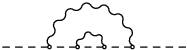
Here we can decompose $\langle\cdots\rangle$ into all possible contractions in case of the Gaussian average. Then, only the adjacent contraction making the tadpole diagram as shown in Fig. 2 (a) survives and other contractions as in Figs. 2 (b) and (c) vanish because of the delta-function in Eq. (5). Since the tadpole contribution is to be factorized as $\langle\rho_{a_{1}}\rho_{a_{2}}\cdots\rho_{a_{n}}\rangle=\langle\rho_{a_{1}}\rho_{a_{2}}\rangle\langle\rho_{a_{3}}\cdots\rho_{a_{n}}\rangle$ , we can rewrite Eq. (7) into a form of the integral equation;

	$\displaystyle\hskip-28.45274pt\bigl\langle U(b^{-},a^{-}\|\boldsymbol{x}_{\perp})_{\beta\alpha}\bigr\rangle=$	(8)
$\displaystyle=$	$\displaystyle\delta_{\beta\alpha}+(-\mathrm{i}g^{2})^{2}\int_{a^{-}}^{b^{-}}\!\mathrm{d}z_{1}^{-}\mathrm{d}^{2}\boldsymbol{z}_{1\perp}\int_{a^{-}}^{z_{1}^{-}}\!\mathrm{d}z_{2}^{-}\mathrm{d}^{2}\boldsymbol{z}_{2\perp}\,G_{0}(\boldsymbol{x}_{\perp}\!-\!\boldsymbol{z}_{1\perp})G_{0}(\boldsymbol{x}_{\perp}\!-\!\boldsymbol{z}_{2\perp})\times$
	$\displaystyle\times\bigl\langle\rho_{a_{1}}(z_{1}^{-},\boldsymbol{z}_{1\perp})\rho_{a_{2}}(z_{2}^{-},\boldsymbol{z}_{2\perp})\bigr\rangle\bigl(t^{a_{1}}t^{a_{2}}\bigr)_{\beta\gamma}\bigl\langle U(z_{2}^{-},a^{-}\|\boldsymbol{x}_{\perp})_{\gamma\alpha}\bigr\rangle$
$\displaystyle=$	$\displaystyle\delta_{\beta\alpha}-\frac{g^{4}}{2}C_{2}(r)\,\delta_{\beta\gamma}\int\mathrm{d}^{2}\boldsymbol{z}_{\perp}\,G_{0}^{2}(\boldsymbol{x}_{\perp}\!-\!\boldsymbol{z}_{\perp})\int^{b^{-}}_{a^{-}}\!\mathrm{d}z^{-}\mu^{2}(z^{-})\bigl\langle U(z^{-},a^{-}\|\boldsymbol{x}_{\perp})_{\gamma\alpha}\bigr\rangle\,,$

where we note that we used $\int^{z_{1}^{-}}_{a^{-}}\!\mathrm{d}z_{2}^{-}\,\delta(z_{1}^{-}\!-\!z_{2}^{-})=\frac{1}{2}$ and $(t^{a}t^{a})_{\beta\alpha}=C_{2}(r)\delta_{\beta\alpha}$ with the second-order Casimir invariant $C_{2}(r)$ in the $r$ representation.

We show the diagrammatic representation of this integral equation as

with the tadpole attached at $(z^{-},\boldsymbol{x}_{\perp})$ . We can easily find the solution, that is given by

\bigl\langle U(b^{-},a^{-}|\boldsymbol{x}_{\perp})_{\beta\alpha}\bigr\rangle=\bar{U}(b^{-},a^{-}|\boldsymbol{x}_{\perp})\,\delta_{\beta\alpha}=\exp\biggl[-Q_{\rm s}^{2}(b^{-},a^{-})\frac{2N_{\rm c}}{N_{\rm c}^{2}-1}\,C_{2}(r)\,L(x,x)\biggr]\,\delta_{\beta\alpha}\,,

(9)

where we defined

	$\displaystyle L(x,y)$	$\displaystyle=$	$\displaystyle g^{4}\int\mathrm{d}^{2}\boldsymbol{z}_{\perp}\,G_{0}(\boldsymbol{x}_{\perp}\!-\!\boldsymbol{z}_{\perp})\,G_{0}(\boldsymbol{y}_{\perp}\!-\!\boldsymbol{z}_{\perp})\,,$		(10)
	$\displaystyle Q_{\rm s}^{2}(b^{-},a^{-})$	$\displaystyle=$	$\displaystyle\frac{N_{\rm c}^{2}-1}{4N_{\rm c}}\int^{b^{-}}_{a^{-}}\!\mathrm{d}z^{-}\,\mu^{2}(z^{-})\,.$		(11)

Here we remark that we will simply write $Q_{\rm s}^{2}$ to denote $Q_{\rm s}^{2}(+\infty,-\infty)$ in later discussions. It should be mentioned that $L(x,x)$ does not depend on $x$ in fact because of translational invariance, and thus we can write it as $L(0,0)$ equivalently. As we will argue later, however, $L(x,y)$ generally suffers infrared singularity, and the expectation value (9) turns out to be negligible small. This observation intuitively corresponds to the fact that a single quark or gluon with non-trivial color charge would interact with color charge fluctuations inside the target at even far distance on the transverse plane. As a result of this long-ranged interaction (which should be cut off by either the target size or confining scale $\sim\varLambda_{\text{QCD}}^{-1}$ ), a quark or gluon is absorbed strongly in multiple scattering.

2.2 Two-point function; $\bigl\langle U(\boldsymbol{x}_{1\perp})_{\beta_{1}\alpha_{1}}U(\boldsymbol{x}_{2\perp})_{\beta_{2}\alpha_{2}}\bigr\rangle$

We shall next consider the two-point function of the Wilson lines. This is, in contrast to the one-point function, physically relevant if the projectile is a $q\bar{q}$ mesonic or $gg$ glueball-like state. Not only the tadpole diagrams consisting of Fig. 2 (a) but also the ladder diagrams structured with the sub-diagram Fig. 3 (a) contribute to the Gaussian average (see Fig. 4 for typical example). Any diagram containing the crossing sub-diagram as shown in Fig. 3 (b) vanishes in the same way as the nesting and overlapping ones displayed in Fig. 2. We can compute the Gaussian average of two Wilson lines diagrammatically by combining all the tadpole and ladder subparts up. The Dyson equation we need to solve is as follows;

The horizontal lines represent $\langle U(b^{-},a^{-}|\boldsymbol{x}_{\perp})\rangle$ involving all the tadpole contributions. We can literally convert the above graphical equation into the algebraic equation as

	$\displaystyle\hskip-28.45274pt\bigl\langle U(b^{-},a^{-}\|\boldsymbol{x}_{1\perp})_{\beta_{1}\alpha_{1}}U(b^{-},a^{-}\|\boldsymbol{x}_{2\perp})_{\beta_{2}\alpha_{2}}\bigr\rangle=$	(12)
$\displaystyle=$	$\displaystyle\bigl\langle U(b^{-},a^{-}\|\boldsymbol{x}_{1\perp})\bigr\rangle_{\beta_{1}\alpha_{1}}\bigl\langle U(b^{-},a^{-}\|\boldsymbol{x}_{2\perp})\bigr\rangle_{\beta_{2}\alpha_{2}}-$
	$\displaystyle-g^{4}\int^{b^{-}}_{a^{-}}\!\mathrm{d}z^{-}\,\bigl\langle U(b^{-},z^{-}\|\boldsymbol{x}_{1\perp})\bigr\rangle_{\beta_{1}\lambda_{1}}\bigl\langle U(b^{-},z^{-}\|\boldsymbol{x}_{2\perp})\bigr\rangle_{\beta_{2}\lambda_{2}}\,t^{a}_{\lambda_{1}\gamma_{1}}\,t^{a}_{\lambda_{2}\gamma_{2}}\,\mu^{2}(z^{-})\times$
	$\displaystyle\times\int\mathrm{d}\boldsymbol{z}_{\perp}^{2}G_{0}(\boldsymbol{x}_{1\perp}\!-\!\boldsymbol{z}_{\perp})G_{0}(\boldsymbol{x}_{2\perp}\!-\!\boldsymbol{z}_{\perp})\bigl\langle U(z^{-},a^{-}\|\boldsymbol{x}_{1\perp})_{\gamma_{1}\alpha_{1}}U(z^{-},a^{-}\|\boldsymbol{x}_{2\perp})_{\gamma_{2}\alpha_{2}}\bigr\rangle$
$\displaystyle=$	$\displaystyle\bar{U}(b^{-},a^{-}\|\boldsymbol{x}_{1\perp})\,\bar{U}(b^{-},a^{-}\|\boldsymbol{x}_{2\perp})\Biggl(\delta_{\beta_{1}\alpha_{1}}\delta_{\beta_{2}\alpha_{2}}-L(x_{1},x_{2})\times$
	$\displaystyle\qquad\times\int^{b^{-}}_{a^{-}}\!\mathrm{d}z^{-}\mu^{2}(z^{-})\,t^{a}_{\beta_{1}\gamma_{1}}\,t^{a}_{\beta_{2}\gamma_{2}}\frac{\langle U(z^{-},a^{-}\|\boldsymbol{x}_{1\perp})_{\gamma_{1}\alpha_{1}}U(z^{-},a^{-}\|\boldsymbol{x}_{2\perp})_{\gamma_{2}\alpha_{2}}\rangle}{\bar{U}(z^{-},a^{-}\|\boldsymbol{x}_{1\perp})\,\bar{U}(z^{-},a^{-}\|\boldsymbol{x}_{2\perp})}\Biggr)\,.$

We divide the both sides of this integral equation by $\bar{U}(b^{-},a^{-}|\boldsymbol{x}_{1\perp})\,\bar{U}(b^{-},a^{-}|\boldsymbol{x}_{2\perp})$ to reach

	$\displaystyle\hskip-28.45274ptF(\boldsymbol{x}_{1\perp},\boldsymbol{x}_{2\perp}\|b^{-},a^{-})_{\beta_{1}\beta_{2};\alpha_{1}\alpha_{2}}=$
	$\displaystyle\hskip-28.45274pt=\delta_{\beta_{1}\alpha_{1}}\delta_{\beta_{2}\alpha_{2}}-L(x_{1},x_{2})\int^{b^{-}}_{a^{-}}\!\mathrm{d}z^{-}\mu^{2}(z^{-})\,t^{a}_{\beta_{1}\gamma_{1}}\,t^{a}_{\beta_{2}\gamma_{2}}F(\boldsymbol{x}_{1\perp},\boldsymbol{x}_{2\perp}\|z^{-},a^{-})_{\gamma_{1}\gamma_{2};\alpha_{1}\alpha_{2}}\,,$		(13)

where we defined

F(\boldsymbol{x}_{1\perp},\boldsymbol{x}_{2\perp}|b^{-},a^{-})_{\beta_{1}\beta_{2};\alpha_{1}\alpha_{2}}=\frac{\langle U(b^{-},a^{-}|\boldsymbol{x}_{1\perp})_{\beta_{1}\alpha_{1}}\,U(b^{-},a^{-}|\boldsymbol{x}_{2\perp})_{\beta_{2}\alpha_{2}}\rangle}{\bar{U}(b^{-},a^{-}|\boldsymbol{x}_{1\perp})\,\bar{U}(b^{-},a^{-}|\boldsymbol{x}_{2\perp})}\,.

(14)

The integral equation (13) has an identical structure as Eq. (8), so that we can solve it in the same way to find

F(\boldsymbol{x}_{1\perp},\boldsymbol{x}_{2\perp}|b^{-},a^{-})_{\beta_{1}\beta_{2};\alpha_{1}\alpha_{2}}=\exp\biggl[-2Q_{\rm s}^{2}(b^{-},a^{-})\frac{2N_{\rm c}}{N_{\rm c}^{2}-1}t^{a}_{1}\,t^{a}_{2}\,L(x_{1},x_{2})\biggr]_{\beta_{1}\beta_{2};\alpha_{1}\alpha_{2}}\,.

(15)

In the limit of $a^{-}\to-\infty$ and $b^{-}\to+\infty$ , as a result, we can express the Wilson line average in the following form;

	$\displaystyle\hskip-28.45274pt\bigl\langle U(\boldsymbol{x}_{1\perp})_{\beta_{1}\alpha_{1}}U(\boldsymbol{x}_{2\perp})_{\beta_{2}\alpha_{2}}\bigr\rangle=$	(16)
$\displaystyle=$	$\displaystyle\bar{U}(\boldsymbol{x}_{1\perp})\bar{U}(\boldsymbol{x}_{2\perp})\exp\biggl[-2Q_{\rm s}^{2}\frac{2N_{\rm c}}{N_{\rm c}^{2}-1}t^{a}_{1}\,t^{a}_{2}\,L(x_{1},x_{2})\biggr]_{\beta_{1}\beta_{2};\alpha_{1}\alpha_{2}}$
$\displaystyle=$	$\displaystyle\exp\biggl[-Q_{\rm s}^{2}\frac{2N_{\rm c}}{N_{\rm c}^{2}-1}\Bigl(2t^{a}_{1}\,t^{a}_{2}\,L(x_{1},x_{2})+t^{a2}_{1}\,L(x_{1},x_{1})+t^{a2}_{2}\,L(x_{2},x_{2})\Bigr)\biggr]_{\beta_{1}\beta_{2};\alpha_{1}\alpha_{2}}$
$\displaystyle=$	$\displaystyle\exp\biggl[-Q_{\rm s}^{2}\frac{2N_{\rm c}}{N_{\rm c}^{2}-1}\Bigl((t^{a}_{1}+t^{a}_{2})^{2}L(0,0)-t^{a}_{1}\,t^{a}_{2}\varGamma(x_{1},x_{2})\Bigr)\biggr]_{\beta_{1}\beta_{2};\alpha_{1}\alpha_{2}}\,,$

where we made use of translational invariance to make a shift $L(x,x)\to L(0,0)$ and defined $\varGamma(x_{1},x_{2})=2(L(0,0)-L(x_{1},x_{2}))$ which is free from infrared singularity.

Here, let us introduce “Hamiltonian” by

\bigl\langle U(b^{-},a^{-}|\boldsymbol{x}_{1\perp})_{\beta_{1}\alpha_{1}}U(b^{-},a^{-}|\boldsymbol{x}_{2\perp})_{\beta_{2}\alpha_{2}}\bigr\rangle=\exp[-(H_{0}+V)]_{\beta_{1}\beta_{2};\alpha_{1}\alpha_{2}}

(17)

with the “free” part,

H_{0}=Q_{\rm s}^{2}\frac{2N_{\rm c}}{N_{\rm c}^{2}-1}(t^{a}_{1}+t^{a}_{2})^{2}L(0,0)\,,

(18)

and the “interaction” part,

V=-Q_{\rm s}^{2}\frac{2N_{\rm c}}{N_{\rm c}^{2}-1}\,t^{a}_{1}\,t^{a}_{2}\varGamma(x_{1},x_{2})\,.

(19)

One can readily prove that $[H_{0},V]=0$ meaning that $TH_{0}T^{-1}$ and $TVT^{-1}$ are to become diagonal simultaneously. Let us consider the decomposition of $H_{0}$ into irreducible representations in color space. We see that $H_{0}$ is proportional to the second-order Casimir operator $(t^{a}_{1}+t^{a}_{2})^{2}$ . In general the irreducible representation is labeled by a set of non-negative integers $m$ with rank $N_{\rm c}-1$ , i.e., Dynkin coefficients. The associated second-order Casimir invariant is expressed as

C_{2}(m)=\frac{1}{2N_{\rm c}}\Biggl[\sum_{n=1}^{N_{\rm c}-1}n(N_{\rm c}-n)(N_{\rm c}+m_{n})m_{n}+2\sum_{n>l}^{N_{\rm c}-1}l(N_{\rm c}-n)m_{n}\,m_{l}\Biggr]\,.

(20)

For example $C_{2}=4/3$ for the fundamental representation (triplet) of $\mathop{\rm SU}(N_{\rm c}=3)$ characterized by $m=[1,0]$ and $C_{2}=3$ for the adjoint representation (octet) characterized by $m=[1,1]$ . It is obvious from Eq. (20) that $C_{2}(m)$ is semi-positive and zero only when $m=0$ , that is, a singlet. If the color structure of the Wilson line correlator is projected onto non-singlet states, $H_{0}$ gives a large suppression factor, which can be seen from

$\displaystyle L(x,y)$	$\displaystyle=$	$\displaystyle g^{4}\int\mathrm{d}^{2}\boldsymbol{z}_{\perp}\,G_{0}(\boldsymbol{x}_{\perp}\!-\!\boldsymbol{z}_{\perp})\,G_{0}(\boldsymbol{y}_{\perp}\!-\!\boldsymbol{z}_{\perp})$	(21)
	$\displaystyle=$	$\displaystyle g^{4}\int\mathrm{d}^{2}\boldsymbol{z}_{\perp}\int\frac{\mathrm{d}^{2}\boldsymbol{k}_{\perp}}{(2\pi)^{2}}\;\mathrm{e}^{\mathrm{i}(\boldsymbol{x}_{\perp}-\boldsymbol{z}_{\perp})\cdot\boldsymbol{k}_{\perp}}\int\frac{\mathrm{d}^{2}\boldsymbol{q}_{\perp}}{(2\pi)^{2}}\;\mathrm{e}^{\mathrm{i}(\boldsymbol{y}_{\perp}-\boldsymbol{z}_{\perp})\cdot\boldsymbol{q}_{\perp}}\frac{1}{\boldsymbol{k}_{\perp}^{2}}\frac{1}{\boldsymbol{q}_{\perp}^{2}}$
	$\displaystyle=$	$\displaystyle g^{4}\int\frac{\mathrm{d}k\,\mathrm{d}\theta}{(2\pi)^{2}}\;\mathrm{e}^{\mathrm{i}\|\boldsymbol{y}_{\perp}-\boldsymbol{x}_{\perp}\|k\cos\theta}\frac{1}{k^{3}}$
	$\displaystyle=$	$\displaystyle g^{4}\int_{0}^{\infty}\frac{\mathrm{d}k}{2\pi}\,\frac{1}{k^{3}}\,J_{0}(k\|\boldsymbol{x}_{\perp}-\boldsymbol{y}_{\perp}\|)\,,$

where $J_{0}(x)$ is the first-kind Bessel function. When $k$ is small (strictly speaking, when $k|\boldsymbol{x}_{\perp}-\boldsymbol{y}_{\perp}|$ is small), $J_{0}(k|\boldsymbol{x}_{\perp}-\boldsymbol{y}_{\perp}|)\simeq 1-\frac{1}{4}(k|\boldsymbol{x}_{\perp}-\boldsymbol{y}_{\perp}|)^{2}$ , hence, the momentum integration in $L(x,y)$ infraredly diverges. We introduce an infrared cutoff $\varLambda_{\text{QCD}}$ to regularize the infrared singularity. Then, we have $L(x,y)\sim 1/\varLambda_{\text{QCD}}^{2}$ and $\varGamma(x,y)\sim|\boldsymbol{x}_{\perp}\!-\!\boldsymbol{y}_{\perp}|^{2}\ln(|\boldsymbol{x}_{\perp}\!-\!\boldsymbol{y}_{\perp}|\varLambda_{\text{QCD}})$ . Therefore, for small $\varLambda_{\text{QCD}}$ , $H_{0}$ which is proportional to $L(0,0)$ should be much larger than $V$ which is proportional to $\varGamma(x,y)$ . The non-singlet part in the color decomposition is thus accompanied by a large suppression factor, $\exp[-(2N_{\rm c}/(N_{\rm c}^{2}\!-\!1))C_{2}(m)Q_{\rm s}^{2}/(4\pi\varLambda_{\text{QCD}}^{2})]$ . This is a physically reasonable result; the Wilson lines form a color singlet, and such neutral objects are free from long-ranged color interactions (except for logarithmic singularity) which should be cut off by the confining scale $\varLambda_{\text{QCD}}^{-1}$ . Because $Q_{\rm s}$ (which is $\sim\mbox{GeV}$ order) is typically greater than $\varLambda_{\text{QCD}}\sim\mbox{fm}^{-1}$ by one order of magnitude at least, we do not have to concern non-singlet parts. From now on, accordingly, we consider only the singlet part of the color structure of the Wilson line product.

2.3 $n$ -point function; $\bigl\langle U(\boldsymbol{x}_{1\perp})_{\beta_{1}\alpha_{1}}U(\boldsymbol{x}_{2\perp})_{\beta_{2}\alpha_{2}}\cdots U(\boldsymbol{x}_{n\perp})_{\beta_{n}\alpha_{n}}\bigr\rangle$

Now that we have understood the computational procedure, it is easy to generalize the formulae to the $n$ -point case. The integral equation can be diagrammatically represented as

The R.H.S. consists of all the possible permutations of one ladder bridging over two out of $n$ Wilson lines. The horizontal lines are $\langle U(b^{-},a^{-}|\boldsymbol{x}_{\perp})\rangle$ with all the tadpole insertions. The corresponding equation is

	$\displaystyle\hskip-28.45274pt\bigl\langle U(b^{-},a^{-}\|\boldsymbol{x}_{1\perp})_{\beta_{1}\alpha_{1}}U(b^{-},a^{-}\|\boldsymbol{x}_{2\perp})_{\beta_{2}\alpha_{2}}\cdots U(b^{-},a^{-}\|\boldsymbol{x}_{n\perp})_{\beta_{n}\alpha_{n}}\bigr\rangle$	(22)
$\displaystyle=$	$\displaystyle\prod_{i=1}^{n}\bigl\langle U(b^{-},a^{-}\|\boldsymbol{x}_{i\perp})\bigr\rangle_{\beta_{i}\alpha_{i}}-g^{4}\sum_{i>j}\int^{b^{-}}_{a^{-}}\!\mathrm{d}z^{-}\mu^{2}(z^{-})\int\mathrm{d}\boldsymbol{z}_{\perp}^{2}\,G_{0}(\boldsymbol{x}_{i\perp}\!-\!\boldsymbol{z}_{\perp})\,G_{0}(\boldsymbol{x}_{j\perp}\!-\!\boldsymbol{z}_{\perp})\times$
	$\displaystyle\times\prod_{k=1}^{n}\bigl\langle U(b^{-},z^{-}\|\boldsymbol{x}_{i\perp})\bigr\rangle_{\beta_{k}\lambda_{k}}\,\delta_{\lambda_{1}\gamma_{1}}\cdots\delta_{\lambda_{j-1}\gamma_{j-1}}\,t^{a}_{\lambda_{j}\gamma_{j}}\,\delta_{\lambda_{j+1}\gamma_{j+1}}\cdots$
	$\displaystyle\cdots\delta_{\lambda_{i-1}\gamma_{i-1}}\,t^{a}_{\lambda_{i}\gamma_{i}}\delta_{\lambda_{i+1}\gamma_{i+1}}\cdots\delta_{\lambda_{n}\gamma_{n}}\times$
	$\displaystyle\times\bigl\langle U(z^{-},a^{-}\|\boldsymbol{x}_{1\perp})_{\gamma_{1}\alpha_{1}}U(z^{-},a^{-}\|\boldsymbol{x}_{2\perp})_{\gamma_{2}\alpha_{2}}\cdots U(a^{-},z^{-}\|\boldsymbol{x}_{n\perp})_{\gamma_{n}\alpha_{n}}\bigr\rangle\,.$

The above integral equation takes a similar form to the case of two-point function in Eq. (12), so that we can find the solution in the same way as

\bigl\langle U(\boldsymbol{x}_{1\perp})_{\beta_{1}\alpha_{1}}U(\boldsymbol{x}_{2\perp})_{\beta_{2}\alpha_{2}}\cdots U(\boldsymbol{x}_{n\perp})_{\beta_{n}\alpha_{n}}\bigr\rangle=\exp[-(H_{0}+V)]_{\beta_{1}\cdots\beta_{n};\alpha_{1}\cdots\alpha_{n}}

(23)

with

	$\displaystyle H_{0}$	$\displaystyle=$	$\displaystyle Q_{\rm s}^{2}\frac{2N_{\rm c}}{N_{\rm c}^{2}-1}\biggl(\sum_{k=1}^{n}t_{k}^{a}\biggr)^{2}L(0,0)\,,$		(24)
	$\displaystyle V$	$\displaystyle=$	$\displaystyle-Q_{\rm s}^{2}\frac{2N_{\rm c}}{N_{\rm c}^{2}-1}\sum_{i>j}\,t^{a}_{i}\,t^{a}_{j}\;\varGamma(\boldsymbol{x}_{i\perp},\boldsymbol{x}_{j\perp})\,.$		(25)

These expressions are plain generalization of Eqs. (18) and (19). Again, $H_{0}$ is proportional to the second-order Casimir operator, and after decomposing the color structure into irreducible representations, we can drop non-singlet parts. What we should do to simplify the result further is find the singlets out of the direct product of $\mathop{\rm SU}(N_{\rm c})$ matrices which make $H_{0}$ vanishing. For example, in case of the four-point function of Wilson lines in the adjoint representation with $N_{\rm c}=3$ (i.e. four gluon propagation through a dense target), there are eight independent singlets out of $8\otimes 8\otimes 8\otimes 8$ . Thus, the Wilson line correlator can be expressed to be an $8\times 8$ matrix of $\mathrm{e}^{-V}$ in the basis of eight singlets. We will face with concrete calculations later. In most cases of our interest in physics problems, all we need to know is expressed in terms of its eigenvalues and eigenstates.

3 Examples

We will elaborate several concrete examples relevant to physical processes. We will identify the singlet basis to compute the eigenvalue of the color matrix.

3.1 $\langle U(\boldsymbol{x}_{1\perp})_{\beta_{1}\alpha_{1}}U^{\ast}(\boldsymbol{x}_{2\perp})_{\beta_{2}\alpha_{2}}\rangle$ in the fundamental representation

In our formulae (18) and (19) we set $t_{1}^{a}=T_{\text{F}}^{a}$ and $t^{a}_{2}=-T_{\text{F}}^{a\ast}$ where $T_{\text{F}}^{a}$ ’s are the $\mathop{\rm SU}(N_{\rm c})$ generator in the fundamental representation. This expectation value appears in one color dipole or $q\bar{q}$ scattering off a dense target. In this case the number of singlet is only one; $N_{\rm c}\otimes N_{\rm c}^{\ast}=1\oplus N_{\rm c}^{2}-1$ . If we denote the singlet state as $|s\rangle$ then we have $\langle\alpha_{1}\alpha_{2}|s\rangle=\delta_{\alpha_{1}\alpha_{2}}/\sqrt{N_{\rm c}}$ with a proper normalization. The projected element of the necessary part is

\langle s|V|s\rangle=Q_{\rm s}^{2}\frac{2N_{\rm c}}{N_{\rm c}^{2}-1}\,{T_{\text{F}}}^{a}_{\beta_{1}\alpha_{1}}\,{T_{\text{F}}}^{\ast a}_{\beta_{2}\alpha_{2}}\,\varGamma(x_{1},x_{2})\,\frac{\delta_{\alpha_{1}\alpha_{2}}\delta_{\beta_{1}\beta_{2}}}{N_{\rm c}}=Q_{\rm s}^{2}\,\varGamma(x_{1},x_{2})\,.

(26)

Consequently, the singlet part of the two-point function of Wilson lines in the fundamental representation is

\bigl\langle U(\boldsymbol{x}_{1\perp})_{\beta_{1}\alpha_{1}}U^{\ast}(\boldsymbol{x}_{2\perp})_{\beta_{2}\alpha_{2}}\bigr\rangle=\exp\bigl[-Q_{\rm s}^{2}\,\varGamma(x_{1},x_{2})\bigr]\,\delta_{\beta_{1}\beta_{2}}\,\delta_{\alpha_{1}\alpha_{2}}/N_{\rm c}\,,

(27)

which means that only the closed color dipole survives under the average over random color distribution inside a dense gluon medium.

3.2 $\langle U(\boldsymbol{x}_{1\perp})_{\beta_{1}\alpha_{1}}U(\boldsymbol{x}_{2\perp})_{\beta_{2}\alpha_{2}}\rangle$ in the general representation

It is possible to extend the previous argument formally. We can reach a more general expression in arbitrary representation. The direct product of two irreducible representations, $r_{1}$ and $r_{2}$ , makes one singlet when $r_{2}$ is the star representation to $r_{1}$ , that is, $r_{1}=r_{2}^{*}=r$ , leading to the generators, $t_{2}^{a}=-t_{1}^{a*}$ . In this general case we have $\langle\alpha_{1}\alpha_{2}|s\rangle=\delta_{\alpha_{1}\alpha_{2}}/\sqrt{d_{r}}$ , where $d_{r}$ is the dimension of $r$ representation, which is given by the Dynkin coefficients $m$ charactering the irreducible representation $r$ as

d_{r}(m)=\prod_{i<j}^{N_{\rm c}}\Biggl(1+\sum_{n=i}^{j-1}\frac{m_{n}}{j-i}\Biggr)\,.

(28)

We can express $t^{a}_{1}t_{2}^{a}$ using the Casimir invariant;

t^{a}_{1}\,t_{2}^{a}=\frac{1}{2}\bigl[(t^{a}_{1}+t^{a}_{2})^{2}-(t_{1}^{a})^{2}-(t_{2}^{a})^{2}\bigr]=-\frac{1}{2}\bigl[C_{2}(r_{1})+C_{2}(r_{2})\bigr]=-C_{2}(r)\,,

(29)

leading to

\langle s|V|s\rangle=Q_{\rm s}^{2}\frac{2N_{\rm c}}{N_{\rm c}^{2}-1}\,C_{2}(r)\,\varGamma(x_{1},x_{2})\,.

(30)

After all, the generalization of Eq. (27) takes an expression of

\bigl\langle U(\boldsymbol{x}_{1\perp})_{\beta_{1}\alpha_{1}}U(\boldsymbol{x}_{2\perp})_{\beta_{2}\alpha_{2}}\bigr\rangle=\exp\biggl[-Q_{\rm s}^{2}\,\frac{2N_{\rm c}}{N_{\rm c}^{2}-1}\,C_{2}(r)\,\varGamma(x_{1},x_{2})\biggr]\,\delta_{\beta_{1}\alpha_{1}}\,\delta_{\beta_{2}\alpha_{2}}/d_{r}\,.

(31)

3.3 $\langle U(\boldsymbol{x}_{1\perp})_{\alpha_{1}\beta_{1}}U(\boldsymbol{x}_{2\perp})_{\alpha_{2}\beta_{2}}\cdots U(\boldsymbol{x}_{N_{\rm c}\perp})_{\alpha_{N_{\rm c}}\beta_{N_{\rm c}}}\rangle$ in the fundamental representation

This expectation value is relevant to the scattering amplitude between a baryon consisting of $N_{\rm c}$ valence quarks and dense gluon matter inside a heavy hadron. One can find an example of the baryon expectation value in the context of the Odderon physics [14, 15], though the Gaussian average can only describe the Pomeron part.

The singlet state with one baryon is $\langle\alpha_{1}\cdots\alpha_{n}|s\rangle=\epsilon_{\alpha_{1}\alpha_{2}\cdots\alpha_{N_{\rm c}}}/\sqrt{N_{\rm c}!}$ where $\epsilon_{\alpha_{1}\alpha_{2}\cdots\alpha_{N_{\rm c}}}$ is the antisymmetric tensor with the definition $\epsilon_{12\cdots N_{\rm c}}=1$ . The matrix element $\langle s|{T_{\text{F}}}^{a}_{i}{T_{\text{F}}}^{a}_{j}|s\rangle$ does not depend on the indices, $i$ and $j$ , that is,

\langle s|{T_{\text{F}}}^{a}_{i}\,{T_{\text{F}}}^{a}_{j}|s\rangle=-\frac{{T_{\text{F}}}^{a}_{\beta\alpha}{T_{\text{F}}}^{a}_{\alpha\beta}}{N_{\rm c}!}\,(N_{\rm c}-2)!=-\frac{N_{\rm c}+1}{2N_{\rm c}}\,,

(32)

that yields

\langle s|V|s\rangle=Q_{\rm s}^{2}\,\frac{1}{N_{\rm c}-1}\sum_{i>j}\,\varGamma(\boldsymbol{x}_{i\perp},\boldsymbol{x}_{j\perp})\,.

(33)

The baryon expectation value is thus,

	$\displaystyle\displaystyle\bigl\langle U(\boldsymbol{x}_{1\perp})_{\beta_{1}\alpha_{1}}U(\boldsymbol{x}_{2\perp})_{\beta_{2}\alpha_{2}}\cdots U(\boldsymbol{x}_{N_{\rm c}\perp})_{\beta_{N_{\rm c}}\alpha_{N_{\rm c}}}\bigr\rangle=\qquad\qquad$
	$\displaystyle\displaystyle\qquad\qquad=\exp\biggl[-Q_{\rm s}^{2}\,\frac{1}{N_{\rm c}-1}\sum_{i>j}\,\varGamma(\boldsymbol{x}_{i\perp},\boldsymbol{x}_{j\perp})\biggr]\frac{\epsilon_{\alpha_{1}\alpha_{2}\cdots\alpha_{N_{\rm c}}}\epsilon_{\beta_{1}\beta_{2}\cdots\beta_{N_{\rm c}}}}{N_{\rm c}!}\,.$		(34)

When $N_{\rm c}$ gets large, the exponential factor is decreasing in contrast to the meson scattering in Eq. (27) that stays unsuppressed for large $N_{\rm c}$ . This is a manifestation of the fact that baryons would not live as they are in the large- $N_{\rm c}$ limit but mesons would.

3.4 $\langle\tilde{U}(\boldsymbol{x}_{1\perp})_{\beta_{1}\alpha_{1}}\tilde{U}(\boldsymbol{x}_{2\perp})_{\beta_{2}\alpha_{2}}\tilde{U}(\boldsymbol{x}_{3\perp})_{\beta_{3}\alpha_{3}}\rangle$ in the adjoint representation

So far, the number of singlet is only one, and the next step we are heading for is to treat the case with multiple singlets. The simplest and still non-trivial is the three gluon propagation, in which $(N_{\rm c}^{2}-1)\otimes(N_{\rm c}^{2}-1)\otimes(N_{\rm c}^{2}-1)$ includes two singlets composed of $f_{abc}=-2\mathrm{i}\mathop{\rm tr}([T_{\text{A}}^{a},T_{\text{A}}^{b}]T_{\text{A}}^{c})$ and $d_{abc}=2\mathop{\rm tr}(\{T_{\text{A}}^{a},T_{\text{A}}^{b}\}T_{\text{A}}^{c})$ , where $T_{\text{A}}^{a}$ ’s represent the $\mathop{\rm SU}(N_{\rm c})$ generator in the adjoint representation, as

	$\displaystyle\langle\alpha_{1}\alpha_{2}\alpha_{3}\|s_{1}\rangle$	$\displaystyle=$	$\displaystyle f_{\alpha_{1}\alpha_{2}\alpha_{3}}\frac{1}{\sqrt{(N_{\rm c}^{2}-1)N_{\rm c}}}\,,$
	$\displaystyle\langle\alpha_{1}\alpha_{2}\alpha_{3}\|s_{2}\rangle$	$\displaystyle=$	$\displaystyle d_{\alpha_{1}\alpha_{2}\alpha_{3}}\,\sqrt{\frac{N_{\rm c}}{(N_{\rm c}^{2}-4)(N_{\rm c}^{2}-1)}}$		(35)

with a proper normalization. Using the Jacobi identities, $f_{abe}f_{cde}+f_{ade}f_{bce}+f_{ace}f_{dbe}=0$ and $f_{abe}d_{cde}+f_{ade}d_{bce}+f_{ace}d_{dbe}=0$ we can calculate each matrix element in singlet space as

$\displaystyle\langle s_{1}\|{T_{\text{A}}}^{a}_{i}\,{T_{\text{A}}}^{a}_{j}\|s_{1}\rangle$	$\displaystyle=$	$\displaystyle-f_{\alpha_{1}\,a\,\beta_{1}}f_{\alpha_{2}\,a\,\beta_{2}}f_{\alpha_{1}\alpha_{2}\beta_{3}}f_{\beta_{1}\beta_{2}\beta_{3}}\,\frac{1}{N_{\rm c}(N_{\rm c}^{2}-1)}=-\frac{N_{\rm c}}{2}\,,$
$\displaystyle\langle s_{1}\|{T_{\text{A}}}^{a}_{i}\,{T_{\text{A}}}^{a}_{j}\|s_{2}\rangle$	$\displaystyle=$	$\displaystyle-f_{\alpha_{1}\,a\,\beta_{1}}f_{\alpha_{2}\,a\,\beta_{2}}f_{\alpha_{1}\alpha_{2}\beta_{3}}d_{\beta_{1}\beta_{2}\beta_{3}}\,\frac{1}{(N_{\rm c}^{2}-1)\sqrt{N_{\rm c}^{2}-4}}=0\,,$
$\displaystyle\langle s_{2}\|{T_{\text{A}}}^{a}_{i}\,{T_{\text{A}}}^{a}_{j}\|s_{2}\rangle$	$\displaystyle=$	$\displaystyle-f_{\alpha_{1}\,a\,\beta_{1}}f_{\alpha_{2}\,a\,\beta_{2}}d_{\alpha_{1}\alpha_{2}\beta_{3}}d_{\beta_{1}\beta_{2}\beta_{3}}\,\frac{N_{\rm c}}{(N_{\rm c}^{2}-4)(N_{\rm c}^{2}-1)}=-\frac{N_{\rm c}}{2}\,,$	(36)

which are independent of the indices $i$ and $j$ , and thus the matrix structure is simply proportional to unity. The projected $V$ is then,

V=Q_{\rm s}^{2}\,\frac{N_{\rm c}^{2}}{N_{\rm c}^{2}-1}\sum_{i>j}\,\varGamma(\boldsymbol{x}_{i\perp},\boldsymbol{x}_{j\perp})\begin{pmatrix}1&0\\ 0&1\end{pmatrix}\,.

(37)

At last, we get the result,

	$\displaystyle\bigl\langle\tilde{U}(\boldsymbol{x}_{1\perp})_{\beta_{1}\alpha_{1}}\tilde{U}(\boldsymbol{x}_{2\perp})_{\beta_{2}\alpha_{2}}\tilde{U}(\boldsymbol{x}_{3\perp})_{\beta_{3}\alpha_{3}}\bigr\rangle$	$\displaystyle=$	$\displaystyle\frac{1}{N_{\rm c}(N_{\rm c}^{2}-1)}\,\exp\biggl[-Q_{\rm s}^{2}\,\frac{N_{\rm c}^{2}}{N_{\rm c}^{2}-1}\sum_{i>j}\,\varGamma(\boldsymbol{x}_{i\perp},\boldsymbol{x}_{j\perp})\biggr]\times$		(38)
			$\displaystyle\times\biggl(f_{\alpha_{1}\alpha_{2}\alpha_{3}}f_{\beta_{1}\beta_{2}\beta_{3}}+\frac{N_{\rm c}^{2}}{N_{\rm c}^{2}\!-\!4}d_{\alpha_{1}\alpha_{2}\alpha_{3}}d_{\beta_{1}\beta_{2}\beta_{3}}\biggr)\,.$		(38)

Roughly speaking, three gluons can make two kinds of color singlet glueballs and they do not mix together due to different symmetry. The first and second terms in the curly parenthesis are contributions from those glueball states respectively.

3.5 $\langle U(\boldsymbol{x}_{1\perp})_{\beta_{1}\alpha_{1}}U^{\ast}(\boldsymbol{x}_{2\perp})_{\beta_{2}\alpha_{2}}U(\boldsymbol{x}_{3\perp})_{\beta_{3}\alpha_{3}}U^{\ast}(\boldsymbol{x}_{4\perp})_{\beta_{4}\alpha_{4}}\rangle$ in the fundamental representation

The next non-trivial example is the four-point Wilson lines in the fundamental representation. This problem reduces to the irreducible decomposition of $N_{\rm c}\otimes N_{\rm c}^{\ast}\otimes N_{\rm c}\otimes N_{\rm c}^{\ast}$ , which contains two normalized singlets;

	$\displaystyle\langle\alpha_{1}\alpha_{2}\alpha_{3}\alpha_{4}\|s_{1}\rangle$	$\displaystyle=$	$\displaystyle\frac{1}{N_{\rm c}}\,\delta_{\alpha_{1}\alpha_{2}}\delta_{\alpha_{3}\alpha_{4}}\,,$
	$\displaystyle\langle\alpha_{1}\alpha_{2}\alpha_{3}\alpha_{4}\|s_{2}\rangle$	$\displaystyle=$	$\displaystyle\frac{1}{\sqrt{N_{\rm c}^{2}-1}}\biggl(\delta_{\alpha_{1}\alpha_{4}}\delta_{\alpha_{2}\alpha_{3}}-\frac{1}{N_{\rm c}}\,\delta_{\alpha_{1}\alpha_{2}}\delta_{\alpha_{3}\alpha_{4}}\biggr)\,,$		(39)

leading to the projected matrix elements of

	$\displaystyle V$	$\displaystyle=$	$\displaystyle-Q_{\rm s}^{2}\,\frac{2N_{\rm c}}{N_{\rm c}^{2}-1}\Bigl(-{T_{\text{F}}}^{a}_{1}\,{T_{\text{F}}}^{a\ast}_{2}\,\varGamma(\boldsymbol{x}_{1\perp},\boldsymbol{x}_{2\perp})+{T_{\text{F}}}^{a}_{1}\,{T_{\text{F}}}^{a}_{3}\,\varGamma(\boldsymbol{x}_{1\perp},\boldsymbol{x}_{3\perp})-{T_{\text{F}}}^{a}_{1}\,{T_{\text{F}}}^{a\ast}_{4}\,\varGamma(\boldsymbol{x}_{1\perp},\boldsymbol{x}_{4\perp})-$		(40)
			$\displaystyle-{T_{\text{F}}}^{a\ast}_{2}\,{T_{\text{F}}}^{a}_{3}\,\varGamma(\boldsymbol{x}_{2\perp},\boldsymbol{x}_{3\perp})+{T_{\text{F}}}^{a\ast}_{2}\,{T_{\text{F}}}^{a\ast}_{4}\,\varGamma(\boldsymbol{x}_{2\perp},\boldsymbol{x}_{4\perp})-{T_{\text{F}}}^{a}_{3}\,{T_{\text{F}}}^{a\ast}_{4}\,\varGamma(\boldsymbol{x}_{3\perp},\boldsymbol{x}_{4\perp})\Bigr)\,,$		(40)

given by

\begin{pmatrix}V_{11}&V_{12}\\ V_{21}&V_{22}\end{pmatrix}=-Q_{\rm s}^{2}\,\frac{2N_{\rm c}}{N_{\rm c}^{2}-1}\begin{pmatrix}\displaystyle-\frac{N_{\rm c}^{2}-1}{N_{\rm c}}\gamma&\displaystyle\frac{\sqrt{N_{\rm c}^{2}-1}}{N_{\rm c}}\bigl(\beta-\alpha\bigr)\\ \displaystyle\frac{\sqrt{N_{\rm c}^{2}-1}}{N_{\rm c}}\bigl(\beta-\alpha\bigr)&\displaystyle\qquad\frac{1}{N_{\rm c}}\Bigl(\gamma-2\beta+(2-N_{\rm c}^{2})\alpha\Bigr)\end{pmatrix}\,,

(41)

where we defined with slight modification from Ref. [9]

$\displaystyle 2\alpha$	$\displaystyle=$	$\displaystyle\varGamma(\boldsymbol{x}_{1\perp},\boldsymbol{x}_{4\perp})+\varGamma(\boldsymbol{x}_{2\perp},\boldsymbol{x}_{3\perp})\,,$
$\displaystyle 2\beta$	$\displaystyle=$	$\displaystyle\varGamma(\boldsymbol{x}_{1\perp},\boldsymbol{x}_{3\perp})+\varGamma(\boldsymbol{x}_{2\perp},\boldsymbol{x}_{4\perp})\,,$	(42)
$\displaystyle 2\gamma$	$\displaystyle=$	$\displaystyle\varGamma(\boldsymbol{x}_{1\perp},\boldsymbol{x}_{2\perp})+\varGamma(\boldsymbol{x}_{3\perp},\boldsymbol{x}_{4\perp})\,,$

which are free from infrared singularity. In order to calculate the matrix element of $\exp(-V)$ , we need to diagonalize $V$ whose eigenvalues are given as the solution of the characteristic equation $\det[\lambda-V]=0$ , which gives us two eigenvalues,

\lambda_{\pm}=\frac{1}{2}\bigl(\mathop{\rm tr}V\pm\varphi\bigr)

(43)

with

\varphi=\sqrt{(\mathop{\rm tr}V)^{2}-4\det V}=Q_{\rm s}^{2}\frac{2N_{\rm c}^{2}}{N_{\rm c}^{2}-1}\sqrt{(\alpha-\gamma)^{2}+\frac{4}{N_{\rm c}^{2}}(\beta-\alpha)(\beta-\gamma)}

(44)

in our notation. The eigenstates are

u_{+}=\begin{pmatrix}\cos\theta\\ \sin\theta\end{pmatrix}\,,\qquad u_{-}=\begin{pmatrix}-\sin\theta\\ \cos\theta\end{pmatrix}\,,

(45)

with

\tan\theta=\frac{2V_{12}}{V_{11}-V_{22}+\varphi}\,.

(46)

Using the unitary matrix $T=(u_{+}\;u_{-})$ we can diagonalize $\exp(-V)$ to have

$\displaystyle\mathrm{e}^{-V}$	$\displaystyle=$	$\displaystyle T\begin{pmatrix}\mathrm{e}^{-\lambda_{+}}&0\\ 0&\mathrm{e}^{-\lambda_{-}}\end{pmatrix}T^{-1}$	(47)
	$\displaystyle=$	$\displaystyle\mathrm{e}^{-\frac{1}{2}\mathop{\rm tr}V}T\begin{pmatrix}\mathrm{e}^{-\frac{1}{2}\varphi}&0\\ 0&\mathrm{e}^{\frac{1}{2}\varphi}\end{pmatrix}T^{-1}$
	$\displaystyle=$	$\displaystyle\mathrm{e}^{-\frac{1}{2}\mathop{\rm tr}V}\begin{pmatrix}\cosh{\scriptstyle\frac{1}{2}}\varphi-(\cos^{2}\theta-\sin^{2}\theta)\sinh{\scriptstyle\frac{1}{2}}\varphi&-2\cos\theta\sin\theta\sinh{\scriptstyle\frac{1}{2}}\varphi\\ -2\cos\theta\sin\theta\sinh{\scriptstyle\frac{1}{2}}\varphi&\cosh{\scriptstyle\frac{1}{2}}\varphi+(\cos^{2}\theta-\sin^{2}\theta)\sinh{\scriptstyle\frac{1}{2}}\varphi\end{pmatrix}$
	$\displaystyle=$	$\displaystyle\mathrm{e}^{-\frac{1}{2}\mathop{\rm tr}V}\Biggl[\cosh{\scriptstyle\frac{1}{2}}\varphi-\frac{\sinh{\scriptstyle\frac{1}{2}}\varphi}{\varphi}\begin{pmatrix}V_{11}-V_{22}&2V_{12}\\ 2V_{12}&-V_{11}+V_{22}\end{pmatrix}\Biggr]\,.$

We can find one direct application of this example in the quark production from the CGC background in the p-A collision [9], in which the necessary quantity is

			$\displaystyle\hskip-28.45274pt\bigl\langle\mathop{\rm tr}\bigl\{U(\boldsymbol{x}_{1\perp})\,T_{\text{F}}^{a}\,U^{\dagger}(\boldsymbol{x}_{2\perp})\,U(\boldsymbol{x}_{3\perp})\,T_{\text{F}}^{a}\,U^{\dagger}(\boldsymbol{x}_{4\perp})\bigr\}\bigr\rangle=$		(48)
		$\displaystyle=$	$\displaystyle{T_{\text{F}}}^{a}_{\beta_{1}\beta_{2}}{T_{\text{F}}}^{a}_{\beta_{3}\beta_{4}}\delta_{\alpha_{2}\alpha_{3}}\delta_{\alpha_{4}\alpha_{1}}\bigl\langle U(\boldsymbol{x}_{1\perp})_{\alpha_{1}\beta_{1}}U^{\ast}(\boldsymbol{x}_{2\perp})_{\alpha_{2}\beta_{2}}U(\boldsymbol{x}_{3\perp})_{\alpha_{3}\beta_{3}}U^{\ast}(\boldsymbol{x}_{4\perp})_{\alpha_{4}\beta_{4}}\bigr\rangle\,.$		(48)

The color structure in ${T_{\text{F}}}^{a}_{\beta_{1}\beta_{2}}{T_{\text{F}}}^{a}_{\beta_{3}\beta_{4}}\delta_{\alpha_{2}\alpha_{3}}\delta_{\alpha_{4}\alpha_{1}}$ is to be expressed in terms of the singlet basis of Eq. (39) as follows;

	$\displaystyle{T_{\text{F}}}^{a}_{\beta_{1}\beta_{2}}{T_{\text{F}}}^{a}_{\beta_{3}\beta_{4}}\,\delta_{\alpha_{2}\alpha_{3}}\,\delta_{\alpha_{4}\alpha_{1}}=$
	$\displaystyle\qquad=\frac{\sqrt{N_{\rm c}^{2}-1}}{2}\langle\beta_{1}\beta_{2}\beta_{3}\beta_{4}\|s_{2}\rangle\Bigl(\sqrt{N_{\rm c}^{2}-1}\langle s_{2}\|\alpha_{1}\alpha_{2}\alpha_{3}\alpha_{4}\rangle+\langle s_{1}\|\alpha_{1}\alpha_{2}\alpha_{3}\alpha_{4}\rangle\Bigr)\,.$		(49)

Thus we immediately conclude

	$\displaystyle\hskip-28.45274pt\bigl\langle\mathop{\rm tr}\bigl\{U(\boldsymbol{x}_{1\perp})\,T_{\text{F}}^{a}\,U^{\dagger}(\boldsymbol{x}_{2\perp})\,U(\boldsymbol{x}_{3\perp})\,T_{\text{F}}^{a}\,U^{\dagger}(\boldsymbol{x}_{4\perp})\bigr\}\bigr\rangle=$	(50)
$\displaystyle=$	$\displaystyle\frac{N_{\rm c}^{2}-1}{2}\biggl(\langle s_{2}\|\mathrm{e}^{-V}\|s_{2}\rangle+\frac{1}{\sqrt{N_{\rm c}^{2}-1}}\langle s_{1}\|\mathrm{e}^{-V}\|s_{2}\rangle\biggr)$
$\displaystyle=$	$\displaystyle\frac{N_{\rm c}^{2}-1}{2}\,\mathrm{e}^{-\frac{1}{2}\mathop{\rm tr}V}\biggl[\cosh{\scriptstyle\frac{1}{2}}\varphi-\frac{\sinh{\scriptstyle\frac{1}{2}}\varphi}{\varphi}\Bigl(V_{22}-V_{11}+\frac{2}{\sqrt{N_{\rm c}^{2}-1}}V_{12}\Bigr)\biggr]$
$\displaystyle=$	$\displaystyle\frac{N_{\rm c}^{2}\!-\!1}{2}\mathrm{e}^{-Q_{\rm s}^{2}\frac{N_{\rm c}^{2}}{N_{\rm c}^{2}-1}\bigl[-(\alpha+\gamma)+\frac{2}{N_{\rm c}^{2}}(\alpha+\gamma-\beta)\bigr]}\!\biggl[\cosh\!{\scriptstyle\frac{1}{2}}\varphi+\frac{Q_{\rm s}^{2}}{\varphi}\,\frac{2N_{\rm c}^{2}}{N_{\rm c}^{2}\!-\!1}(\gamma\!-\!\alpha)\sinh\!{\scriptstyle\frac{1}{2}}\varphi\biggr].$

In order to compare this result to Eq. (86) in Ref. [9], we note that $Q_{\rm s}^{2}=(N_{\rm c}^{2}-1)/(4N_{\rm c})\mu_{A}^{2}$ and $\varphi={\scriptstyle\frac{1}{2}}N_{\rm c}\mu_{A}^{2}|\alpha-\gamma|\sqrt{\Delta}$ if written with the notation of Ref. [9]. Then, our result (50) turns out to agree exactly with Ref. [9].

3.6 $\langle\tilde{U}(\boldsymbol{x}_{1\perp})_{\beta_{1}\alpha_{1}}\tilde{U}(\boldsymbol{x}_{2\perp})_{\beta_{2}\alpha_{2}}\tilde{U}(\boldsymbol{x}_{3\perp})_{\beta_{3}\alpha_{3}}\tilde{U}(\boldsymbol{x}_{4\perp})_{\beta_{4}\alpha_{4}}\rangle$ in the adjoint representation

This quantity is, literally speaking, the four-gluon scattering amplitude. Also, in the calculation of two-gluon production from the CGC background [11], we have to evaluate $\mathop{\rm tr}\{\tilde{U}\,T_{\text{A}}^{a}\,\tilde{U}^{\dagger}\tilde{U}\,T_{\text{A}}^{a}\,\tilde{U}^{\dagger}\bigr\}$ in the adjoint representation. There are eight singlets [16] given by combinations of the following bases;

	$\displaystyle\delta_{\alpha_{1}\alpha_{2}}\delta_{\alpha_{3}\alpha_{4}}\,,\qquad\delta_{\alpha_{1}\alpha_{3}}\delta_{\alpha_{2}\alpha_{4}}\,,\qquad\delta_{\alpha_{1}\alpha_{4}}\delta_{\alpha_{2}\alpha_{3}}\,,$
	$\displaystyle d^{\alpha_{1}\alpha_{2}\gamma}d^{\alpha_{3}\alpha_{4}\gamma}\,,\qquad d^{\alpha_{1}\alpha_{3}\gamma}d^{\alpha_{2}\alpha_{4}\gamma}\,,$		(51)
	$\displaystyle d^{\alpha_{1}\alpha_{2}\gamma}f^{\alpha_{3}\alpha_{4}\gamma}\,,\qquad d^{\alpha_{1}\alpha_{3}\gamma}f^{\alpha_{2}\alpha_{4}\gamma}\,,\qquad d^{\alpha_{1}\alpha_{4}\gamma}f^{\alpha_{2}\alpha_{3}\gamma}\,.$

These states are not orthogonal, and it is very hard to obtain the eigenvalues and eigenstates of an $8\times 8$ matrix $V$ to compute $\mathrm{e}^{-V}$ . In the next section, we will develop an approximation to simplify the calculation.

4 Large- $N_{\rm c}$ limit

It is possible to construct any higher-dimensional representation from the direct product of the fundamental (and anti-fundamental) representation. A well-known example is the adjoint representation whose matrix representation can be given in terms of the fundamental Wilson lines as $2\mathrm{tr}[U(\boldsymbol{x}_{\perp})\,t^{\beta}U^{\dagger}(\boldsymbol{x}_{\perp})\,t^{\alpha}]$ where $\alpha$ and $\beta$ run from one to $N_{\rm c}^{2}-1$ . Here we shall consider the arbitrary product of $U$ ’s in a general way in the large- $N_{\rm c}$ limit. As usual, then, among color singlets, the baryon operator is dropped and only the meson-type operators remain non-vanishing, as we have seen before. That is, we shall focus on the singlets out of $N_{\rm c}\otimes N_{\rm c}^{\ast}\otimes\cdots\otimes N_{\rm c}\otimes N_{\rm c}^{\ast}$ .

The Gaussian average of our interest is

\Bigl\langle\prod_{i=1}^{n}U(\boldsymbol{x}_{i\perp})_{\beta_{i}\alpha_{i}}U^{\ast}(\boldsymbol{y}_{i\perp})_{\bar{\beta}_{i}\bar{\alpha}_{i}}\Bigr\rangle=\exp\bigl[-(H_{0}+V)\bigr]_{\beta_{1}\bar{\beta}_{1}\cdots\beta_{n}\bar{\beta}_{n};\alpha_{1}\bar{\alpha}_{1}\cdots\alpha_{n}\bar{\alpha}_{n}}\,,

(52)

where we can write

$\displaystyle H_{0}$	$\displaystyle=$	$\displaystyle Q_{\rm s}^{2}\,\frac{2N_{\rm c}}{N_{\rm c}^{2}-1}\,L(0,0)\Biggl[\sum_{i=1}^{n}({T_{\text{F}}}_{i}^{a}-{T_{\text{F}}}_{\bar{i}}^{a\ast})\Biggr]^{2}\,,$	(53)
$\displaystyle V$	$\displaystyle=$	$\displaystyle-Q_{\rm s}^{2}\,\frac{2N_{\rm c}}{N_{\rm c}^{2}-1}\Biggl\{\sum_{i>j}^{n}\Bigl[{T_{\text{F}}}^{a}_{i}\,{T_{\text{F}}}^{a}_{j}\,\varGamma(\boldsymbol{x}_{i\perp},\boldsymbol{x}_{j\perp})+{T_{\text{F}}}^{a\ast}_{\bar{i}}\,{T_{\text{F}}}^{a\ast}_{\bar{j}}\,\varGamma(\boldsymbol{y}_{i\perp},\boldsymbol{y}_{j\perp})\Bigr]-$	(54)
		$\displaystyle-\sum_{i,j=1}^{n}{T_{\text{F}}}^{a}_{i}\,{T_{\text{F}}}^{a\ast}_{\bar{j}}\,\varGamma(\boldsymbol{x}_{i\perp},\boldsymbol{y}_{j\perp})\Biggr\}\,,$	(54)

before taking the limit of large $N_{\rm c}$ . The second-order Casimir operator in $H_{0}$ is

\Biggl[\sum_{i=1}^{n}({T_{\text{F}}}^{a}_{i}-{T_{\text{F}}}^{a\ast}_{\bar{i}})\Biggr]^{2}=\sum_{i=1}^{n}({{T_{\text{F}}}_{i}^{a}}^{2}+{{T_{\text{F}}}_{\bar{i}}^{a\ast}}^{2})+2\sum_{i>j}^{n}({T_{\text{F}}}^{a}_{i}{T_{\text{F}}}^{a}_{j}+{T_{\text{F}}}^{a\ast}_{\bar{i}}{T_{\text{F}}}^{a\ast}_{\bar{j}})-2\sum_{i,j=1}^{n}{T_{\text{F}}}^{a}_{i}{T_{\text{F}}}^{a\ast}_{\bar{j}}\,.

(55)

The first term of R.H.S. in Eq. (55) is just the Casimir operator and thus proportional to a unit matrix,

\sum_{i=1}^{n}({{T_{\text{F}}}_{i}^{a}}^{2}+{{T_{\text{F}}}_{\bar{i}}^{a\ast}}^{2})=2n\frac{N_{\rm c}^{2}-1}{2N_{\rm c}}\;\to\;nN_{\rm c}\,,

(56)

in the large- $N_{\rm c}$ limit. Next, let us check that the second term of R.H.S. in Eq. (55) leads to only $\mathcal{O}(1)$ contributions. A well-known formula reads

{T_{\text{F}}}^{a}_{\beta_{i}\alpha_{i}}\,{T_{\text{F}}}^{a}_{\beta_{j}\alpha_{j}}=\frac{1}{2}\Bigl(\delta_{\beta_{i}\alpha_{j}}\delta_{\beta_{j}\alpha_{i}}-\frac{1}{N_{\rm c}}\delta_{\beta_{i}\alpha_{i}}\delta_{\beta_{j}\alpha_{j}}\Bigr)\;\to\;\frac{1}{2}\Bigl(\parbox{85.35826pt}{\includegraphics[width]{tt.eps}}\Bigr)\,.

(57)

This cannot make a loop with any singlet state; a loop formed with $\alpha_{i}$ - $\beta_{j}$ and $\alpha_{j}$ - $\beta_{i}$ connected is not a singlet with respect to $\alpha_{i}$ ’s or $\beta_{j}$ ’s which should be accompanied by a huge suppression factor in the infrared sector. This is why the second term is only negligible in the large- $N_{\rm c}$ limit. The last term of R.H.S. in Eq. (55) has $\mathcal{O}(N_{\rm c})$ contributions as seen from

-{T_{\text{F}}}^{a}_{\beta_{i}\alpha_{i}}\,{T_{\text{F}}}^{a\ast}_{\bar{\beta_{j}}\bar{\alpha_{j}}}=-\frac{1}{2}\Bigl(\delta_{\beta_{i}\bar{\beta_{j}}}\delta_{\alpha_{i}\bar{\alpha}_{j}}-\frac{1}{N_{\rm c}}\delta_{\beta_{i}\alpha_{i}}\delta_{\bar{\beta_{j}}\bar{\alpha_{j}}}\Bigr)\;\to\;-\frac{1}{2}\Bigl(\parbox{85.35826pt}{\includegraphics[width]{ttstar.eps}}\Bigr)\,,

(58)

that can make a loop like

-{T_{\text{F}}}^{a}_{\beta_{i}\alpha_{i}}\,{T_{\text{F}}}^{a\ast}_{\bar{\beta_{j}}\bar{\alpha_{j}}}\delta_{\alpha_{j}\bar{\alpha}_{i}}\;\to\;-\frac{1}{2}\Bigl(\parbox{85.35826pt}{\includegraphics[width]{loop.eps}}\Bigr)=-\frac{N_{\rm c}}{2}\Bigl(\parbox{42.67912pt}{\includegraphics[width]{delta.eps}}\Bigr)\,.

(59)

From Eqs. (56) and (59), we can find the color bases on which $H_{0}$ vanishes. There are $n!$ relevant singlets given by all the permutations of $\delta_{\alpha_{1}\bar{\alpha}_{1}}\cdots\delta_{\alpha_{n}\bar{\alpha}_{n}}$ , i.e.

\langle\alpha_{1}\cdots\alpha_{n};\bar{\alpha}_{1}\cdots\bar{\alpha}_{n}|s_{p}\rangle=\frac{1}{\sqrt{N_{\rm c}^{n}}}\,\delta_{\alpha_{1}\bar{\alpha}_{p_{1}}}\cdots\delta_{\alpha_{n}\bar{\alpha}_{p_{n}}}\,,

(60)

where $(p_{1},\dots,p_{n})$ is the permutation of $(1,\dots,n)$ labeled by $p$ which runs from one to $n!$ . Here we remark that we can relax large $N_{\rm c}$ for Eq. (60) being a singlet, though we derived it in the large- $N_{\rm c}$ limit.

It is easy to evaluate $V$ in this basis because the color matrix structure of $V$ is quite similar to $H_{0}$ at large $N_{\rm c}$ . So that, we have

V|s_{p}\rangle\;\to\;\frac{2Q_{\rm s}^{2}}{N_{\rm c}}\sum_{i,j=1}^{n}{T_{\text{F}}}^{a}_{i}\,{T_{\text{F}}}^{a\ast}_{\bar{j}}\,\varGamma(\boldsymbol{x}_{i\perp},\boldsymbol{y}_{j\perp})|s_{p}\rangle\;\to\;Q_{\rm s}^{2}\sum_{i=1}^{n}\varGamma(\boldsymbol{x}_{i\perp},\boldsymbol{y}_{p_{i}\perp})|s_{p}\rangle\,.

(61)

where we used Eq. (59). We finally arrive at the expression of the Gaussian averaged Wilson loops in the large- $N_{\rm c}$ limit as follows;

\Bigl\langle\prod_{i=1}^{n}U(\boldsymbol{x}_{i\perp})_{\beta_{i}\alpha_{i}}U^{\ast}(\boldsymbol{y}_{i\perp})_{\bar{\beta}_{i}\bar{\alpha}_{i}}\Bigr\rangle\;\to\;\frac{1}{N_{\rm c}^{n}}\sum_{\{p\}=1}^{n!}\prod_{i=1}^{n}\delta_{\alpha_{i}\bar{\alpha}_{p_{i}}}\delta_{\beta_{i}\bar{\beta}_{p_{i}}}\exp\Biggl[-Q_{\rm s}^{2}\sum_{j=1}^{n}\varGamma(\boldsymbol{x}_{j\perp},\boldsymbol{y}_{p_{j}\perp})\Biggr]\,.

(62)

We shall apply our formula (62) for evaluation of the expectation value of the dipole operator defined by

D(\boldsymbol{x}_{\perp},\boldsymbol{y}_{\perp})=\frac{1}{N_{\rm c}}\mathop{\rm tr}\bigl[U(\boldsymbol{x}_{\perp})U^{\dagger}(\boldsymbol{y}_{\perp})\bigr]=\frac{1}{N_{\rm c}}\delta_{\beta\bar{\beta}}\,\delta_{\alpha\bar{\alpha}}\,U(\boldsymbol{x}_{\perp})_{\beta\alpha}U^{\ast}(\boldsymbol{y}_{\perp})_{\bar{\beta}\bar{\alpha}}\,.

(63)

The scattering amplitude of the light projectile with $n$ color dipoles is written as

\Bigl\langle\prod_{i=1}^{n}D(\boldsymbol{x}_{i\perp},\boldsymbol{y}_{i\perp})\Bigr\rangle=\exp\Biggl[-Q_{\rm s}^{2}\sum_{i=1}^{n}\varGamma(\boldsymbol{x}_{i\perp},\boldsymbol{y}_{i\perp})\Biggr]\,.

(64)

It should be mentioned that, when $\boldsymbol{y}_{i\perp}\to\boldsymbol{x}_{i\perp}$ , the exponential factor becomes one with $\varGamma(\boldsymbol{x}_{i\perp},\boldsymbol{y}_{i\perp}\to\boldsymbol{x}_{i\perp})\to 0$ , meaning color transparency.

We shall next compute the $n$ -point Wilson line correlator in the adjoint representation, which is as easy as

	$\displaystyle\hskip-28.45274pt\Bigl\langle\prod_{i=1}^{n}\tilde{U}(\boldsymbol{x}_{n\perp})_{b_{i}a_{i}}\Bigr\rangle=$	(65)
$\displaystyle=$	$\displaystyle 2^{n}\prod_{i=1}^{n}{T_{\text{F}}}^{b_{i}}_{\bar{\beta}_{i}\beta_{i}}{T_{\text{F}}}^{a_{i}}_{\alpha_{i}\bar{\alpha}_{i}}\bigl\langle U(\boldsymbol{x}_{i\perp})_{\beta_{i}\alpha_{i}}U^{\ast}(\boldsymbol{x}_{i\perp})_{\bar{\beta}_{i}\bar{\alpha}_{i}}\bigr\rangle$
$\displaystyle=$	$\displaystyle 2^{n}\sum_{\{p\}}\prod_{i=1}^{n}{T_{\text{F}}}^{b_{i}}_{\bar{\beta}_{i}\beta_{i}}\,{T_{\text{F}}}^{a_{i}}_{\alpha_{i}\bar{\alpha}_{i}}\,\frac{1}{N_{\rm c}^{n}}\,\delta_{\alpha_{i}\bar{\alpha}_{p_{i}}}\delta_{\beta_{i}\bar{\beta}_{p_{i}}}\exp\Biggl[-Q_{\rm s}^{2}\sum_{j=1}^{n}\varGamma(\boldsymbol{x}_{j\perp},\boldsymbol{x}_{p_{j}\perp})\Biggr]$
$\displaystyle=$	$\displaystyle\frac{2^{n}}{N_{\rm c}^{n}}\sum_{\{p\}}\prod_{i=1}^{n}{T_{\text{F}}}^{a_{i}}_{\bar{\alpha}_{p_{i}}\bar{\alpha}_{i}}\,{T_{\text{F}}}^{b_{i}}_{\bar{\beta}_{i}\bar{\beta}_{p_{i}}}\exp\Biggl[-Q_{\rm s}^{2}\sum_{j=1}^{n}\varGamma(\boldsymbol{x}_{j\perp},\boldsymbol{x}_{p_{j}\perp})\Biggr]\,.$

Finally, we make a comment on the calculation of two-gluon production from the CGC background. In such a case, unfortunately, the leading- $N_{\rm c}$ order of $\mathop{\rm tr}\{\tilde{U}T_{\text{A}}^{a}\tilde{U}^{\dagger}\tilde{U}T_{\text{A}}^{a}\tilde{U}^{\dagger}\}$ is just vanishing and the sub-leading order is necessary. We will report details elsewhere [11].

5 Summary

We have derived the general formula to compute the correlation function of Wilson lines in the random distribution of color source, i.e. in the McLerran-Venugopalan model. We emphasize that our technique is to be applicable whenever the CGC weight function is approximated as a Gaussian. Our formula would be quite useful in calculations not only of the scattering amplitude but also of the particle production from the CGC background. The correlation function or the scattering amplitude is strongly suppressed if the color non-singlet irreducible representation of the $n$ -particle initial or final state is involved. Hence, we only have to consider the singlet part of the color structure associated with the Wilson line product in order to evaluate the correlation function. After all, the problem of evaluation of the correlation function is simply reduced to diagonalization of a color matrix using singlet bases. We have explicitly written the two-point function down in the general representation, the three-point function in the fundamental representation corresponding to baryon’s scattering off the CGC background, in the adjoint representation as well, and the four-point function in the fundamental and anti-fundamental representation which is related to the $q\bar{q}$ production from the CGC background.

The larger number of Wilson lines, $n$ , is involved in the Gaussian average, the more difficult it is to find the singlets and to diagonalize the color matrix. As a matter of fact, the number of the singlet states increases exponentially with increasing $n$ , although our method is powerful enough to implement also in numerical computations in such an intricate case. Instead of that, we took advantage of simplifying the expressions in the large- $N_{\rm c}$ limit. We have derived the explicit formula with arbitrary number of Wilson lines in the fundamental representation at large $N_{\rm c}$ , from which, in principle, any representation can be constructed. For the phenomenological application, we plan to address our calculation of the two-gluon production from the CGC background in another publication [11] where we will discuss the forward-backward rapidity correlation with respect to the hadron multiplicity in the collision.

Acknowledgments.

We thank Larry McLerran for giving us a tough problem, as a part of which we initiated this work. We also thank Raju Venugopalan for discussions. This research was supported in part by RIKEN BNL Research Center and the U.S. Department of Energy under cooperative research agreement #DE-AC02-98CH10886.

References

[1] O. Nachtmann, Ann. Phys. (NY) 209 (1991) 436.
[2] J. Hufner, C. H. Lewenkopf and M. C. Nemes, Nucl. Phys. A 518 (1990) 297.
[3] H. Fujii and T. Matsui, Phys. Lett. B 545 (2002) 82.
[4] H. Fujii, Nucl. Phys. A 709 (2002) 236.
[5] L. D. McLerran and R. Venugopalan, Phys. Rev. D 49 (1994) 2233; ibid. 49 (1994) 3352; ibid. 50 (1994) 2225.
[6] Y. V. Kovchegov, Phys. Rev. D 54 (1996) 5463; ibid. 55 (1997) 5445.
[7] A. Kovner and U. A. Wiedemann, Phys. Rev. D 64 (2001) 114002
[8] F. Gelis and A. Peshier, Nucl. Phys. A 697 (2002) 879.
[9] J. P. Blaizot, F. Gelis and R. Venugopalan, Nucl. Phys. A 743 (2004) 57.
[10] R. Baier, A. Kovner, M. Nardi and U. A. Wiedemann, Phys. Rev. D 72 (2005) 094013.
[11] K. Fukushima and Y. Hidaka, under completion.
[12] E. Iancu, K. Itakura and L. McLerran, Nucl. Phys. A 724 (2003) 181
[13] S. Jeon and R. Venugopalan, Phys. Rev. D 70 (2004) 105012.
[14] S. Jeon and R. Venugopalan, Phys. Rev. D 71 (2005) 125003.
[15] Y. Hatta, E. Iancu, K. Itakura and L. McLerran, Nucl. Phys. A 760 (2005) 172.
[16] P. Dittner, Commun. Math. Phys. 22 (1971) 238.

	$\displaystyle\hskip-28.45274pt\bigl\langle U(b^{-},a^{-}\|\boldsymbol{x}_{1\perp})_{\beta_{1}\alpha_{1}}U(b^{-},a^{-}\|\boldsymbol{x}_{2\perp})_{\beta_{2}\alpha_{2}}\bigr\rangle=$	(12)
$\displaystyle=$	$\displaystyle\bigl\langle U(b^{-},a^{-}\|\boldsymbol{x}_{1\perp})\bigr\rangle_{\beta_{1}\alpha_{1}}\bigl\langle U(b^{-},a^{-}\|\boldsymbol{x}_{2\perp})\bigr\rangle_{\beta_{2}\alpha_{2}}-$
	$\displaystyle-g^{4}\int^{b^{-}}_{a^{-}}\!\mathrm{d}z^{-}\,\bigl\langle U(b^{-},z^{-}\|\boldsymbol{x}_{1\perp})\bigr\rangle_{\beta_{1}\lambda_{1}}\bigl\langle U(b^{-},z^{-}\|\boldsymbol{x}_{2\perp})\bigr\rangle_{\beta_{2}\lambda_{2}}\,t^{a}_{\lambda_{1}\gamma_{1}}\,t^{a}_{\lambda_{2}\gamma_{2}}\,\mu^{2}(z^{-})\times$
	$\displaystyle\times\int\mathrm{d}\boldsymbol{z}_{\perp}^{2}G_{0}(\boldsymbol{x}_{1\perp}\!-\!\boldsymbol{z}_{\perp})G_{0}(\boldsymbol{x}_{2\perp}\!-\!\boldsymbol{z}_{\perp})\bigl\langle U(z^{-},a^{-}\|\boldsymbol{x}_{1\perp})_{\gamma_{1}\alpha_{1}}U(z^{-},a^{-}\|\boldsymbol{x}_{2\perp})_{\gamma_{2}\alpha_{2}}\bigr\rangle$
$\displaystyle=$	$\displaystyle\bar{U}(b^{-},a^{-}\|\boldsymbol{x}_{1\perp})\,\bar{U}(b^{-},a^{-}\|\boldsymbol{x}_{2\perp})\Biggl(\delta_{\beta_{1}\alpha_{1}}\delta_{\beta_{2}\alpha_{2}}-L(x_{1},x_{2})\times$
	$\displaystyle\qquad\times\int^{b^{-}}_{a^{-}}\!\mathrm{d}z^{-}\mu^{2}(z^{-})\,t^{a}_{\beta_{1}\gamma_{1}}\,t^{a}_{\beta_{2}\gamma_{2}}\frac{\langle U(z^{-},a^{-}\|\boldsymbol{x}_{1\perp})_{\gamma_{1}\alpha_{1}}U(z^{-},a^{-}\|\boldsymbol{x}_{2\perp})_{\gamma_{2}\alpha_{2}}\rangle}{\bar{U}(z^{-},a^{-}\|\boldsymbol{x}_{1\perp})\,\bar{U}(z^{-},a^{-}\|\boldsymbol{x}_{2\perp})}\Biggr)\,.$

	$\displaystyle\hskip-28.45274pt\bigl\langle U(b^{-},a^{-}\|\boldsymbol{x}_{1\perp})_{\beta_{1}\alpha_{1}}U(b^{-},a^{-}\|\boldsymbol{x}_{2\perp})_{\beta_{2}\alpha_{2}}\cdots U(b^{-},a^{-}\|\boldsymbol{x}_{n\perp})_{\beta_{n}\alpha_{n}}\bigr\rangle$	(22)
$\displaystyle=$	$\displaystyle\prod_{i=1}^{n}\bigl\langle U(b^{-},a^{-}\|\boldsymbol{x}_{i\perp})\bigr\rangle_{\beta_{i}\alpha_{i}}-g^{4}\sum_{i>j}\int^{b^{-}}_{a^{-}}\!\mathrm{d}z^{-}\mu^{2}(z^{-})\int\mathrm{d}\boldsymbol{z}_{\perp}^{2}\,G_{0}(\boldsymbol{x}_{i\perp}\!-\!\boldsymbol{z}_{\perp})\,G_{0}(\boldsymbol{x}_{j\perp}\!-\!\boldsymbol{z}_{\perp})\times$
	$\displaystyle\times\prod_{k=1}^{n}\bigl\langle U(b^{-},z^{-}\|\boldsymbol{x}_{i\perp})\bigr\rangle_{\beta_{k}\lambda_{k}}\,\delta_{\lambda_{1}\gamma_{1}}\cdots\delta_{\lambda_{j-1}\gamma_{j-1}}\,t^{a}_{\lambda_{j}\gamma_{j}}\,\delta_{\lambda_{j+1}\gamma_{j+1}}\cdots$
	$\displaystyle\cdots\delta_{\lambda_{i-1}\gamma_{i-1}}\,t^{a}_{\lambda_{i}\gamma_{i}}\delta_{\lambda_{i+1}\gamma_{i+1}}\cdots\delta_{\lambda_{n}\gamma_{n}}\times$
	$\displaystyle\times\bigl\langle U(z^{-},a^{-}\|\boldsymbol{x}_{1\perp})_{\gamma_{1}\alpha_{1}}U(z^{-},a^{-}\|\boldsymbol{x}_{2\perp})_{\gamma_{2}\alpha_{2}}\cdots U(a^{-},z^{-}\|\boldsymbol{x}_{n\perp})_{\gamma_{n}\alpha_{n}}\bigr\rangle\,.$

Light projectile scattering off the Color Glass CondensatePreprint: RBRC-667

Abstract:

Keywords:

1 Introduction

2 Gaussian average of Wilson lines

2.1 One-point function; ⟨U​(𝒙⟂)β​α⟩\bigl\langle U(\boldsymbol{x}_{\perp})_{\beta\alpha}\bigr\rangle

2.2 Two-point function; ⟨U​(𝒙1⟂)β1​α1​U​(𝒙2⟂)β2​α2⟩\bigl\langle U(\boldsymbol{x}_{1\perp})_{\beta_{1}\alpha_{1}}U(\boldsymbol{x}_{2\perp})_{\beta_{2}\alpha_{2}}\bigr\rangle

2.3 nn-point function; ⟨U(𝒙1⟂)β1​α1U(𝒙2⟂)β2​α2⋯U(𝒙n⟂)βn​αn⟩\bigl\langle U(\boldsymbol{x}_{1\perp})_{\beta_{1}\alpha_{1}}U(\boldsymbol{x}_{2\perp})_{\beta_{2}\alpha_{2}}\cdots U(\boldsymbol{x}_{n\perp})_{\beta_{n}\alpha_{n}}\bigr\rangle

3 Examples

3.1 ⟨U​(𝒙1⟂)β1​α1​U∗​(𝒙2⟂)β2​α2⟩\langle U(\boldsymbol{x}_{1\perp})_{\beta_{1}\alpha_{1}}U^{\ast}(\boldsymbol{x}_{2\perp})_{\beta_{2}\alpha_{2}}\rangle in the fundamental representation

3.2 ⟨U​(𝒙1⟂)β1​α1​U​(𝒙2⟂)β2​α2⟩\langle U(\boldsymbol{x}_{1\perp})_{\beta_{1}\alpha_{1}}U(\boldsymbol{x}_{2\perp})_{\beta_{2}\alpha_{2}}\rangle in the general representation

4 Large-NcN_{\rm c} limit

5 Summary

Acknowledgments.

References

2.1 One-point function; $\bigl\langle U(\boldsymbol{x}_{\perp})_{\beta\alpha}\bigr\rangle$

2.2 Two-point function; $\bigl\langle U(\boldsymbol{x}_{1\perp})_{\beta_{1}\alpha_{1}}U(\boldsymbol{x}_{2\perp})_{\beta_{2}\alpha_{2}}\bigr\rangle$

2.3 $n$ -point function; $\bigl\langle U(\boldsymbol{x}_{1\perp})_{\beta_{1}\alpha_{1}}U(\boldsymbol{x}_{2\perp})_{\beta_{2}\alpha_{2}}\cdots U(\boldsymbol{x}_{n\perp})_{\beta_{n}\alpha_{n}}\bigr\rangle$

3.1 $\langle U(\boldsymbol{x}_{1\perp})_{\beta_{1}\alpha_{1}}U^{\ast}(\boldsymbol{x}_{2\perp})_{\beta_{2}\alpha_{2}}\rangle$ in the fundamental representation

3.2 $\langle U(\boldsymbol{x}_{1\perp})_{\beta_{1}\alpha_{1}}U(\boldsymbol{x}_{2\perp})_{\beta_{2}\alpha_{2}}\rangle$ in the general representation

4 Large- $N_{\rm c}$ limit