Cascading Behavior in Large Blog Graphs This work also appears in: Leskovec, J., McGlohon, M., Faloutsos, F., Glance, N., Hurst, M. 2007. Cascading Behavior in Large Blog Graphs. SIAM International Conference on Data Mining (SDM) 2007.
Abstract
How do blogs cite and influence each other? How do such links evolve? Does the popularity of old blog posts drop exponentially with time? These are some of the questions that we address in this work. Our goal is to build a model that generates realistic cascades, so that it can help us with link prediction and outlier detection.
Blogs (weblogs) have become an important medium of information because of their timely publication, ease of use, and wide availability. In fact, they often make headlines, by discussing and discovering evidence about political events and facts. Often blogs link to one another, creating a publicly available record of how information and influence spreads through an underlying social network. Aggregating links from several blog posts creates a directed graph which we analyze to discover the patterns of information propagation in blogspace, and thereby understand the underlying social network. Not only are blogs interesting on their own merit, but our analysis also sheds light on how rumors, viruses, and ideas propagate over social and computer networks.
Here we report some surprising findings of the blog linking and information propagation structure, after we analyzed one of the largest available datasets, with blogs and million blog-postings. Our analysis also sheds light on how rumors, viruses, and ideas propagate over social and computer networks. We also present a simple model that mimics the spread of information on the blogosphere, and produces information cascades very similar to those found in real life.
1 Introduction
Blogs have become an important medium of communication and information on the World Wide Web. Due to their accessible and timely nature, they are also an intuitive source for data involving the spread of information and ideas. By examining linking propagation patterns from one blog post to another, we can infer answers to some important questions about the way information spreads through a social network over the Web. For instance, does traffic in the network exhibit bursty, and/or periodic behavior? After a topic becomes popular, how does interest die off – linearly, or exponentially?
In addition to temporal aspects, we would also like to discover topological patterns in information propagation graphs (cascades). We explore questions like: do graphs of information cascades have common shapes? What are their properties? What are characteristic in-link patterns for different nodes in a cascade? What can we say about the size distribution of cascades?
Finally, how can we build models that generate realistic cascades?
1.1 Summary of findings and contributions
Temporal patterns: For the two months of observation, we found that blog posts do not have a bursty behavior; they only have a weekly periodicity. Most surprisingly, the popularity of posts drops with a power law, instead of exponentially, that one may have expected. Surprisingly, the exponent of the power law is -1.5, agreeing very well with Barabasi’s theory of heavy tails in human behavior [4].
Patterns in the shapes and sizes of cascades and blogs: Almost every metric we measured, followed a power law. The most striking result is that the size distribution of cascades (= number of involved posts), follows a perfect Zipfian distribution, that is, a power law with slope =-2. The other striking discovery was on the shape of cascades. The most popular shapes were the “stars”, that is, a single post with several in-links, but none of the citing posts are themselves cited.
Generating Model: Finally, we design a flu-like epidemiological model. Despite its simplicity, it generates cascades that match several of the above power-law properties of real cascades. This model could be useful for link prediction, link-spam detection, and “what-if” scenarios.
1.2 Paper organization
In section 2 we briefly survey related work. We introduce basic concepts and terminology in section 3. Next, we describe the blog dataset, and discuss the data cleaning steps. We describe temporal link patterns in section 5, and continue with exploring the characteristics of the information cascades. We develop and evaluate the Cascade generation model in section 6. We discuss implications of our findings in section 7, and conclude in section 8.
2 Related work
To our knowledge this work presents the first analysis of temporal aspects of blog link patterns, and gives detailed analysis about cascades and information propagation on the blogosphere. As we explore the methods for modeling such patterns, we will refer to concepts involving power laws and burstiness, social networks in the blog domain, and information cascades.
2.1 Burstiness and power laws
How often do people create blog posts and links? Extensive work has been published on patterns relating to human behavior, which often generates bursty traffic. Disk accesses, network traffic, web-server traffic all exhibit burstiness. Wang et al in [20] provide fast algorithms for modeling such burstiness. Burstiness is often related to self-similarity, which was studied in the context of World Wide Web traffic [6]. Vazquez et al [19] demonstrate the bursty behavior in web page visits and corresponding response times.
Self-similarity is often a result of heavy-tailed dynamics. Human interactions may be modeled with networks, and attributes of these networks often follow power law distributions [8]. Such distributions have a PDF (probability density function) of the form , where is the probability to encounter value and is the exponent of the power law. In log-log scales, such a PDF gives a straight line with slope . For , we can show that the Complementary Cumulative Distribution Function (CCDF) is also a power law with slope , and so is the rank-frequency plot pioneered by Zipf [23], with slope . For we have the standard Zipf distribution, and for other values of we have the generalized Zipf distribution.
Human activity also follows periodicities, like daily, weekly and yearly periodicities, often in combination with the burstiness.
2.2 Blogs
Most work on modeling link behavior in large-scale on-line data has been done in the blog domain [1, 2, 15]. The authors note that, while information propagates between blogs, examples of genuine cascading behavior appeared relatively rare. This may, however, be due in part to the Web-crawling and text analysis techniques used to infer relationships among posts [2, 12]. Our work here differs in a way that we concentrate solely on the propagation of links, and do not infer additional links from text of the post, which gives us more accurate information.
There are several potential models to capture the structure of the blogosphere. Work on information diffusion based on topics [12] showed that for some topics, their popularity remains constant in time (“chatter”) while for other topics the popularity is more volatile (“spikes”). Authors in [15] analyze community-level behavior as inferred from blog-rolls – permanent links between “friend” blogs. Analysis based on thresholding as well as alternative probabilistic models of node activation is considered in the context of finding the most influential nodes in a network [14], and for viral marketing [18]. Such analytical work posits a known network, and uses the model to find the most influential nodes; in the current work we observe real cascades, characterize them, and build generative models for them.
2.3 Information cascades and epidemiology
Information cascades are phenomena in which an action or idea becomes widely adopted due to the influence of others, typically, neighbors in some network [5, 10, 11]. Cascades on random graphs using a threshold model have been theoretically analyzed [22]. Empirical analysis of the topological patterns of cascades in the context of a large product recommendation network is in [17] and [16].
The study of epidemics offers powerful models for analyzing the spread of viruses. Our topic propagation model is based on the SIS (Susceptible-Infected-Susceptible) model of epidemics [3]. This is models flu-like viruses, where an entity begin as “susceptible”, may become “infected” and infectious, and then heals to become susceptible again. A key parameter is the infection probability , that is, the probability of a disease transmission in a single contact. Of high interest is the epidemic threshold, that is, the critical value of , above which the virus will spread and create an epidemic, as opposed to becoming extinct. There is a huge literature on the study of epidemics on full cliques, homogeneous graphs, infinite graphs (see [13] for a survey), with recent studies on power-law networks [7] and arbitrary networks [21].
3 Preliminaries
 |
 |
 |
| (a) Blogosphere | (b) Blog network | (c) Post network |
In this section we introduce terminology and basic concepts regarding the blogosphere and information cascades.
Blogs (weblogs) are web sites that are updated on a regular basis. Blogs have the advantage of being easy to access and update, and have come to serve a variety of purposes. Often times individuals use them for online diaries and social networking, other times news sites have blogs for timely stories. Blogs are composed of posts that typically have room for comments by readers – this gives rise to discussion and opinion forums that are not possible in the mass media. Also, blogs and posts typically link each other, as well as other resources on the Web. Thus, blogs have become an important means of transmitting information. The influence of blogs was particularly relevant in the 2004 U.S. election, as they became sources for campaign fundraising as well as an important supplement to the mainstream media [1]. The blogosphere has continued to expand its influence, so understanding the ways in which information is transmitted among blogs is important to developing concepts of present-day communication.
We model two graph structures emergent from links in the blogosphere, which we call the Blog network and the Post network. Figure 1 illustrates these structures. Blogosphere is composed of blogs, which are further composed of posts. Posts then contain links to other posts and resources on the web.
From Blogosphere (a), we obtain the Blog network (b) by collapsing all links between blog posts into weighted edges between blogs. A directed blog-to-blog edge is weighted with the total number of links occurring between posts in source blog pointing to posts in destination blog. From the Blog network we can infer a social network structure, under the assumption that blogs that are “friends” link each other often.
In contrast, to obtain the Post network (c), we ignore the posts’ parent blogs and focus on the link structure. Associated with each post is also the time of the post, so we label the edges in Post network with the time difference between the source and the destination posts. Let and denote post times of posts and , where links to , then the link time . Note , since a post can not link into the future and there are no self-edges.
From the Post network, we extract information cascades, which are induced subgraphs by edges representing the flow of information. A cascade (also known as conversation tree) has a single starting post called the cascade initiator with no out-links to other posts (e.g. nodes in Figure 1(c)). Posts then join the cascade by linking to the initiator, and subsequently new posts join by linking to members within the cascade, where the links obey time order (). Figure 2 gives a list of cascades extracted from Post network in Figure 1(c). Since a link points from the follow-up post to the existing (older) post, influence propagates following the reverse direction of the edges.

We also define a non-trivial cascade to be a cascade containing at least two posts, and therefore a trivial cascade is an isolated post. Figure 2 shows all non-trivial cascades in Figure 1(c), but not the two trivial cascades. Cascades form two main shapes, which we will refer to as stars and chains. A star occurs when a single center posts is linked by several other posts, but the links do not propagate further. This produces a wide, shallow tree. Conversely, a chain occurs when a root is linked by a single post, which in turn is linked by another post. This creates a deep tree that has little breadth. As we will later see most cascades are somewhere between these two extreme points. Occasionally separate cascades might be joined by a single post – for instance, a post may summarize a set of topics, or focus on a certain topic and provide links to different sources that are members of independent cascades. The post merging the cascades is called a connector node. Node in Figure 2(c) is a connector node. It appears in two cascades by connecting cascades starting at nodes and .
4 Experimental setup
4.1 Dataset description
We extracted our dataset from a larger set which contains 21.3 million posts from 2.5 million blogs from August and September 2005 [9]. Our goal here is to study temporal and topological characteristics of information propagation on the blogosphere. This means we are interested in blogs and posts that actively participate in discussions, so we biased our dataset towards the more active part of the blogosphere.
We collected our dataset using the following procedure. We started with a list of the most-cited blog posts in August 2005. For all posts we traversed the full conversation tree forward and backward following post’s in- and out-links. For practical reasons we limited the depth of such conversation trees to 100 and the maximum number of links followed from a single post to 500. This process gave us a set of posts participating in conversations. From the posts we extracted a list of all blogs. This gave us a set of about active blogs. Now, we went back to the original dataset and extracted all posts coming from this set of active blogs.
This process produced a dataset of posts from blogs gathered over a two-month period from beginning of August to end of September 2005. There are the total of links in the dataset out of which are among the posts of our dataset and the rest point to other resources (e.g. images, press, news, web-pages). For each post in the dataset we have the following information: unique Post ID, the URL of the parent blog, Permalink of the post, Date of the post, post content (html), and a list of all links that occur in the post’s content. Notice these posts are not a random sample of all posts over the two month period but rather a set of posts biased towards active blogs participating in conversations (by linking to other posts/blogs).
In Figure 3 we plot the number of posts per day over the span of our dataset. The periodicities in traffic on a weekly basis will be discussed in section 5. Notice that our dataset has no “missing past” problem, i.e. the starting points of conversation are not missing due to the beginning of data collection, since we followed the conversation all the way to its starting point and thus obtained complete conversations. The posts span the period from July to September 2005 (90 days), while the majority of the data comes from August and September. The July posts in the dataset are parts of conversations that were still active in August and September.

4.2 Data preparation and cleaning
We represent the data as a cluster graph where clusters correspond to blogs, nodes in the cluster are posts from the blog, and hyper-links between posts in the dataset are represented as directed edges. Before analysis, we cleaned the data to most clearly represent the structures of interest.
Only consider out-links to posts in the dataset. We removed links that point to posts outside our dataset or other resources on the web (images, movies, other web-pages). The major reason for this is that we only have time-stamps for the posts in the dataset while we know nothing about creation time of URLs outside the dataset, and thus we cannot consider these links in our temporal analysis.
Use time resolution of one day. While posts in blogspace are often labeled with complete time-stamps, many posts in our dataset do not have a specific time stamp but only the date is known. Additionally, there are challenges in using time stamps to analyze emergent behaviors on an hourly basis, because posts are written in different time zones, and we do not normalize for this. Using a coarser resolution of one day serves to reduce the time zone effects. Thus, in our analysis the time differences are aggregated into 24-hour bins.
Remove edges pointing into the future. Since a post cannot link to another post that has not yet been written, we remove all edges pointing into the future. The cause may be human error, post update, an intentional back-post, or time zone effects; in any case, such links do not represent information diffusion.
Remove self edges. Again, self edges do not represent information diffusion. However, we do allow a post to link to another post in the same blog.
5 Observations, patterns and laws
5.1 Temporal dynamics of posts and links
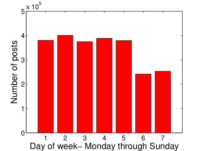
Traffic in blogosphere is not uniform; therefore, we consider traffic patterns when analyzing influence in the temporal sense. As Figure 3 illustrates, there is a seven-day periodicity. Further exploring the weekly patterns, Figure 4 shows the number of posts and the number of blog-to-blog links for different days of the week, aggregated over the entire dataset. Posting and blog-to-blog linking patterns tend to have a weekend effect of sharply dropping off at weekends.
 |
 |
| (a) Posts | (b) Blog-to-Blog links |
Next, we examine how a post’s popularity grows and declines over time. We collect all in-links to a post and plot the number of links occurring after each day following the post. This creates a curve that indicates the rise and fall of popularity. By aggregating over a large set of posts we obtain a more general pattern.
Top left plot of Figure 5 shows number of in-links for each day following a post for all posts in the dataset, while top right plot shows the in-link patterns for Monday posts only (in order to isolate the weekly periodicity). It is clear that the most links occur on the first 24 hours after the post, after that the popularity generally declines. However, in the top right plot, we note that there are “spikes” occurring every seven days, each following Monday. It almost appears as if there is compensatory behavior for the sparse weekend links. However, this is not the case. Mondays do not have an unusual number of links; Monday only appears to spike on these graphs because the natural drop-off of popularity in the following days allows Monday to tower above its followers.
 |
 |
 |
 |
 |
 |
| All posts | Only Monday posts |
Thus, fitting a general model to the drop-off graphs may be problematic, since we might obtain vastly different parameters across posts simply because they occur at different times during the week. Therefore, we smooth the in-link plots by applying a weighting parameter to the plots separated by day of week. For each delay on the horizontal axis, we estimate the corresponding day of week , and we prorate the count for by dividing it by , where is the percent of blog links occurring on day of week .
This weighting scheme normalizes the curve such that days of the week with less traffic are bumped up further to meet high traffic days, simulating a popularity drop-off that might occur if posting and linking behavior were uniform throughout the week. A smoothed version of the post drop-offs is shown in the middle row of Figure 5.
We fit the power-law distribution with a cut-off in the tail (bottom row). We fit on 30 days of data, since most posts in the graph have complete in-link patterns for the 30 days following publication. We performed the fitting over all posts and for all days of the week separately, and found a stable power-law exponent of around , which is exactly the value predicted by the model where the bursty nature of human behavior is a consequence of a decision based queuing process [4] – when individuals execute tasks based on some perceived priority, the timing of the tasks is heavy tailed, with most tasks being rapidly executed, whereas a few experience very long waiting times.
Observation 1
The probability that a post written at time acquires a link at time is:
 |
 |
 |
| (a) | (b) | (c) |
5.2 Blog network topology
The first graph we consider is the Blog network. As illustrated in Figure 1(c), every node represents a blog and there is a weighted directed edge between blogs and , where the weight of the edge corresponds to the number of posts from blog linking to posts at blog . The network contains nodes and edges. The sum of all edge weights is the number of all post to post links (). Connectivity-wise, half of the blogs belong to the largest connected component and the other half are isolated blogs.
We show the in- and out-degree distribution in Figure 6. Notice they both follow a heavy-tailed distribution. The in-degree distribution has a very shallow power-law exponent of , which suggests strong rich-get-richer phenomena. One would expect that popular active blogs that receive lots of in-links also sprout many out-links. Intuitively, the attention (number of in-links) a blog gets should be correlated with its activity (number of out-links). This does not seem to be the case. The correlation coefficient between blog’s number of in- and out-links is only , and the scatter plot in Figure 6 suggests the same.
 |
 |
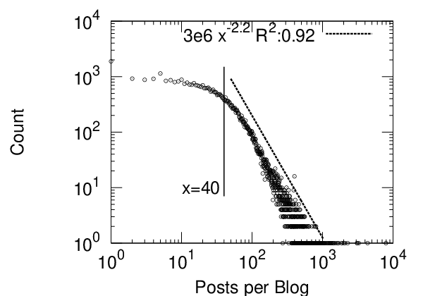
The number of posts per blog, as shown in Figure 7(a), follows a heavy-tailed distribution. The deficit of blogs with low number of posts and the knee at around 40 posts per blog can be explained by the fact that we are using a dataset biased towards active blogs. However, our biased sample of the blogs still maintains the power law in the number of blog-to-blog links (edge weights of the Blog network) as shown in 7(b). The power-law exponent is .
 |
 |
 |
 |
 |
 |
 |
 |
 |
 |
 |
 |
 |
 |
 |
 |
 |
 |
 |
 |
 |
 |
 |
 |
5.3 Post network topology
In contrast to Blog network the Post network is very sparsely connected. It contains 2.2 million nodes and only edges. of the posts are isolated, and the largest connected component accounts for nodes, while the second largest has only 153 nodes. Figure 8 shows the in- and out-degree distributions of the Post network which follow a power law with exponents and , respectively.
5.4 Patterns in the cascades
We continue with the analysis of the topological aspects of the information cascades formed when certain posts become popular and are linked by the other posts. We are especially interested in how this process propagates, how large are the cascades it forms, and as it will be shown later, what are the models that mimic cascading behavior and produce realistic cascades.
Cascades are subgraphs of the Post network that have a single root post, are time increasing (source links an existing post), and present the propagation of the information from the root to the rest of the cascade.
Given the Post network we extracted all information cascades using the following procedure. We found all cascade initiator nodes, i.e. nodes that have zero out-degree, and started following their in-links. This process gives us a directed acyclic graph with a single root node. As illustrated in Figure 2 it can happen that two cascades merge, e.g. a post gives a summary of multiple conversations (cascades). For cascades that overlap our cascade extraction procedure will extract the nodes bellow the connector node multiple times (since they belong to multiple cascades). To obtain the examples of the common shapes and count their frequency we used the algorithms as described in [17].
5.4.1 Common cascade shapes
First, we give examples of common Post network cascade shapes in Figure 9. A node represents a post and the influence flows from the top to the bottom. The top post was written first, other posts linking to it, and the process propagates. Graphs are ordered by frequency and the subscript of the label gives frequency rank. Thus, is most frequent cascade with 11 occurrences.
We find the total of cascades, and 97% of them are trivial cascades (isolated posts), 1.8% are smallest non-trivial cascades (), and the remaining 1.2% of the cascades are topologically more complex.
Most cascades can essentially be constructed from instances of stars and trees, which can model more complicated behavior like that shown in Figure 9. Cascades tend to be wide, and not too deep. Structure , which we call a cite-all chain, is especially interesting. Each post in a chain refers to every post before it in the chain.
We also find that the cascades found in the graph tend to take certain shapes preferentially. Also notice that cascade frequency rank does not simply decrease as a function of the cascade size. For example, as shown on Figure 9, a 4-star () is more common than a chain of 3 nodes (). In general stars and shallow bursty cascades are the most common type of cascades.
5.4.2 Cascade topological properties
What is the common topological pattern in the cascades? We next examine the general cascade behavior by measuring and characterizing the properties of real cascades.
 |
 |
 |
| (a) Out-degree | (b) In-degree | (c) In-degree at level |
First we observe the degree distributions of the cascades. This means that from the Post network we extract all the cascades and measure the overall degree distribution. Essentially we work with a bag of cascades, where we treat a cascade as separate disconnected sub-graph in a large network.
Figure 10(a) plots the out-degree distribution of the bag of cascades. Notice the cascade out-degree distribution is truncated, which is the result of not perfect link extraction algorithm and the upper bound on the post out-degree (500).
Figure 10(b) shows the in-degree distribution of the bag of cascades, and (c) plots the in-degree distribution of nodes at level of the cascade. A node is at level if it is hops away from the root (cascade initiator) node. Notice that the in-degree exponent is stable and does not change much given the level in the cascade. This means that posts still attract attention (get linked) even if they are somewhat late in the cascade and appear towards the bottom of it.
 |
 |
 |
| (a) All cascades | (b) Star cascade | (c) Chain cascade |
Next, we ask what distribution do cascade sizes follow? Does the probability of observing a cascade on nodes decreases exponentially with ? We examine the Cascade Size Distributions over the bag of cascades extracted from the Post network. We consider three different distributions: over all cascade size distribution, and separate size distributions of star and chain cascades. We chose stars and chains since they are well defined, and given the number of nodes in the cascade, there is no ambiguity in the topology of a star or a chain.
Figure 11 gives the Cascade Size Distribution plots. Notice all follow a heavy-tailed distribution. We fit a power-law distribution and observe that overall cascade size distribution has power-law exponent of (Figure 11(a)), stars have (Figure 11(b)), and chains are small and rare and decay with exponent (Fig. 11(c)). Also notice there are outlier chains (Fig. 11(c)) that are longer than expected. We attribute this to possible flame wars between the blogs, where authors publish posts and always refer to the last post of the other author. This creates chains longer than expected.
Observation 2
Probability of observing a cascade on nodes follows a Zipf distribution:
As suggested by Figure 9 most cascades follow tree-like shapes. To further verify this we examine how the diameter, defined as the length of the longest undirected path in the cascade, and the relation between the number of nodes and the number of edges in the cascade change with the cascade size in Figure 12.
 |
 |
| (a) Edges vs. nodes | (b) Diameter |
This gives further evidence that the cascades are mostly tree-like. We plot the number of nodes in the cascade vs. the number of edges in the cascade in Figure 12(a). Notice the number of edges in the cascade increases almost linearly with the number of nodes (). This suggests that the average degree in the cascade remains constant as the cascade grows, which is a property of trees and stars. Next, we also measure cascade diameter vs. cascade size (Figure 12(b)). We plot on linear-log scales and fit a logarithmic function. Notice the diameter increases logarithmically with the size of the cascade, which means the cascade needs to grow exponentially to gain linear increase in diameter, which is again a property of the balanced trees and very sparse graphs.
5.4.3 Collisions of cascades
By the definition we adopt in this paper, the cascade has a single initiator node, but in real life one would also expect that cascades collide and merge. There are connector nodes which are the first to bring together separate cascades. As the cascades merge, all the nodes bellow the connector node now belong to multiple cascades. We measure the distribution over the connector nodes and the nodes that belong to multiple cascades.
First, we consider only the connector nodes and plot the distribution over how many cascades a connector joins (Figure 13(a)). We only consider nodes with out-degree greater than 1, since nodes with out-degree 1 are trivial connectors – they are connecting the cascade they belong to. But there are still posts that have out-degree greater than 1, and connect only one cascade. These are the posts that point multiple out-links inside the same cascade (e.g. and of Figure 9). The dip the at the number of joined cascades equal to 1 in Figure 13(a) gives the number of such nodes.
As cascades merge, all the nodes that follow belong to multiple cascades. Figure 13(b) gives the distribution over the number of cascades a node belongs to. Here we consider all the nodes and find out that of all nodes belong to a single cascade, and the rest of distribution follows a power-law with exponent .
 |
 |
6 Proposed model and insights
What is the underlying hidden process that generates cascades? Our goal here is to find a generative model that generates cascades with properties observed in section 5.4 (Figures 10 and 11). We aim for simple and intuitive model with the least possible number of parameters.
6.1 Cascade generation model
We present a conceptual model for generating information cascades that produces cascade graphs matching several properties of real cascades. Our model is intuitive and requires only a single parameter that corresponds to how interesting (easy spreading) are the conversations in general on the blogosphere.
Intuitively, cascades are generated by the following principle. A post is posted at some blog, other bloggers read the post, some create new posts, and link the source post. This process continues and creates a cascade. One can think of cascades being a graph created by the spread of the virus over the Blog network. This means that the initial post corresponds to infecting a blog. As the cascade unveils, the virus (information) spreads over the network and leaves a trail. To model this process we use a single parameter that measures how infectious are the posts on the blogosphere. Our model is very similar to the SIS (susceptible – infected – susceptible) model from the epidemiology [13].
Next, we describe the model. Each blog is in one of two states: infected or susceptible. If a blog is in the infected state this means that the blogger just posted a post, and the blog now has a chance to spread its influence. Only blogs in the susceptible (not infected) state can get infected. When a blog successfully infects another blog, a new node is added to the cascade, and an edge is created between the node and the source of infection. The source immediately recovers, i.e. a node remains in the infected state only for one time step. This gives the model ability to infect a blog multiple times, which corresponds to multiple posts from the blog participating in the same cascade.
More precisely, a single cascade of the Cascade generation model is generated by the following process.
- (i)
Uniformly at random pick blog in the Blog network as a starting point of the cascade, set its state to infected, and add a new node to the cascade graph.
- (ii)
Blog that is now in infected state, infects each of its uninfected directed neighbors in the Blog network independently with probability . Let denote the set of infected neighbors.
- (iii)
Add new nodes to the cascade and link them to node in the cascade.
- (iv)
Set state of node to not infected. Continue recursively with step (ii) until no nodes are infected.
We make a few observations about the proposed model. First, note that the blog immediately recovers and thus can get infected multiple times. Every time a blog gets infected a new node is added to the cascade. This accounts for multiple posts from the blog participating in the same cascade. Second, we note that in this version of the model we do not try to account for topics or model the influence of particular blogs. We assume that all blogs and all conversations have the same value of the parameter . Third, the process as describe above generates cascades that are trees. This is not big limitation since we observed that most of the cascades are trees or tree-like. In the spirit of our notion of cascade we assume that cascades have a single starting point, and do not model for the collisions of the cascades.
6.2 Validation of the model
We validate our model by extensive numerical simulations. We compare the obtained cascades towards the real cascades extracted from the Post network. We find that the model matches the cascade size and degree distributions.
We use the real Blog network over which we propagate the cascades. Using the Cascade generation model we also generate the same number of cascades as we found in Post network ( million). We tried several values of parameter, and at the end decided to use . This means that the probability of cascade spreading from the infected to an uninfected blog is . We simulated our model 10 times, each time with a different random seed, and report the average.
 |
 |
 |
 |
 |
 |
 |
 |
 |
First, we show the top 10 most frequent cascades (ordered by frequency rank) as generated by the Cascade generation model in Figure 14. Comparing them to most frequent cascades from Figure 9 we notice that top 7 cascades are matched exactly (with an exception of ranks of and swapped), and rest of cascades can also be found in real data.
Next, we show the results on matching the cascade size and degree distributions in Figure 15. We plot the true distributions of the cascades extracted from the Post network with dots, and the results of our model are plotted with a dashed line. We compare four properties of cascades: (a) overall cascade size distribution, (b) size distribution of chain cascades, (c) size distribution of stars, and (d) in-degree distribution over all cascades.
Notice a very good agreement between the reality and simulated cascades in all plots. The distribution over of cascade sizes is matched best. Chains and stars are slightly under-represented, especially in the tail of the distribution where the variance is high. The in-degree distribution is also matched nicely, with an exception of a spike that can be attributed to a set of outlier blogs all with in-degree 52. Note that cascades generated by the Cascade generation model are all trees, and thus the out-degree for every node is 1.
 |
 |
| (a) All cascades | (b) Chain cascades |
 |
 |
| (c) Star cascades | (d) In-degree distribution |
6.3 Variations of the model
We also experimented with other, more sophisticated versions of the model. Namely, we investigated various strategies of selecting a starting point of the cascade, and using edge weights (number of blog-to-blog links) to further boost cascades.
We considered selecting a cascade starting blog based on the blog in-degree, in-weight or the number of posts. We experimented variants where the probability of propagating via a link is not constant but also depends on the weight of the link (number of references between the blogs). We also considered versions of the model where the probability exponentially decays as the cascade spreads away from the origin.
We found out that choosing a cascade starting blog in a biased way results in too large cascades and non-heavy tailed distributions of cascade sizes. Intuitively, this can be explained by the fact that popular blogs are in the core of the Blog network, and it is very easy to create large cascades when starting in the core. A similar problem arises when scaling with the edge weight. This can also be explained by the fact that we are not considering specific topics and associate each edge with a topic (some blog-to-blog edges may be very topic-specific) and thus we allow the cascade to spread over all edges regardless of the particular reason (the topic) that the edge between the blogs exists. This is especially true for blogs like BoingBoing 11 1 www.boingboing.net that are very general and just a collection of “wonderful things”.
7 Discussion
Our finding that the the popularity of posts drops off with a power law distribution is interesting since intuition might lead one to believe that people would “forget” a post topic in an exponential pattern. However, since linking patterns are based on the behaviors of individuals over several instances, much like other real-world patterns that follow power laws such as traffic to Web pages and scientists’ response times to letters [19], it is reasonable to believe that a high number of individuals link posts quickly, and later linkers fall off with a heavy-tailed pattern.
Our findings have potential applications in many areas. One could argue that the conversation mass metric, defined as the total number of posts in all conversation trees below the point in which the blogger contributed, summed over all conversation trees in which the blogger appears, is a better proxy for measuring influence. This metric captures the mass of the total conversation generated by a blogger, while number of in-links captures only direct responses to the blogger’s posts.
For example, we found that BoingBoing, which a very popular blog about amusing things, is engaged in many cascades. Actually, 85% of all BoingBoing posts were cascade initiators. The cascades generally did not spread very far but were wide (e.g., and in Fig. 9). On the other hand of posts from a political blog MichelleMalkin 22 2 www.michellemalkin.com were cascade initiators. But the cascade here were deeper and generally larger (e.g., in Fig. 9) than those of BoingBoing.
8 Conclusion
We analyzed one of the largest available collections of blog information, trying to find how blogs behave and how information propagates through the blogosphere. We studied two structures, the “Blog network” and the “Post network”. Our contributions are two-fold: (a) The discovery of a wealth of temporal and topological patterns and (b) the development of a generative model that mimics the behavior of real cascades. In more detail, our findings are summarized as follows:
- •
Temporal Patterns: The decline of a post’s popularity follows a power law. The slope is -1.5, the slope predicted by a very recent theory of heavy tails in human behavior [4]
- •
Topological Patterns: Almost any metric we examined follows a power law: size of cascades, size of blogs, in- and out-degrees. To our surprise, the number of in- and out-links of a blog are not correlated. Finally, stars and chains are basic components of cascades, with stars being more common.
- •
Generative model: Our idea is to reverse-engineer the underlying social network of blog-owners, and to treat the influence propagation between blog-posts as a flu-like virus, that is, the SIS model in epidemiology. Despite its simplicity, our model generates cascades that match very well the real cascades with respect to in-degree distribution, cascade size distribution, and popular cascade shapes.
Future research could try to include the content of the posts, to help us find even more accurate patterns of influence propagation. Another direction is to spot anomalies and link-spam attempts, by noticing deviations from our patterns.
Acknowledgements
This material is based upon work supported by the National Science Foundation under Grants No. SENSOR-0329549 medium ITR IIS-0534205 and under the auspices of the U.S. Department of Energy by University of California Lawrence Livermore National Laboratory under contract No.W-7405-ENG-48. This work is also partially supported by the Pennsylvania Infrastructure Technology Alliance (PITA), an IBM Faculty Award, a Yahoo Research Alliance Gift, with additional funding from Intel and NTT. Additional funding was provided by a generous gift from Hewlett-Packard. Jure Leskovec was partially supported by a Microsoft Research Graduate Fellowship, and Mary McGlohon by a National Science Foundation Graduate Fellowship.
Any opinions, findings, and conclusions or recommendations expressed in this material are those of the author(s) and do not necessarily reflect the views of the National Science Foundation, or other funding parties.
References
- [1] L. A. Adamic and N. Glance. The political blogosphere and the 2004 u.s. election: divided they blog. In LinkKDD ’05: Proceedings of the 3rd international workshop on Link discovery, pages 36–43, 2005.
- [2] E. Adar and L. A. Adamic. Tracking information epidemics in blogspace., 2005.
- [3] N. Bailey. The Mathematical Theory of Infectious Diseases and its Applications. Griffin, London, 1975.
- [4] A.-L. Barabasi. The origin of bursts and heavy tails in human dynamics. Nature, 435:207, 2005.
- [5] S. Bikhchandani, D. Hirshleifer, and I. Welch. A theory of fads, fashion, custom, and cultural change in informational cascades. Journal of Political Economy, 100(5):992–1026, October 1992.
- [6] M. Crovella and A. Bestavros. Self-similarity in world wide web traffic, evidence and possible causes. Sigmetrics, pages 160–169, 1996.
- [7] V. M. Equiluz and K. Klemm. Epidemic threshold in structured scale-free networks. arXiv:cond-mat/02055439, May 21 2002.
- [8] M. Faloutsos, P. Faloutsos, and C. Faloutsos. On power-law relationships of the internet topology. In SIGCOMM, pages 251–262, 1999.
- [9] N. S. Glance, M. Hurst, K. Nigam, M. Siegler, R. Stockton, and T. Tomokiyo. Deriving marketing intelligence from online discussion. In KDD, 2005.
- [10] J. Goldenberg, B. Libai, and E. Muller. Talk of the network: A complex systems look at the underlying process of word-of-mouth. Marketing Letters, 2001.
- [11] M. Granovetter. Threshold models of collective behavior. Am. Journal of Sociology, 83(6):1420–1443, 1978.
- [12] D. Gruhl, R. Guha, D. Liben-Nowell, and A. Tomkins. Information diffusion through blogspace. In WWW ’04, 2004.
- [13] H. W. Hethcote. The mathematics of infectious diseases. SIAM Rev., 42(4):599–653, 2000.
- [14] D. Kempe, J. Kleinberg, and E. Tardos. Maximizing the spread of influence through a social network. In KDD ’03, 2003.
- [15] R. Kumar, J. Novak, P. Raghavan, and A. Tomkins. On the bursty evolution of blogspace. In WWW ’03, pages 568–576. ACM Press, 2003.
- [16] J. Leskovec, L. A. Adamic, and B. A. Huberman. The dynamics of viral marketing. In EC ’06: Proceedings of the 7th ACM conference on Electronic commerce, pages 228–237, New York, NY, USA, 2006. ACM Press.
- [17] J. Leskovec, A. Singh, and J. Kleinberg. Patterns of influence in a recommendation network. In Pacific-Asia Conference on Knowledge Discovery and Data Mining (PAKDD), 2006.
- [18] M. Richardson and P. Domingos. Mining knowledge-sharing sites for viral marketing, 2002.
- [19] A. Vazquez, J. G. Oliveira, Z. Dezso, K. I. Goh, I. Kondor, and A. L. Barabasi. Modeling bursts and heavy tails in human dynamics. Physical Review E, 73:036127, 2006.
- [20] M. Wang, T. Madhyastha, N. H. Chang, S. Papadimitriou, and C. Faloutsos. Data mining meets performance evaluation: Fast algorithms for modeling bursty traffic. ICDE, Feb. 2002.
- [21] Y. Wang, D. Chakrabarti, C. Wang, and C. Faloutsos. Epidemic spreading in real networks: An eigenvalue viewpoint. In SRDS, pages 25–34, 2003.
- [22] D. J. Watts. A simple model of global cascades on random networks. In PNAS, 2002.
- [23] G. Zipf. Human Behavior and Principle of Least Effort: An Introduction to Human Ecology. Addison Wesley, Cambridge, Massachusetts, 1949.