On-Shell Methods in Perturbative QCD

The first hint that this approach might be useful comes from investigating three-point helicity amplitudes [82], displayed in fig. 1(a). For real momenta, an on-shell process with three external massless legs $i,j,k$ is always singular, because $s_{ij}=0$ for all three pairs of legs. These conditions force the three momenta to be collinear with each other — if they are real — which in turn makes all kinematic quantities vanish. Using complex momenta to define the amplitude for three massless particles is also not a new idea. For example, Goroff and Sagnotti [84] used complex momenta to define non-singular three-graviton kinematics, in their on-shell computation of the two-loop divergence in pure Einstein gravity. However, there is a natural way to take the kinematics to be complex using spinor variables, which meshes neatly with the structure of helicity amplitudes.

First we introduce a shorthand notation for the two-component (Weyl) spinors associated with an $n$-parton process [82]:

It is also convenient to describe the spinors with a ‘bra’ and ‘ket’ notation,

One can always reconstruct the momenta from the spinors, using the positive-energy projector for massless spinors, $u(k)\bar{u}(k)={\raise 0.97221pt\hbox to5.52084pt{\hss/\hss}\hbox to0.0pt{\hss$k$}}$, or

Equation (2.3) shows that a massless momentum vector, written as a bi-spinor, is simply the product of a left-handed spinor with a right-handed one. This result is also valid for complex momenta.

Lorentz-invariant spinor products can be defined using the antisymmetric tensors $\varepsilon^{\alpha\beta}$ and $\varepsilon^{\dot{\alpha}\dot{\beta}}$ for the $SU(2)$ factors in the Lorentz algebra, $SL(2,R)\sim SU(2)_{L}\times SU(2)_{R}$:

(The sign of $\left[j\,l\right]$ in eq. (2.5) matches that in most of the QCD literature; in much of the ‘twistor’ literature, e.g. refs. [82, 49, 8, 9], the opposite sign is used.) These products are antisymmetric, $\left\langle j\,l\right\rangle=-\left\langle l\,j\right\rangle$, $\left[j\,l\right]=-\left[l\,j\right]$. The usual momentum dot products can be constructed from the spinor products using the relation,

We will also use the notation

where the sums run over cyclically ordered labels between $r$ and $s$, as well as,

Parity acts on a helicity amplitude by flipping the sign of all helicities. This symmetry may be implemented by exchanging the left- and right-handed spinor products in the amplitude, $\left\langle j\,l\right\rangle\leftrightarrow\left[l\,j\right]$.

For real momenta, $\lambda_{i}$ and ${\tilde{\lambda}}_{i}$ are complex conjugates of each other. Therefore the spinor products are complex square roots of the Lorentz products,

In this case, if all the $s_{jl}$ vanish, then so do all the spinor products. However, for complex momenta, eq. (2.10) does not hold. In fact, it is possible to choose all three left-handed spinors to be proportional, ${\tilde{\lambda}}_{1}=c_{1}{\tilde{\lambda}}_{3}$, ${\tilde{\lambda}}_{2}=c_{2}{\tilde{\lambda}}_{3}$, while the right-handed spinors are not proportional, but obey the relation, $c_{1}\lambda_{1}+c_{2}\lambda_{2}+\lambda_{3}=0$, which follows from momentum conservation, $k_{1}+k_{2}+k_{3}=0$, and eq. (2.3). Then

while $\left\langle 1\,2\right\rangle$, $\left\langle 2\,3\right\rangle$ and $\left\langle 3\,1\right\rangle$ are all nonvanishing.

For this kinematical choice, the tree-level primitive amplitude for two negative helicities and one positive helicity, $A_{3}^{\rm tree}$, is nonsingular, even though all momentum invariants $s_{jl}$ vanish according to eq. (2.6). (We assign helicities to particles under the assumption that they are outgoing; if a particle is incoming, its true helicity is opposite to the label.) For three gluons, $A_{3}^{\rm tree}$ can be evaluated using the three-gluon-vertex in the color-ordered Feynman rules [71], as

In the spinor-helicity formalism [77, 78], the polarization vectors $\varepsilon_{i}^{\pm}$ are expressed as,

in terms of null reference momenta $q_{i}$, which may be chosen to simplify the computation. In eq. (2.12), if we choose $q_{2}=q_{1}$ and $q_{3}=k_{1}$, then $\varepsilon_{1}^{-}\cdot\varepsilon_{2}^{-}=\varepsilon_{3}^{+}\cdot\varepsilon_{1}^{-}=0$. Upon using a Fierz rearrangement and momentum conservation, the lone surviving term in eq. (2.12) becomes,

or

Equation (2.15) is the first member of the sequence of Parke-Taylor, or maximally-helicity-violating (MHV), tree amplitudes for $n$ gluons [85, 86, 87],

In this expression, only gluons $j$ and $k$ have negative helicity; the remaining $(n-2)$ gluons have positive helicity. For $n\geq 4$, these amplitudes are well-defined for real momenta. However, for $n=3$, formula (2.15) only makes sense for complex momenta of the type (2.11).

There is a class of complex momenta conjugate to eq. (2.11), for which

while $\left[1\,2\right]$, $\left[2\,3\right]$ and $\left[3\,1\right]$ are all nonvanishing. Such momenta make the parity-conjugate three-point amplitude,

well-defined. When the amplitude $A_{3}^{\rm tree}(1^{-},2^{-},3^{+})$ appears in the ‘wrong’ kinematics (2.17), it should be set to zero, because more vanishing spinor products appear in the numerator than in the denominator.

For any on-shell complex momenta, the all-positive amplitude vanishes,

This result follows easily by choosing all reference momenta $q_{i}$ to be the same, which forces $\varepsilon_{i}^{+}\cdot\varepsilon_{j}^{+}$ to vanish for all pairs $i,j$. The same result holds for $A_{3}^{\rm tree}(1^{-},2^{-},3^{-})$, of course. In a similar fashion, the three-point amplitude for a pair of massless quarks (which must carry opposite helicity) plus one gluon is well-defined and nonzero using the kinematics (2.11) if the gluon helicity is negative, and using the kinematics (2.17) if it is positive. It vanishes for the ‘wrong’ kinematics. These rules will become important later for evaluating generalized unitarity cuts and recursive diagrams containing three-point vertices.

We have seen how suitable complex kinematics can simplify the structure of the three-point amplitude. Much more significantly, however, complex kinematics allow the exploration of generic factorization singularities of on-shell amplitudes, and the use of factorization information to reconstruct the amplitude, as was recognized at tree-level by Britto, Cachazo, Feng and Witten (BCFW) [9]. We will review the BCFW recursion relations in the next section. Here we shall just discuss the simple example of the Parke-Taylor amplitudes. The idea is to embed a tree amplitude $A_{n}^{\rm tree}$ into a one-complex-parameter family of on-shell amplitudes $A_{n}^{\rm tree}(z)$. The rationale for introducing the complex parameter $z$ is that it allows us to apply the full power of complex variable theory to reconstruct amplitudes from their poles. The simplest way to introduce this parameter is by modifying, or ‘shifting’ the momenta of just two of the $n$ partons, in a way that keeps them on shell. Because of eq. (2.3), the two momenta will automatically remain on shell if we shift the spinor variables, and then define the shifted momenta to be the products of the new left- and right-handed spinors.

We define the ${[j,l\rangle}$ shift to be [9],

where $z$ is a complex parameter. The shift leaves untouched $\lambda_{j}$, ${\tilde{\lambda}}_{l}$, and the spinors for all the other particles in the process. Under the shift, the corresponding momenta shift as,

which preserves their masslessness, $k_{j}^{2}(z)=0=k_{l}^{2}(z)$, as well as overall momentum conservation.

Suppose we apply the ${[n,1\rangle}$ shift, ${\tilde{\lambda}}_{n}\rightarrow{\tilde{\lambda}}_{n}-z{\tilde{\lambda}}_{1}$, $\lambda_{1}\rightarrow\lambda_{1}+z\lambda_{n}$, to the MHV amplitude (2.16), for the case $k=n$ (and $j\neq 1$). Because the formula contains only right-handed $\lambda_{i}$ spinors, the only induced $z$ dependence arises from terms containing $\lambda_{1}$. The spinor product $\left\langle 1\,2\right\rangle$ is shifted to $\left\langle 1\,2\right\rangle\to\left\langle 1\,2\right\rangle+z\left\langle n\,2\right\rangle$ The spinor product $\left\langle n\,1\right\rangle$ is unaffected, because $\left\langle n\,1\right\rangle\to\left\langle n\,1\right\rangle+z\left\langle n\,n\right\rangle$, but $\left\langle n\,n\right\rangle=0$ by antisymmetry. Thus the MHV amplitude becomes

If we divide this shifted amplitude by $z$, we get a function with two poles at finite $z$, one at the origin and one at $z=-\left\langle 1\,2\right\rangle/\left\langle n\,2\right\rangle$, as shown in fig. 2. The function behaves like $1/z^{2}$ as $z\to\infty$, so the integral around the circle $C$ at infinity vanishes,

Cauchy’s theorem then guarantees that the two poles at finite $z$ have equal and opposite residue.

The residue of the pole at the origin is simply the MHV amplitude we want to compute, $A_{n}^{{\rm tree\,MHV},\,jn}(0)=A_{n}^{{\rm tree\,MHV},\,jn}\equiv A_{n}$. The residue of the second pole is determined by the factorization properties of the amplitude, because it occurs at the point that the intermediate momentum $K_{12}(z)\ \equiv\ k_{1}(z)+k_{2}$ goes on shell, $K_{12}^{2}(z)=(\left\langle 1\,2\right\rangle+z\left\langle n\,2\right\rangle)\left[2\,1\right]\ \to\ 0$. That is, at the value $z=z_{12}\equiv-\left\langle 1\,2\right\rangle/\left\langle n\,2\right\rangle$ we have,

A hat on a kinematic variable means that a shift of the form (2.20) has been applied to the variable, with $z$ then fixed to the value that puts an intermediate momentum on shell. The key point is that, because an intermediate state goes on shell, the amplitude factorizes at this point into the product of two lower-point amplitudes, multiplied by the diverging propagator. In general there is a sum over the helicity $h$ of the intermediate state, $h=\pm 1$ for intermediate gluons.

Equating the residue at $z=z_{12}$ to the negative of the one at the origin, we have

In the second step we evaluated the residue in brackets, and used the vanishing of $A_{3}^{\rm tree}(1^{+},2^{+},3^{+})$ in eq. (2.19) to reduce the helicity sum to a single term.

Equation (2.25) is the prototype for the tree-level BCFW recursion relation reviewed in section 3. In general, there will be several terms on the right-hand side, corresponding to different nontrivial factorization channels which can be probed for suitable values of $z$. The MHV amplitudes are unique in having no multi-particle poles, which is related to the vanishing of $n$-gluon amplitudes with fewer negative helicities,

For this reason, the recursion relation (2.25) in the MHV case has but a single term.

We can further evaluate eq. (2.25) using the explicit form (2.16) of the MHV amplitudes, as a simple exercise in manipulating the hatted variables that appear, and as an on-shell recursive proof of the formula. (As an historical note, the first proof of eq. (2.16) employed recursion relations of the off-shell variety [6].) Inserting the forms of the $(n-1)$-point and three-point amplitudes, eq. (2.25) becomes,

We need to continue the spinors for $(-{\hat{K}}_{12})$ into those for ${\hat{K}}_{12}$. Because a pair of such spinors appears, we pick up a minus sign. (Determining the sign for the case of an intermediate quark line is more subtle.)

Because the ${[n,1\rangle}$ shift leaves ${\tilde{\lambda}}_{1}$ and $\lambda_{n}$ alone, we can let $\hat{n}\rangle\to n\rangle$ and $\hat{1}]\to 1]$ in eq. (2.27). Because the shifted momentum is proportional to ${\tilde{\lambda}}_{1}\lambda_{n}$, a hatted momentum appearing in a right-handed spinor product with $n$, or in a left-handed spinor product with $1$, can have its hat removed as well. For this reason, it is very convenient to use factors of $\left\langle\smash{n}\,\smash{{\hat{K}}_{12}}\right\rangle$ and $\left[\smash{{\hat{K}}_{12}}\,\smash{1}\right]$ to clean up other spinor products containing ${\hat{K}}_{12}$, inserting them into the numerator and denominator of expressions as needed. In the present case, the necessary factors are already present. Equation (2.27) becomes,

The final form indeed matches the expression (2.16), thus confirming it recursively.

Figure 1(b) shows a second class of configurations for which complex kinematics are useful, namely generalized unitarity conditions, which will be discussed in more detail in section 4. At one loop, conventional unitarity constraints on amplitudes are analyzed by putting two intermediate states on shell. For example, if legs 1, 2, 3 and 4 in fig. 1(b) are outgoing, and legs 5, 6, 7 and 8 are incoming, then the conventional cut in the 1234 channel is computed by imposing $\ell_{1}^{2}=\ell_{5}^{2}=0$. This constraint can be realized with all momenta real in Minkowski space. It can then be interpreted as a $4\to 2$ particle scattering process, followed by a $2\to 4$ particle scattering.

Generalized unitarity corresponds to requiring more than two internal particles to be on shell. Often these constraints cannot be realized with real Minkowski momenta. Suppose we try to add the condition $\ell_{3}^{2}=0$ to the standard cut constraints $\ell_{1}^{2}=\ell_{5}^{2}=0$ in fig. 1(b). The problem is that $1\to 3$ processes are forbidden for real, non-collinear massless momenta, although $2\to 2$ processes are allowed. After setting $\ell_{3}^{2}=0$, fig. 1(b) contains a four-point subamplitude in which leg $\ell_{1}$ is incoming, and legs 1 and 2 are outgoing with $s_{12}$ nonzero. We can arrange for this to be a real Minkowski process by taking $\ell_{3}$ to be incoming. But then the subamplitude below it in the figure has only leg $\ell_{5}$ incoming, and legs $\ell_{3}$, 3 and 4 outgoing. It cannot correspond to a real on-shell process, as long as $s_{34}$ is nonzero.

Similarly, we cannot impose $\ell_{7}^{2}=0$ on top of $\ell_{1}^{2}=\ell_{5}^{2}=0$, in the process $5\,+\,6\,+\,7\,+\,8\to 1\,+\,2\,+\,3\,+\,4$, and still have real momenta. Typically then, one needs to allow for complex momenta in order to implement generalized cut conditions. As an even simpler example, if we consider a quadruple cut with fewer than the eight external momenta shown in fig. 1(b), then at least one tree amplitude will have only three external legs, and this fact alone dictates complex momenta.

On the other hand, generalized cut conditions can sometimes be satisfied with only real momenta. In fig. 1(b), suppose now that the scattering process has legs 4, 5, 6 and 7 incoming, and legs 8, 1, 2 and 3 outgoing. Then it is possible to solve all four internal constraints, $\ell_{1}^{2}=\ell_{3}^{2}=\ell_{5}^{2}=\ell_{7}^{2}=0$, with real Minkowski momenta, corresponding to scattering that proceeds from the lower left to the upper right of the figure; that is, $5\,+\,6\to\ell_{7}\,+\,\ell_{5}$, followed by $\ell_{7}\,+\,7\to 8\,+\,\ell_{1}$ and $4\,+\,\ell_{5}\to\ell_{3}\,+\,3$, followed by $\ell_{3}\,+\,\ell_{1}\to 1\,+\,2$.

In this section we describe the construction of tree amplitudes via on-shell recursion. As alluded to in the previous section, the BCFW recursion relation [8, 9] is based on introducing a complex-parameter-dependent shift of two of the external massless spinors, as given in eq. (2.20). The construction of tree amplitudes via on-shell recursion essentially amounts to generalizing and reversing the steps in section 2.2. Instead of starting with a known amplitude, and verifying its analytic properties under the parameter-dependent shift, we use such properties to systematically construct unknown amplitudes.

Following the same procedure as for the MHV case in eq. (2.22), for generic amplitudes we define an analytically continued amplitude,

which remains on-shell, but depends on the complex parameter $z$. If $A$ is a tree amplitude, then $A(z)$ is a rational function of $z$. The physical amplitude is given by $A(0)$.

Following the MHV case (2.23) consider the contour integral,

where the contour is taken around the circle at infinity. If $A(z)\rightarrow 0$ as $z\rightarrow\infty$, the contour integral vanishes and we obtain a relationship between the physical amplitude, at $z=0$, and a sum over residues for the poles of $A(z)$, located at $z_{\alpha}$,

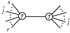
To determine the residues at each pole, we use the general factorization properties that any amplitude must satisfy as an intermediate momentum $K^{\mu}$ goes on shell, $K^{2}\to 0$. In general, the residue is given by a product of lower-point on-shell amplitudes. Only a subset of the possible factorization limits for an amplitude are explored by the $z$-dependent shift. Poles in the $z$ plane can develop in any channel that has leg $j$ on one side of the pole and leg $l$ on the other side, because the intermediate momentum is $z$-dependent. Thus we can solve the on-shell condition,

The solution is

A contribution to the recursion relation from this residue is illustrated diagrammatically in fig. 3. To get the precise form of the contribution, using eq. (3.3), we need to evaluate the residue (as we did in eq. (2.25) for a special case),

The final form of the tree-level recursion relation is [8, 9]

Generically we have a double sum, labeled by $r,s$, over recursive diagrams, with legs $j$ and $l$ always appearing on opposite sides of the pole. There is also a sum over the helicity $h$ of the intermediate state. The squared momentum associated with the pole, $K_{r\cdots s}^{2}$, arising from eq. (3.6), is evaluated in the unshifted kinematics. The on-shell tree amplitudes $A_{L}$ and $A_{R}$ are evaluated in kinematics that have been shifted by eq. (2.20), with $z=z_{rs}$. The shifted momenta for such kinematics are indicated by hats.

Equation (3.7) may alternatively be derived by expressing $A(z)$ as a sum over poles multiplied by their residues (under our assumption that $A(z)\rightarrow 0$ as $z\rightarrow\infty$). This representation, valid for all $z$, is

By setting $z=0$ in this formula, we recover the recursion relation (3.7).

To derive the recursion relation, we assumed that the amplitude $A(z)$ vanishes as $z\to\infty$. If all the external particles are gluons, then the validity of this assumption depends only on the helicity of the two shifted legs. There are four different cases, which we can label by ${[h_{j},h_{l}\rangle}={[\pm,\pm\rangle}$. A shift of type ${[+,-\rangle}$ does not generally make $A(z)$ vanish at infinity. As an example, the MHV amplitude (2.16) behaves as either $z^{2}$ or $z^{3}$ as $z\to\infty$, because of the factor of ${\left\langle j\,k\right\rangle}^{4}$ in the numerator. The case ${[-,+\rangle}$ is the simplest to analyze because each individual Feynman diagram vanishes separately [9]. Shifts of type ${[-,-\rangle}$ and ${[+,+\rangle}$ also make the amplitude vanish as $z\rightarrow\infty$, but here cancellations between Feynman diagrams are required. The vanishing behavior has been proven using generalizations of the shift (2.20) that affect three or more momenta [88, 75].

The on-shell recursion relation (3.7) contains spinor products involving hatted momenta. For the purposes of numerical evaluation, we can leave the amplitudes in this form, because the complex hatted momenta are built from well-defined spinors, whose inner products can be computed from eqs. (2.4) and (2.5). However, for analytic purposes it is useful to eliminate the hatted momenta in favor of external momenta. We can make use of the following relations,

To simplify the expressions we used, for example,

where the last term vanishes by a Fierz identity. The product $A_{L}^{h}\times A_{R}^{-h}$ is homogeneous in the spinors carrying the intermediate momentum ${\hat{K}}_{r\cdots s}$. Because of this, any remaining factors of $\left\langle\smash{j}\,\smash{{\hat{K}}_{r\cdots s}}\right\rangle$ and $\left[\smash{{\hat{K}}_{r\cdots s}}\,\smash{l}\right]$ can be paired up to give factors of

Recursive diagrams containing three-point amplitudes often vanish because the ‘wrong’ kinematics are present. In general, if a ${[j,l\rangle}$ shift is used, and the recursive diagram contains a three-vertex with two positive helicities, one of which is $j$, then the diagram vanishes. The reason is that the spinor $\lambda_{j}$ is unaffected by the shift, so its product with the spinor for the other external leg $a$ in the three-point amplitude, $\left\langle j\,a\right\rangle$, remains nonvanishing. Therefore $\left[j\,a\right]$, and all of the left-handed spinor products, must vanish, and so the three-vertex with two positive helicities vanishes, as discussed in section 2. Similarly, three-vertices with two negative helicities can also be dropped, when one of the three legs is $l$.

As a first example, consider the amplitude $A_{4}^{\rm tree}(1^{-},2^{-},3^{+},4^{+})$. This amplitude can be constructed recursively from the three-point amplitudes given in eqs. (2.15) and (2.18). As discussed above, for the ${[1,2\rangle}$ shift (a ${[-,-\rangle}$ shift) the amplitude vanishes for large $z$. Using this shift, there are two potential terms in the recursion relation, corresponding to diagrams (a) and (b) in fig. 4.

The first of these diagrams,

vanishes because of the ‘wrong’ kinematics discussed above.

Now evaluate diagram (b), using eqs. (2.15) and (2.18), with an overall minus sign for the continuation $-{\hat{K}}_{23}\to{\hat{K}}_{23}$,

This form is already satisfactory for the purpose of evaluating the amplitude numerically. It is, however, a useful exercise to eliminate hatted momenta in favor of unhatted external momenta. Applying the substitutions (3.9) and simplifying the expression for diagram (b), we find

in agreement with the MHV formula (2.16).

Interestingly, using the on-shell recursion relations, the four-point amplitude, and indeed all tree amplitudes, can be constructed from the on-shell three-vertices. The four-point vertex in the Yang-Mills Feynman rules is unnecessary. On the other hand, the four-point vertex is related by gauge invariance to the three-point vertex. Gauge invariance is necessary to decouple unphysical states. The recursion relations rely on the fact that such states are not present in factorization limits. In this way, they implicitly incorporate the correct four-point vertex.

Consider now the less trivial example of a six-point next-to-MHV (NMHV) amplitude, $A_{6}^{\rm tree}(1^{-},2^{-},3^{-},4^{+},5^{+},6^{+})$. Using a ${[3,4\rangle}$ shift (a ${[-,+\rangle}$ shift) yields the two recursive diagrams in fig. 5,

The first of these diagrams gives,

Applying eq. (3.9), we may rewrite this expression in terms of unhatted momenta, using the definitions in eqs. (2.7) and (2.9),

Similarly, diagram (b) in fig. 5 is given by

It is interesting that this kind of representation of the amplitude is intimately connected [89] to the forms in which tree amplitudes appear in the infrared singularities of certain one-loop amplitudes [68]. This feature is related to the appearance of denominator factors such as $\left\langle\smash{5}{\vphantom{1}}^{-}\right|{K_{34}}\left|\smash{2}{\vphantom{1}}^{-}\right\rangle$ at one loop, where they arise in the reduction of various loop integrals to a basic set of integrals. They can be thought of as spinor ‘square roots’ of certain Gram determinants.

The expression $\left\langle\smash{5}{\vphantom{1}}^{-}\right|{K_{34}}\left|\smash{2}{\vphantom{1}}^{-}\right\rangle$ vanishes on a subspace of phase space. For example, when $K_{34}^{\mu}$ is any linear combination of $k_{2}^{\mu}$ and $k_{5}^{\mu}$, it vanishes using the massless Dirac equation, ${\raise 0.97221pt\hbox to5.52084pt{\hss/\hss}\hbox to0.0pt{\hss$k$}}u_{\pm}(k)=0$. Note that $\left\langle\smash{5}{\vphantom{1}}^{-}\right|{K_{34}}\left|\smash{2}{\vphantom{1}}^{-}\right\rangle=-\left\langle\smash{5}{\vphantom{1}}^{-}\right|{K_{61}}\left|\smash{2}{\vphantom{1}}^{-}\right\rangle$ by momentum conservation, and so the latter form also vanishes on the same subspace. This subspace does not correspond to physical factorizations of the amplitude, so $D_{6}^{\rm(a)}$ and $D_{6}^{\rm(b)}$ each have spurious singularities on it. However, their sum, the full amplitude $A_{6}^{\rm tree}$, is nonsingular. In principle, a numerical program should check for small values of such spurious denominator factors, in order to avoid round-off errors. (Near a spurious singularity for the above representation (3.16), one could for example make use of a different shift (2.20), whose spurious singularities are located elsewhere.) On the other hand, the singularity is fairly mild, because only one power of $\left\langle\smash{5}{\vphantom{1}}^{-}\right|{K_{34}}\left|\smash{2}{\vphantom{1}}^{-}\right\rangle$ appears in the denominator.

References

- [1] T. Stelzer and W. F. Long, Comput. Phys. Commun. 81, 357 (1994) [hep-ph/9401258].
- [2] A. Pukhov et al., hep-ph/9908288.
- [3] F. Krauss, R. Kuhn and G. Soff, JHEP 0202, 044 (2002) [hep-ph/0109036].
- [4] M. L. Mangano, M. Moretti, F. Piccinini, R. Pittau and A. D. Polosa, JHEP 0307, 001 (2003) [hep-ph/0206293].
- [5] A. Kanaki and C. G. Papadopoulos, Comput. Phys. Commun. 132, 306 (2000) [hep-ph/0002082].
- [6] F. A. Berends and W. T. Giele, Nucl. Phys. B 306, 759 (1988).
- [7]
D. A. Kosower,
Nucl. Phys. B 335, 23 (1990);
F. Caravaglios and M. Moretti, Phys. Lett. B 358, 332 (1995) [hep-ph/9507237];
P. Draggiotis, R. H. P. Kleiss and C. G. Papadopoulos, Phys. Lett. B 439, 157 (1998) [hep-ph/9807207];
F. Caravaglios, M. L. Mangano, M. Moretti and R. Pittau, Nucl. Phys. B 539, 215 (1999) [hep-ph/9807570]. - [8] R. Britto, F. Cachazo and B. Feng, Nucl. Phys. B 715, 499 (2005) [hep-th/0412308].
- [9] R. Britto, F. Cachazo, B. Feng and E. Witten, Phys. Rev. Lett. 94, 181602 (2005) [hep-th/0501052].
- [10] F. A. Berends, W. T. Giele and H. Kuijf, Nucl. Phys. B 321, 39 (1989).
- [11]
H. U. Bengtsson and T. Sjöstrand,
Comput. Phys. Commun. 46, 43 (1987);
T. Sjöstrand, P. Eden, C. Friberg, L. Lönnblad, G. Miu, S. Mrenna and E. Norrbin, Comput. Phys. Commun. 135, 238 (2001) [hep-ph/0010017]. - [12]
G. Marchesini and B. R. Webber,
Cavendish-HEP-87/9;
G. Marchesini, B. R. Webber, G. Abbiendi, I. G. Knowles, M. H. Seymour and L. Stanco, Comput. Phys. Commun. 67, 465 (1992);
G. Corcella et al., hep-ph/0210213. - [13]
S. Catani, F. Krauss, R. Kuhn and B. R. Webber,
JHEP 0111, 063 (2001)
[hep-ph/0109231];
S. Mrenna and P. Richardson, JHEP 0405, 040 (2004) [hep-ph/0312274];
M. Mangano, presented at the Fermilab ME/MC Tuning Workshop, October 4, 2004;
S. Höche, F. Krauss, N. Lavesson, L. Lönnblad, M. Mangano, A. Schälicke and S. Schumann, hep-ph/0602031;
M. L. Mangano, M. Moretti, F. Piccinini and M. Treccani, JHEP 0701, 013 (2007) [hep-ph/0611129]. - [14]
S. Catani, D. de Florian and M. Grazzini,
JHEP 0105, 025 (2001)
[hep-ph/0102227];
R. V. Harlander and W. B. Kilgore, Phys. Rev. Lett. 88, 201801 (2002) [hep-ph/0201206];
C. Anastasiou and K. Melnikov, Nucl. Phys. B 646, 220 (2002) [hep-ph/0207004];
V. Ravindran, J. Smith and W. L. van Neerven, Nucl. Phys. B 665, 325 (2003) [hep-ph/0302135]. - [15]
S. Frixione and B.R. Webber,
JHEP 0206, 029 (2002)
[hep-ph/0204244];
S. Frixione, P. Nason and B.R. Webber, JHEP 0308, 007 (2003) [hep-ph/0305252]. - [16]
P. Nason,
JHEP 0411, 040 (2004)
[hep-ph/0409146];
Z. Nagy and D. E. Soper, JHEP 0510, 024 (2005) [hep-ph/0503053];
M. Krämer, S. Mrenna and D. E. Soper, Phys. Rev. D 73, 014022 (2006) [hep-ph/0509127];
P. Nason and G. Ridolfi, JHEP 0608, 077 (2006) [hep-ph/0606275];
O. Latunde-Dada, S. Gieseke and B. Webber, JHEP 0702, 051 (2007) [hep-ph/0612281]. - [17]
Z. Kunszt and D. E. Soper,
Phys. Rev. D 46, 192 (1992);
S. Frixione, Z. Kunszt and A. Signer, Nucl. Phys. B 467, 399 (1996) [hep-ph/9512328]. - [18]
W. T. Giele and E. W. N. Glover,
Phys. Rev. D 46, 1980 (1992);
W. T. Giele, E. W. N. Glover and D. A. Kosower, Nucl. Phys. B 403, 633 (1993) [hep-ph/9302225]. - [19] S. Catani and M. H. Seymour, Phys. Lett. B 378, 287 (1996) [hep-ph/9602277]; Nucl. Phys. B 485, 291 (1997) [Erratum-ibid. B 510, 503 (1998)] [hep-ph/9605323].
- [20] S. Catani, S. Dittmaier, M. H. Seymour and Z. Trócsányi, Nucl. Phys. B 627, 189 (2002) [hep-ph/0201036].
- [21]
Phys. Rev. D 57, 5410 (1998)
[hep-ph/9710213];
J. M. Campbell, M. A. Cullen and E. W. N. Glover, Eur. Phys. J. C 9, 245 (1999) [hep-ph/9809429]. - [22] A. Gehrmann-De Ridder, T. Gehrmann and E. W. N. Glover, JHEP 0509, 056 (2005) [hep-ph/0505111].
- [23]
W. Beenakker, S. Dittmaier, M. Krämer, B. Plümper, M. Spira
and P. M. Zerwas,
Phys. Rev. Lett. 87, 201805 (2001)
[hep-ph/0107081];
Nucl. Phys. B 653, 151 (2003)
[hep-ph/0211352];
S. Dawson, L. H. Orr, L. Reina and D. Wackeroth, Phys. Rev. D 67, 071503 (2003) [hep-ph/0211438];
S. Dawson, C. Jackson, L. H. Orr, L. Reina and D. Wackeroth, Phys. Rev. D 68, 034022 (2003) [hep-ph/0305087]. - [24] W. B. Kilgore and W. T. Giele, Phys. Rev. D 55, 7183 (1997) [hep-ph/9610433]. Z. Nagy, Phys. Rev. Lett. 88, 122003 (2002) [hep-ph/0110315]; Phys. Rev. D 68, 094002 (2003) [hep-ph/0307268].
- [25]
J. Campbell and R. K. Ellis,
Phys. Rev. D 65, 113007 (2002)
[hep-ph/0202176];
J. Campbell, R. K. Ellis and D. L. Rainwater, Phys. Rev. D 68, 094021 (2003) [hep-ph/0308195]. - [26]
S. Dawson, C. B. Jackson, L. Reina and D. Wackeroth,
Mod. Phys. Lett. A 21, 89 (2006)
[hep-ph/0508293];
F. Febres Cordero, L. Reina and D. Wackeroth, Phys. Rev. D 74, 034007 (2006) [hep-ph/0606102]. - [27] J. M. Campbell, R. K. Ellis and G. Zanderighi, JHEP 0610, 028 (2006) [hep-ph/0608194].
- [28]
A. Brandenburg, S. Dittmaier, P. Uwer and S. Weinzierl,
Nucl. Phys. Proc. Suppl. 135, 71 (2004)
[hep-ph/0408137];
S. Dittmaier, P. Uwer and S. Weinzierl, hep-ph/0703120. - [29] A. Lazopoulos, K. Melnikov and F. Petriello, hep-ph/0703273.
- [30] A. I. Davydychev, Phys. Lett. B 263, 107 (1991).
- [31] A. Ferroglia, M. Passera, G. Passarino and S. Uccirati, Nucl. Phys. B 650, 162 (2003) [hep-ph/0209219].
- [32] Y. Kurihara et al., Nucl. Phys. B 654, 301 (2003) [hep-ph/0212216]; Nucl. Phys. Proc. Suppl. 157, 231 (2006).
- [33] A. Denner and S. Dittmaier, Nucl. Phys. B 658, 175 (2003) [hep-ph/0212259]; Nucl. Phys. B 734, 62 (2006) [hep-ph/0509141].
- [34] W. T. Giele and E. W. N. Glover, JHEP 0404, 029 (2004) [hep-ph/0402152].
- [35] F. del Aguila and R. Pittau, JHEP 0407, 017 (2004) [hep-ph/0404120].
- [36] R. K. Ellis, W. T. Giele and G. Zanderighi, Phys. Rev. D 72, 054018 (2005) [Erratum-ibid. D 74, 079902 (2006)] [hep-ph/0506196].
- [37] T. Binoth, J. P. Guillet, G. Heinrich, E. Pilon and C. Schubert, JHEP 0510, 015 (2005) [hep-ph/0504267].
- [38] R. K. Ellis, W. T. Giele and G. Zanderighi, Phys. Rev. D 73, 014027 (2006) [hep-ph/0508308].
- [39] R. K. Ellis, W. T. Giele and G. Zanderighi, JHEP 0605, 027 (2006) [hep-ph/0602185].
- [40] Z. Xiao, G. Yang and C. J. Zhu, Nucl. Phys. B 758, 53 (2006) [hep-ph/0607017].
- [41] T. Binoth, J. P. Guillet and G. Heinrich, JHEP 0702, 013 (2007) [hep-ph/0609054].
- [42] G. Ossola, C. G. Papadopoulos and R. Pittau, Nucl. Phys. B 763, 147 (2007) hep-ph/0609007].
- [43]
M. Krämer and D. E. Soper,
Phys. Rev. D 66, 054017 (2002)
[hep-ph/0204113];
Z. Nagy and D. E. Soper, JHEP 0309, 055 (2003) [hep-ph/0308127]. - [44] Z. Bern, L. J. Dixon, D. C. Dunbar and D. A. Kosower, Nucl. Phys. B 425, 217 (1994) [hep-ph/9403226].
- [45] Z. Bern, L. J. Dixon, D. C. Dunbar and D. A. Kosower, Nucl. Phys. B 435, 59 (1995) [hep-ph/9409265].
- [46]
Z. Bern and A. G. Morgan,
Nucl. Phys. B 467, 479 (1996)
[hep-ph/9511336];
Z. Bern, L. J. Dixon, D. C. Dunbar and D. A. Kosower, Phys. Lett. B 394, 105 (1997) [hep-th/9611127]. - [47]
Z. Bern, L. J. Dixon and D. A. Kosower,
Nucl. Phys. Proc. Suppl. 51C, 243 (1996)
[hep-ph/9606378];
JHEP 0001, 027 (2000)
[hep-ph/0001001];
Z. Bern, A. De Freitas and L. J. Dixon, JHEP 0203, 018 (2002) [hep-ph/0201161]. - [48] S. J. Bidder, N. E. J. Bjerrum-Bohr, L. J. Dixon and D. C. Dunbar, Phys. Lett. B 606, 189 (2005) [hep-th/0410296].
- [49] R. Britto, F. Cachazo and B. Feng, Nucl. Phys. B 725, 275 (2005) [hep-th/0412103].
- [50] S. J. Bidder, N. E. J. Bjerrum-Bohr, D. C. Dunbar and W. B. Perkins, Phys. Lett. B 612, 75 (2005) [hep-th/0502028].
- [51] R. Britto, E. Buchbinder, F. Cachazo and B. Feng, Phys. Rev. D 72, 065012 (2005) [hep-ph/0503132].
- [52] Z. Bern, L. J. Dixon and D. A. Kosower, Phys. Rev. D 71, 105013 (2005) [hep-th/0501240].
- [53] Z. Bern, L. J. Dixon and D. A. Kosower, Phys. Rev. D 72, 125003 (2005) [hep-ph/0505055].
- [54]
Phys. Rev. D 73, 065013 (2006)
[hep-ph/0507005];
D. Forde and D. A. Kosower, Phys. Rev. D 73, 061701 (2006) [hep-ph/0509358]. - [55] C. F. Berger, Z. Bern, L. J. Dixon, D. Forde and D. A. Kosower, Phys. Rev. D 74, 036009 (2006) [hep-ph/0604195].
- [56] C. F. Berger, Z. Bern, L. J. Dixon, D. Forde and D. A. Kosower, Phys. Rev. D 75, 016006 (2007) [hep-ph/0607014].
- [57] R. Britto, B. Feng and P. Mastrolia, Phys. Rev. D 73, 105004 (2006) [hep-ph/0602178].
- [58] C. Anastasiou, R. Britto, B. Feng, Z. Kunszt and P. Mastrolia, Phys. Lett. B 645, 213 (2007) [hep-ph/0609191]; JHEP 0703, 111 (2007) [hep-ph/0612277].
- [59] P. Mastrolia, Phys. Lett. B 644, 272 (2007) [hep-th/0611091].
- [60] R. Britto and B. Feng, hep-ph/0612089.
- [61] Z. Nagy and D. E. Soper, Phys. Rev. D 74, 093006 (2006) [hep-ph/0610028].
- [62] T. Binoth, T. Gehrmann, G. Heinrich and P. Mastrolia, hep-ph/0703311.
- [63] G. Ossola, C. G. Papadopoulos and R. Pittau, 0704.1271 [hep-ph].
- [64] Z. Bern, L. J. Dixon and D. A. Kosower, Nucl. Phys. B 513, 3 (1998) [hep-ph/9708239].
- [65]
L. D. Landau,
Nucl. Phys. 13, 181 (1959);
S. Mandelstam, Phys. Rev. 112, 1344 (1958); Phys. Rev. 115, 1741 (1959). - [66] W. L. van Neerven, Nucl. Phys. B 268, 453 (1986).
- [67] Z. Bern, L. J. Dixon and D. A. Kosower, JHEP 0408, 012 (2004) [hep-ph/0404293].
- [68] Z. Bern, V. Del Duca, L. J. Dixon and D. A. Kosower, Phys. Rev. D 71, 045006 (2005) [hep-th/0410224].
- [69] D. Forde, 0704.1835 [hep-ph].
- [70] A. Brandhuber, S. McNamara, B. J. Spence and G. Travaglini, JHEP 0510, 011 (2005) [hep-th/0506068].
- [71] Z. Bern, L. J. Dixon and D. A. Kosower, Ann. Rev. Nucl. Part. Sci. 46, 109 (1996) [hep-ph/9602280].
- [72] A. Brandhuber, B. Spence, G. Travaglini and K. Zoubos, 0704.0245 [hep-th].
- [73] F. Cachazo and P. Svrček, PoS RTN2005, 004 (2005) [hep-th/0504194].
- [74] L. J. Dixon, PoS HEP2005, 405 (2006) [hep-ph/0512111].
- [75] C. Schwinn and S. Weinzierl, JHEP 0704, 072 (2007) [hep-ph/0703021].
- [76]
Z. Bern, M. Czakon, L. J. Dixon, D. A. Kosower and V. A. Smirnov,
Phys. Rev. D 75, 085010 (2007)
[hep-th/0610248];
Z. Bern, L. J. Dixon and R. Roiban, Phys. Lett. B 644, 265 (2007) [hep-th/0611086];
Z. Bern, J. J. Carrasco, L. J. Dixon, H. Johansson, D. A. Kosower and R. Roiban, Phys. Rev. Lett. 98, 161303 (2007) [hep-th/0702112]. - [77]
F. A. Berends, R. Kleiss, P. De Causmaecker, R. Gastmans and T. T. Wu,
Phys. Lett. B 103, 124 (1981);
P. De Causmaecker, R. Gastmans, W. Troost and T. T. Wu, Nucl. Phys. B 206, 53 (1982);
Z. Xu, D. H. Zhang and L. Chang, TUTP-84/3-TSINGHUA;
R. Kleiss and W. J. Stirling, Nucl. Phys. B 262, 235 (1985);
J. F. Gunion and Z. Kunszt, Phys. Lett. B 161, 333 (1985);
Z. Xu, D. H. Zhang and L. Chang, Nucl. Phys. B 291, 392 (1987). - [78]
M. L. Mangano and S. J. Parke,
Phys. Rept. 200, 301 (1991);
L. J. Dixon, in QCD & Beyond: Proceedings of TASI ’95, ed. D. E. Soper (World Scientific, 1996) [hep-ph/9601359]. - [79]
J. E. Paton and H. M. Chan,
Nucl. Phys. B 10, 516 (1969);
P. Cvitanović, P. G. Lauwers and P. N. Scharbach, Nucl. Phys. B 186, 165 (1981);
D. Kosower, B. H. Lee and V. P. Nair, Phys. Lett. B 201, 85 (1988). - [80] Z. Bern and D. A. Kosower, Nucl. Phys. B 362, 389 (1991).
- [81] Z. Bern, L. J. Dixon and D. A. Kosower, Nucl. Phys. B 437, 259 (1995) [hep-ph/9409393].
- [82] E. Witten, Commun. Math. Phys. 252, 189 (2004) [hep-th/0312171].
- [83] R. Penrose, J. Math. Phys. 8, 345 (1967).
- [84]
M. H. Goroff and A. Sagnotti,
Phys. Lett. B 160, 81 (1985);
Nucl. Phys. B 266, 709 (1986). - [85] S. J. Parke and T. R. Taylor, Phys. Rev. Lett. 56, 2459 (1986).
- [86] F. A. Berends and W. Giele, Nucl. Phys. B 294, 700 (1987).
- [87] M. L. Mangano, S. J. Parke and Z. Xu, Nucl. Phys. B 298, 653 (1988).
- [88] S. D. Badger, E. W. N. Glover, V. V. Khoze and P. Svrček, JHEP 0507, 025 (2005) [hep-th/0504159].
- [89] R. Roiban, M. Spradlin and A. Volovich, Phys. Rev. Lett. 94, 102002 (2005) [hep-th/0412265].
- [90] R. Britto, B. Feng, R. Roiban, M. Spradlin and A. Volovich, Phys. Rev. D 71, 105017 (2005) [hep-th/0503198].
- [91] M. Dinsdale, M. Ternick and S. Weinzierl, JHEP 0603, 056 (2006) [hep-ph/0602204].
- [92] K. Risager, JHEP 0512, 003 (2005) [hep-th/0508206].
- [93] F. Cachazo, P. Svrček and E. Witten, JHEP 0409, 006 (2004) [hep-th/0403047].
- [94]
M. Luo and C. Wen,
JHEP 0503, 004 (2005)
[hep-th/0501121];
Phys. Rev. D 71, 091501 (2005)
[hep-th/0502009];
D. de Florian and J. Zurita, JHEP 0611, 080 (2006) [hep-ph/0609099]; JHEP 0605, 073 (2006) [hep-ph/0605291]. - [95]
S. D. Badger, E. W. N. Glover and V. V. Khoze,
JHEP 0601, 066 (2006)
[hep-th/0507161];
D. Forde and D. A. Kosower, Phys. Rev. D 73, 065007 (2006) [hep-th/0507292];
K. J. Ozeren and W. J. Stirling, Eur. Phys. J. C 48, 159 (2006) [hep-ph/0603071];
C. F. Berger, V. Del Duca and L. J. Dixon, Phys. Rev. D 74, 094021 (2006) [hep-ph/0608180]. - [96] K. J. Ozeren and W. J. Stirling, JHEP 0511, 016 (2005) [hep-th/0509063].
- [97]
L. M. Brown and R. P. Feynman,
Phys. Rev. 85 (1952) 231;
L. M. Brown, Nuovo Cim. 21, 3878 (1961). - [98] G. Passarino and M. J. G. Veltman, Nucl. Phys. B 160, 151 (1979).
- [99]
W. L. van Neerven and J. A. M. Vermaseren,
Phys. Lett. B 137, 241 (1984);
G. J. van Oldenborgh and J. A. M. Vermaseren, Z. Phys. C 46, 425 (1990). - [100] R. Pittau, Comput. Phys. Commun. 104, 23 (1997) [hep-ph/9607309]; Comput. Phys. Commun. 111, 48 (1998) [hep-ph/9712418].
- [101] S. Weinzierl, Phys. Lett. B 450, 234 (1999) [hep-ph/9811365].
- [102] Z. Bern and D. A. Kosower, Nucl. Phys. B 379, 451 (1992).
- [103] Z. Bern, A. De Freitas, L. J. Dixon and H. L. Wong, Phys. Rev. D 66, 085002 (2002) [hep-ph/0202271].
- [104] D. B. Melrose, Nuovo Cim. 40, 181 (1965).
- [105]
Phys. Lett. B 302, 299 (1993)
[Erratum-ibid. B 318, 649 (1993)]
[hep-ph/9212308];
Z. Bern, L. J. Dixon and D. A. Kosower, Nucl. Phys. B 412, 751 (1994) [hep-ph/9306240]. - [106]
J. Fleischer, F. Jegerlehner and O. V. Tarasov,
Nucl. Phys. B 566, 423 (2000)
[hep-ph/9907327];
T. Binoth, J. P. Guillet and G. Heinrich, Nucl. Phys. B 572, 361 (2000) [hep-ph/9911342];
G. Duplančić and B. Nižić, Eur. Phys. J. C 35, 105 (2004) [hep-ph/0303184]. - [107] R. E. Cutkosky, J. Math. Phys. 1, 429 (1960).
- [108] R. J. Eden, P. V. Landshoff, D. I. Olive, J. C. Polkinghorne, The Analytic S Matrix (Cambridge University Press, 1966).
- [109] F. Cachazo, P. Svrček and E. Witten, JHEP 0410, 077 (2004) [hep-th/0409245].
- [110] Z. Bern, N. E. J. Bjerrum-Bohr, D. C. Dunbar and H. Ita, JHEP 0511, 027 (2005) [hep-ph/0507019].
- [111] J. M. Campbell, E. W. N. Glover and D. J. Miller, Nucl. Phys. B 498, 397 (1997) [hep-ph/9612413].
- [112] Z. Bern and G. Chalmers, Nucl. Phys. B 447, 465 (1995) [hep-ph/9503236].
- [113]
Z. Bern, V. Del Duca and C. R. Schmidt,
Phys. Lett. B 445, 168 (1998)
[hep-ph/9810409];
Z. Bern, V. Del Duca, W. B. Kilgore and C. R. Schmidt, Phys. Rev. D 60, 116001 (1999) [hep-ph/9903516];
D. A. Kosower and P. Uwer, Nucl. Phys. B 563, 477 (1999) [hep-ph/9903515];
S. D. Badger and E. W. N. Glover, JHEP 0407, 040 (2004) [hep-ph/0405236]. - [114] Z. Bern, L. J. Dixon and D. A. Kosower, Phys. Rev. Lett. 70, 2677 (1993) [hep-ph/9302280].
- [115] J. M. Campbell, private communication.
- [116] L. J. Dixon and A. Signer, Phys. Rev. D 56, 4031 (1997) [hep-ph/9706285].
- [117] D. Vaman and Y. P. Yao, JHEP 0604, 030 (2006) [hep-th/0512031].
- [118] G. Chalmers and W. Siegel, Phys. Rev. D 59, 045013 (1999) [hep-ph/9801220].
- [119] D. Binosi and L. Theussl, Comput. Phys. Commun. 161, 76 (2004) [hep-ph/0309015].
- [120] J. A. M. Vermaseren, Comput. Phys. Commun. 83, 45 (1994).