跳到论文正文
W Papers独立论文阅读器 arXiv:0704.2706 论文正文 计算阅读时间 · 0%
引用这篇论文根据当前论文元数据生成,正式投稿前建议核对。


License: Assumed arXiv.org perpetual non-exclusive license
arXiv:0704.2706v1 [math.PR] 20 Apr 2007

The Dynamical Discrete Web

L. R. G. Fontes Instituto de Matemática e Estatística, Universidade de São Paulo, Brazil    C. M. Newman Courant Inst. of Mathematical Sciences, NYU, New York, NY 10012    K. Ravishankar Dept. of Mathematics, SUNY College at New Paltz, New Paltz, NY 12561    E. Schertzer Courant Inst. of Mathematical Sciences, NYU, New York, NY 10012
Abstract

The dynamical discrete web (DDW), introduced in recent work of Howitt and Warren, is a system of coalescing simple symmetric one-dimensional random walks which evolve in an extra continuous dynamical time parameter ss. The evolution is by independent updating of the underlying Bernoulli variables indexed by discrete space-time that define the discrete web at any fixed ss. In this paper, we study the existence of exceptional (random) values of ss where the paths of the web do not behave like usual random walks and the Hausdorff dimension of the set of exceptional such ss. Our results are motivated by those about exceptional times for dynamical percolation in high dimension by Häggstrom, Peres and Steif, and in dimension two by Schramm and Steif. The exceptional behavior of the walks in the DDW is rather different from the situation for the dynamical random walks of Benjamini, Häggstrom, Peres and Steif. In particular, we prove that there are exceptional values of ss for which the walk from the origin Ss​(n)S^{s}(n) has lim supSs​(n)/n≤K\limsup S^{s}(n)/\sqrt{n}\leq K with a nontrivial dependence of the Hausdorff dimension on KK. We also discuss how these and other results extend to the dynamical Brownian web, a natural scaling limit of the DDW. The scaling limit is the focus of a paper in preparation; it was also studied by Howitt and Warren and is related to the Brownian net of Sun and Swart.

1 Introduction

In this paper, we present a number of results concerning a dynamical version of coalescing random walks, which was recently introduced in [HW07]. Our results concern times of Hausdorff dimension less than one where the system of coalescing walks behaves exceptionally. The results are analogous to and were motivated by the model of dynamical percolation and its exceptional times [HPS97, SS05]. In this section, we define the basic model treated in this paper, which we call the dynamical discrete web (DDW), recall some facts about dynamical percolation, and then briefly describe our main results. The justification for calling this model a discrete web is that there is a natural scaling limit, which is one of our main motivations for analyzing the discrete web (as it is in [HW07]); we also discuss in this section that scaling limit, which is a dynamical version of the Brownian web (see [A81, TW98, STW00, FINR04]). A paper is in preparation [NRS07] on the construction of that model, which is closely related to the Brownian net of Sun and Swart [SS06]. We note that conjectures conerning ways to construct scaling limits of dynamical percolation (in two-dimensional space) appear in [CFN06]. We further note that exceptional times for dynamical versions of random walks in various spatial dimensions have been studied in [BHPS03, Hoff05, AH06] and elsewhere, but these are quite different from the random walks of the DDW, as we note in Subsection 1.3 below.

1.1 Coalescing Random Walks And The Dynamical Discrete Web

Let S0​(t)S^{0}(t) for t=1,2,…t=1,2,\dots denote a simple symmetric random walk on ℤ\mathbb{Z} starting at (0,0)(0,0), i.e. at 00 at t=0t=0. (For real t≥0t\geq 0, we set S0​(t)=S0​([t])S^{0}(t)=S^{0}([t]), where [t][t] denotes the integer part of tt.) If we also consider other simple symmetric random walks starting from arbitrary points on the even space-time sublattice ℤe​v​e​n2={(i,j)∈ℤ2:i+j​is even}\mathbb{Z}_{even}^{2}=\{(i,j)\in\mathbb{Z}^{2}:i+j\,\textrm{is even}\,\}, which are independent of each other except that they coalesce when they meet, that is the system of (one-dimensional) coalescing random walks that is closely related to the one-dimensional (discrete time) voter model (see [H78]) and may be thought of as a one plus one dimensional directed percolation model.

The percolation structure is highlighted by defining ξi,j0\xi_{i,j}^{0} for (i,j)∈ℤe​v​e​n2(i,j)\in\mathbb{Z}_{even}^{2} to be the increment between times jj and j+1j+1 of the random walker at location ii at time jj. These Bernoulli variables are symmetric and independent and the paths of all the coalescing random walks can be reconstructed by assigning to any point (i,j)(i,j) an arrow pointing from (i,j)(i,j) to {i+ξi,j0,j+1}\{i+\xi_{i,j}^{0},j+1\} and considering all the paths starting from arbitrary points in ℤe​v​e​n2\mathbb{Z}_{even}^{2} and following the arrows. We note that there is also a set of dual (or backward) paths defined by the same ξi,j0\xi_{i,j}^{0}’s with arrows from (i,j+1)(i,j+1) to (i−ξi,j0,j)(i-\xi_{i,j}^{0},j). The collection of all dual paths is a system of backward (in time) coalescing random walks that do not cross any of the forward paths.

The DDW is a very simple stochastic process WsW^{s} in a new dynamical time parameter ss whose distribution at any deterministic ss is exactly that of the static coalescing random walk model just described. Specifically, let (ξ)s=(ξi,js,(i,j)∈ℤe​v​e​n2)s∈[0,∞)(\xi)_{s}=(\xi_{i,j}^{s},(i,j)\in\mathbb{Z}_{even}^{2})_{s\in[0,\infty)} be a family of independent continuous time cadlag Markov Processes with state space {−1,+1}\{-1,+1\} and rate λ/2\lambda/2 for changing state in either direction, with the initial condition that (ξi,j0,(i,j)∈ℤe​v​e​n2)(\xi_{i,j}^{0},(i,j)\in\mathbb{Z}_{even}^{2}) is a family of independent Bernoulli random variables with ℙ⁡(ξk,n​(0)=+1)=12\mathbb{P}(\xi_{k,n}(0)=+1)=\frac{1}{2}.

1.2 Analogies With Dynamical Percolation

Although this dynamical version of coalescing random walks sounds quite trivial at first hearing, it turns out that it can have interesting behavior at exceptional values of the dynamical time parameter s. This is a feature that it shares in common with dynamical percolation.

Static percolation models are defined also in terms of independent Bernoulli variables ξz0\xi_{z}^{0}, indexed by points zz in some dd-dimensional lattice, which in general are asymmetric with parameter pp. There is a critical value pcp_{c} when the system has a transition from having infinite clusters (connected components) with probability zero to having them with probability one. It is expected that at p=pcp=p_{c} there are no infinite clusters and this is proved for d=2d=2 and for high dd (see, e.g., [G89]). In dynamical percolation one extends ξz0\xi_{z}^{0} to time varying functions ξzs\xi_{z}^{s}, as in the case of coalescing walks, except that the transition rates for the jump processes ξzs\xi_{z}^{s} are chosen to have the critical asymmetric (pc,1−pc)(p_{c},1-p_{c}) distribution to be invariant. The question raised in [HPS97] was whether there were exceptional times when an infinite cluster (say, one containing the origin) occurs, even though this does not occur at deterministic times. This was answered negatively in [HPS97] for large dd and, more remarkably, was answered positively by Schramm and Steiff for d=2d=2 in [SS05], where they further obtained upper and lower bounds on the Hausdorff dimension (as a subset of the dynamical time axis) of these exceptional times.

1.3 Main Results

We apply in this paper the approaches used for dynamical percolation to the dynamical discrete web. Although we restrict attention to one-dimensional random walks whose paths are in two-dimensional space-time and hence analogous to d=2d=2 dynamical percolation, by considering different possible exceptional phenomena, we use both the high dd and d=2d=2 approaches of [HPS97, SS05].

A natural initial question was whether there might be exceptional dynamical times ss for which the walk from the origin Ss​(t)S^{s}(t) is transient (say to +∞+\infty). Our first main result (see Theorem 1 in Section 3 below), modeled after the high-dd dynamical percolation results, is that there are no such exceptional times. As we explain in Remark 1 in Section 3, a small modification of the proof of Theorem 1 shows that there are also no exceptional times where some pair of walks avoids eventually coalescing.

Our other two main results are modelled after the d=2d=2 dynamical percolation results. One of them (see Theorem 2 below) concerns a kind of violation of the Central Limit Theorem, or more accurately a kind of weak subdiffusivity, by the random walk Ss​(t)S^{s}(t) for exceptional dynamical times ss; namely, that Ss​(t)≥−k−K​tS^{s}(t)\geq-k-K\sqrt{t} for all t≥0t\geq 0. The other (see Theorem 3) gives upper and lower bounds on the Hausdorff dimension of these exceptional times, that depend nontrivially on the constant KK so that the dimension tends to zero (respectively, one) as K→0K\to 0 (respectively, K→∞K\to\infty). This is strikingly in contrast with the dynamical random walks of [BHPS03] where there are no exceptional times for which the law of the iterated logarithm fails. To explain why the walks of [BHPS03] can behave so differently from those of the discrete web, we note that a single switch in the former case affects only a single increment of the walk while some switches in the discrete web change the path of the walker by a “macroscopic” amount, as discussed in the next subsection on scaling limits — see also Figure 1 where switching has changed one of the paths macroscopically.

By an obvious symmetry argument, there are also exceptional dynamical times ss for which Ss​(t)≤k+K​tS^{s}(t)\leq k+K\sqrt{t}. One may ask whether there are exceptional ss for which |Ss​(t)|≤k+K​t|S^{s}(t)|\leq k+K\sqrt{t}. As discussed in Remark 2 below, it can be shown, at least for small KK, that there are no such exceptional times. The case of large KK is unresolved.

Refer to caption
Figure 1: Let S60sS_{60}^{s} be the random walk at dynamical time ss starting from x=60x=60. This graph, with tt the horizontal and xx the vertical coordinate, represents simultaneously the family of functions {t→S60s(t)}s∈ℕ,0≤s≤40\{t\rightarrow S_{60}^{s}(t)\}_{s\in\mathbb{N},0\leq s\leq 40} (λ=1200, 0≤t≤200\lambda=\frac{1}{\sqrt{200}},\,0\leq t\leq 200). The lowest path, say for tt greater than about 7070, differs “macroscopically” from the others.

1.4 Scaling Limits

There is a natural scaling limit of the (static) coalescing random walks model, the Brownian web (see [A81, TW98, STW00, FINR04]). Here one does a usual diffusive scaling in which the random walk time tt is scaled by δ−1\delta^{-1}, and space by (δ)−1({\sqrt{\delta}})^{-1} so that the random walk path starting from [x0​(δ)−1][x_{0}({\sqrt{\delta}})^{-1}] at time [t0​δ−1][t_{0}\delta^{-1}] scales to a Brownian motion starting from x0x_{0} at time t0t_{0}. The collection of all random walk paths from all space-time starting points scales to a collection of coalescing Brownian motion paths starting from all points of continuum space-time. Now taking the rate of switching to be of order δ\sqrt{\delta}, rescaling time and space respectively by δ−1\delta^{-1} and (δ)−1({\sqrt{\delta}})^{-1}, and then letting δ\delta go to 00 leads to a nontrivial limit (𝒲s)s≥0(\mathcal{W}^{s})_{s\geq 0}, the dynamical Brownian web.

The idea of taking a scaling limit of the dynamical discrete web to obtain a dynamical continuum model is a natural one, which is at the heart of [HW07], although their approach appears to be somewhat different than the one we had already been taking. Both approaches are closely related to the Brownian net construction of Sun and Swart [SS06] as will be extensively explored in [NRS07]. As we shall discuss in the next subsection, our approach is based on the construction of a certain Poissonian marking of special space-time points of the (static) Brownian web. These are the so-called (1,2)(1,2) points where a single Brownian web path enters the point from earlier times and then two paths leave to later times, one to the left and one to the right with exactly one of the those two paths the continuation of the path from earlier time and the other one “newly-born”; see Figure 2.

Neither the idea of doing a Poissonian marking of special points for the Brownian web nor the idea of using those marked points to construct a scaling limit of a dynamical discrete model is completely new. In particular, we note that a different type of marking (of (0,2)(0,2) points) was used in [FINR05] to study the scaling limits of noisy voter models. Also the idea of using marked double points of S​L​E6SLE_{6} to construct the scaling limit of two-dimensional dynamical percolation is discussed in [CFN06]. Indeed, one motivation for the proposed marking in the S​L​E6SLE_{6} context was the analogy with markings of (1,2)(1,2) as well as of (0,2)(0,2) points of the Brownian web.

In the dynamical Brownian web 𝒲s{\cal W}^{s}, one can also consider exceptional dynamical times ss where the path 𝒮s​(t){\cal S}^{s}(t) starting from the origin at continuous time t=0t=0 behaves differently than an ordinary Brownian motion path. The results of [NRS07] are very similar to those of this paper for the discrete web. Indeed, in some respects, the proofs are simpler since calculations with Brownian motions are often easier than those with random walks. There is however one substantial complication, which is the main focus of [NRS07] and the reason we do not present the dynamical Brownian web exceptional time results already in this paper. That complication is the actual construction of the dynamical Brownian web — a construction that is considerably less trivial than that of the dynamical discrete web, as we explain in the next subsection.

1.5 The Dynamical Brownian Web
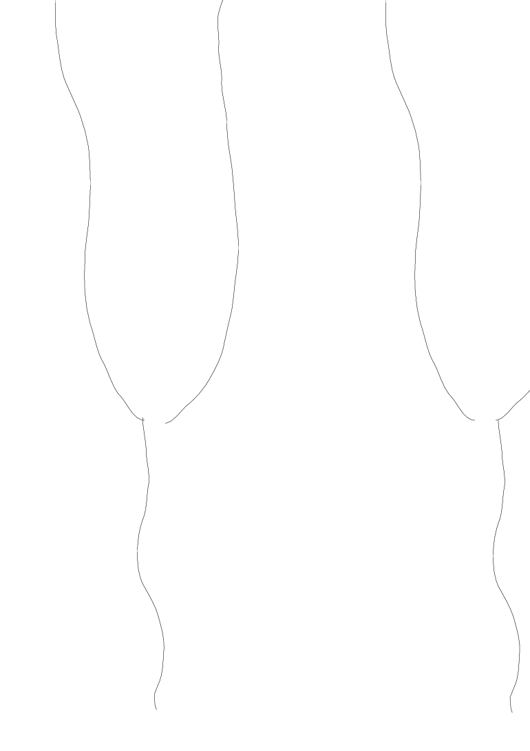
Refer to caption
Figure 2: In this pair of diagrams, tt is the vertical and xx the horizontal coordinate. If a (1,2)l(1,2)_{l} (left) point of the original web (left side of the figure) is marked to switch at some s0∈[0,s]s_{0}\in[0,s], then the direction of that (1,2)(1,2) point in the web 𝒲s\mathcal{W}^{s} is changed at s=s0s=s_{0} so that it becomes a (1,2)r(1,2)_{r} (right) point as on the right side of the figure with the incoming path joined to the rightmost of the two paths starting from that point.

At the discrete level the scaling is chosen in such a way that between the dynamical times 00 and ss, in a macroscopic box (i.e., one with size of order (δ)−1×δ−1(\sqrt{\delta})^{-1}\times\delta^{-1} in the original lattice), the number of arrows that change direction will be of order δ−1\delta^{-1}. The situation can be simplified by focusing on switchings with “macroscopic” effects (i.e., switchings that will lead to a macroscopic alteration of a walker’s trajectory in the initial web W0W^{0}). A priori, one should also consider combinations of switchings that have macroscopic effects, but it turns out (this will be proved rigorously in [NRS07]) that the probability of macroscopic effects from switching two or more arrows is negligible compared to switching single arrows, and can be neglected.

There is a natural way of characterizing those critical switchings. For example, let us consider the forward (rescaled) path SδS^{\delta} starting from the origin in W0W^{0} and assume that the arrow located at some (Sδ​(t),t)(S^{\delta}(t),t) is orginally oriented to the left. Now we ask whether a switching of this single arrow will alter the path in such a way that the altered path will be to the right of (Sδ​(t+Δ​t)+Δ​x,t+Δ​t)(S^{\delta}(t+\Delta t)+\Delta x,t+\Delta t), where (Δ​x,Δ​t)(\Delta x,\Delta t) are both positive macroscopic quantities. This will happen if and only if the backward path S^δ{\hat{S}}^{\delta} starting from (Sδ​(t+Δ​t)+Δ​x,t+Δ​t)(S^{\delta}(t+\Delta t)+\Delta x,t+\Delta t) hits SδS^{\delta} at time tt (more precisely, hits (Sδ​(t),t+δ)(S^{\delta}(t),t+\delta) at time t+δt+\delta). More generally, the critical arrows leading to similar alterations are the “contact” points between SδS^{\delta} and the backward path S^δ{\hat{S}}^{\delta} at which a switching occurs on [0,s][0,s]. But it is now fairly easy to see what the statistics of such a set of points are. In fact, let mδ​(t)m^{\delta}(t) be the random variable counting the number of such switchings up to the macroscopic time tt. The distribution of mδ​(t)m^{\delta}(t) is simply given by:

mδ​(t)\displaystyle m^{\delta}(t) =\displaystyle= ∑i=11δ​Lδ​(t)Xiδwith\displaystyle\sum_{i=1}^{\frac{1}{\sqrt{\delta}}L^{\delta}(t)}X_{i}^{\delta}\ \ \ \textrm{with}
Lδ​(t)\displaystyle L^{\delta}(t) =\displaystyle= δ#{k≤tδ:Sδ(kδ)=S^δ(kδ+δ)and there is a left arrow at (Sδ​(k​δ),k​δ)}\displaystyle\sqrt{\delta}\ \ \#\{k\leq\frac{t}{\delta}:S^{\delta}(k\delta)={\hat{S}}^{\delta}(k\delta+\delta)\ \ \ \textrm{and there is a left arrow at $(S^{\delta}(k\delta),k\delta)$}\}

where {Xiδ}\{X_{i}^{\delta}\} are i.i.d. Bernoulli random variables with ℙ⁡({Xiδ}=1)=1−exp⁡(−δ​λ​s)\mathbb{P}(\{X_{i}^{\delta}\}=1)=1-\exp{(-\sqrt{\delta}\lambda s}), which is δ​λ​s+o⁡(δ)\sqrt{\delta}\ \lambda s+o(\sqrt{\delta}) as δ→0\delta\to 0.

As δ→0\delta\to 0, LδL^{\delta} converges to the “local time” LL of the forward Brownian path B∈𝒲B\in\mathcal{W} starting from the origin along a backward Brownian path B^\hat{B} starting on the right of the path BB (the joint distribution of BB and B^\hat{B} is analysed in [STW00] and this “local time” will be defined precisely in [NRS07]). Further, it is a standard fact that t→∑i=1t/δXiδt\rightarrow\sum_{i=1}^{t/\sqrt{\delta}}X_{i}^{\delta} converges to a Poisson process. Hence, mδ​(t)m^{\delta}(t) will converge to a Poisson process run by the random clock λ​s​L​(t)\lambda\ sL(t). In other words, this set of points will consist of a two-dimensional (tt and ss) Poisson point process with intensity measure λ​d​L×l\lambda\ dL\times l, where ll is Lebesgue measure and d​LdL is the local time measure (note that λ​d​L×l\lambda\ dL\times l will be a locally finite measure so that the Poisson process is well defined).

So far, we have only selected the critical switchings inducing a specific type of macroscopic effect. Namely, the ones altering the path BB in such a way that a point originally on one side of BB will be on the opposite side after switching occurs. But in order to select all the critical arrows leading to any kind of macroscopic changes, we should not only consider a Poisson process run by the local time of a single forward path BB against a single backward path B^\hat{B}, but rather a Poisson process run by the “local time of the entire forward web along the entire backward web” multiplied by the intensity λ​s\lambda s. In other words, the set of marked points will be a three-dimensional Poisson point process with intensity measure λ​ℒ×l\lambda\ {\cal L}\times l, where ll is Lebesgue measure (in the variable ss) and ℒ{\cal L} is the local time measure of the forward web along the backward web. 11 1 Actually, the situation is a bit more complicated since ℒ{\cal L} would not be a locally finite measure — i.e., the set of marked points in space-time is actually dense in ℝ2\mathbb{R}^{2}. However, like what is presented in [FINR04] (see p. 11 there), one can add an extra coordinate and lift ℒ{\cal L} to be a σ\sigma-finite measure, or equivalently approximate ℒ{\cal L} by a sequence of locally finite measures ℒn{\cal L}_{n}, do the markings using ℒn{\cal L}_{n}, and then let n→∞n\to\infty.

Since the (1,2)(1,2) points of the continuum web are precisely those at which a forward and a backward path meet (see, e.g., [FINR04]), the measure λ​ℒ×l\lambda\ {\cal L}\times l will be supported by this set of points. From our previous description of them, it should be clear that each (1,2)(1,2) point has a preferred left or right “direction”. For example, a (1,2)r(1,2)_{r} (right) point is one for which the continuing path (coming in from earlier time) is to the right of the “newly-born” path. Hence, at the continuum level, the analog of an arrow switching will simply be a change of direction of all marked (1,2)(1,2) points (see Figure 2). The web 𝒲s\mathcal{W}^{s} at time s0s_{0} will be “simply” deduced from 𝒲0\mathcal{W}^{0} by switching the direction of all marked (1,2)(1,2) points whose ss-coordinate is in [0,s0][0,s_{0}].

A last comment concerns the nature of the dependence of the two continuum paths Bs​(t)B^{s}(t) and Bs′​(t)B^{s^{\prime}}(t). These turn out to be a pair of “sticky” Brownian motions, which are independent except when they touch each other. This is one of the major observations in [HW07]; we give a brief derivation of this fact in Section 2 by analyzing pairs of paths in the discrete setting to see what must occur in the continuum scaling limit. In Section 3, we state our main theorem about tameness; i.e., that there are no exceptional dynamical times when the random walkers are transient. We also give there some other results about tameness in two extended remarks — one about non-coalescence and the other about two-sided bounds of order t\sqrt{t}. Then in Section 4, we show that there are exceptional dynamical times when the walkers are (weakly) subdiffusive — i.e., have one-sided bounds of order t\sqrt{t}. In Section 5 we derive upper and lower bounds on the Hausdorff dimension of the set of such exceptional dynamical times. Some estimates for random walks that are needed for our arguments are given in Appendix A.

2 Pairs Of Paths In The Dynamical Discrete Web

2.1 Interaction Between Paths In WsW^{s} And Ws′W^{s^{\prime}}

The dynamics can be described, equivalently to the definition in Section 1, in the following manner. The initial configuration is set to ξ0\xi_{0}, but now we place independent Poisson clocks at each site (i,j)(i,j) that ring at rate λ\lambda. Every time clocks ring we toss independent fair coins to decide on the values of ξi,j\xi_{i,j} after the ring. Statistically the two descriptions are equivalent.

The motivation for this second description is that it leads to a useful representation of the interaction between the discrete webs at different dynamical times ss and s′>ss^{\prime}>s. In particular, let SsS^{s} and Ss′S^{s^{\prime}} be the walks starting at (0,0)(0,0) and defined for times t=0,1,2,…t=0,1,2,\dots, belonging to WsW^{s} and Ws′W^{s^{\prime}}.

If Ss​(t)≠Ss′​(t)S^{s}(t)\neq S^{s^{\prime}}(t), then Ss​(t+1)−Ss​(t)S^{s}(t+1)-S^{s}(t) and Ss′​(t+1)−Ss′​(t)S^{s^{\prime}}(t+1)-S^{s^{\prime}}(t) are independent since the directions of the arrows at two distinct sites are independent. On the other hand, if Ss​(t)=Ss′​(t)S^{s}(t)=S^{s^{\prime}}(t), then the next steps of the two walks are now correlated. If the clock at the site (Ss​(t),t)(S^{s}(t),t) did not ring on [s,s′)[s,s^{\prime}), then the two paths will coincide at time t+1t+1. If it rang at least once, then with probability 12\frac{1}{2} they will coincide, and with probabily 12\frac{1}{2} they won’t.

Let us now define inductively a sequence of pairs of stopping times (τi,σi)(\tau_{i},\sigma_{i}) with τ0=σ0=0\tau_{0}=\sigma_{0}=0 and:

τi+1=inf{t>σi:Ss​(t)=Ss′​(t)}\displaystyle\tau_{i+1}=\inf\{t>\sigma_{i}:\ S^{s}(t)=S^{s^{\prime}}(t)\} (1)
σi=inf{t≥τi:the clock at(Ss(t),t)rings in[s,s′)}\displaystyle\sigma_{i}=\inf\{t\geq\tau_{i}:\ \ \textrm{the clock at}\ (S^{s}(t),t)\ \textrm{rings in}\ [s,s^{\prime})\} (2)

On the interval of integer time [τi,σi][\tau_{i},\sigma_{i}], the paths Ss,Ss′S^{s},S^{s^{\prime}} coincide and at time σi\sigma_{i} they decide to separate with probability 12\frac{1}{2}. In other words, from time σi\sigma_{i}, the walkers (Ss,Ss′)(S^{s},S^{s^{\prime}}) move independently until the next meeting time τi+1\tau_{i+1}. Hence, if we skip the intervals of time {[τi,σi)}i\{[\tau_{i},\sigma_{i})\}_{i}, (Ss,Ss′)(S^{s},S^{s^{\prime}}) behave as two independent random walks (S1,S2)(S_{1},S_{2}), while if we skip the intervals {[σi,τi+1)}i\{[\sigma_{i},\tau_{i+1})\}_{i}, the two walks coincide with a single random walk S3S_{3}. Furthermore, since S3S_{3} is constucted from the arrow configuration at different sites than the ones used to construct (S1,S2)(S_{1},S_{2}), it is independent of (S1,S2)(S_{1},S_{2}) ; and {σi−τi}\{\sigma_{i}-\tau_{i}\} are i.i.d. random variables with ℙ⁡(σi−τi≥k)=(e−λ​|s−s′|)k\mathbb{P}(\sigma_{i}-\tau_{i}\geq k)=(e^{-\lambda|s-s^{\prime}|})^{k}.

Now, skipping the intervals {[τi,σi)}i\{[\tau_{i},\sigma_{i})\}_{i} corresponds to making the random time change t→C⁡(t)t\rightarrow C(t) with (C)−1​(t)=L^​(t)+t(C)^{-1}(t)={\hat{L}}(t)+t, and

  1. 1.

    L^​(t)=∑i=1l^​(t)σi−τi{\hat{L}}(t)=\sum_{i=1}^{{\hat{l}}(t)}\sigma_{i}-\tau_{i}   ,

  2. 2.

    l^​(t)=#⁡{k≤t:S1​(k)=S2​(k)}{\hat{l}}(t)=\#\{k\leq t:S_{1}(k)=S_{2}(k)\}   ,

while skipping {[σi,τi+1)}i\{[\sigma_{i},\tau_{i+1})\}_{i} corresponds to making the time change t→t−C⁡(t)t\rightarrow t-C(t); i.e.,

Ss​(t)=S1​(C⁡(t))+S3​(t−C⁡(t)),\displaystyle S^{s}(t)=S_{1}(C(t))+S_{3}(t-C(t)), (3)
Ss′​(t)=S2​(C⁡(t))+S3​(t−C⁡(t)),\displaystyle S^{s^{\prime}}(t)=S_{2}(C(t))+S_{3}(t-C(t)), (4)

where (S1,S2,S3)(S_{1},S_{2},S_{3}) are three independent standard random walks. In the following (S~1,S~2)(\tilde{S}_{1},\tilde{S}_{2}), distributed as (Ss,Ss′)(S^{s},S^{s^{\prime}}), will be referred to as a pair of sticky random walks.

Refer to caption
Figure 3: For tt fixed, this graph represents s→Ss​(t)s\rightarrow S^{s}(t) starting from x=60x=60 (with t=200t=200 and λ=1200\lambda=\frac{1}{\sqrt{200}}).

2.2 Sticky Paths In The Scaling Limit

Time and space are respectively rescaled by δ−1\delta^{-1} and δ−1/2\delta^{-1/2} and the rate of switching is taken as λ=λ¯​δ\lambda={\bar{\lambda}}\sqrt{\delta}. From the previous section, the pair of rescaled processes (δ​Ss​(tδ),δ​Ss′​(tδ))(\sqrt{\delta}S^{s}(\frac{t}{\delta}),\sqrt{\delta}S^{s^{\prime}}(\frac{t}{\delta})) is statistically equivalent to

S~1δ=S1δ​(Cδ​(t))+S3δ​(t−Cδ​(t))\tilde{S}_{1}^{\delta}=S_{1}^{\delta}(C^{\delta}(t))+S_{3}^{\delta}(t-C^{\delta}(t)) (5)
S~2δ=S2δ​(Cδ​(t))+S3δ​(t−Cδ​(t))\tilde{S}_{2}^{\delta}=S_{2}^{\delta}(C^{\delta}(t))+S_{3}^{\delta}(t-C^{\delta}(t)) (6)

where S1δ,S2δ,S3δS_{1}^{\delta},S_{2}^{\delta},S_{3}^{\delta} are three independent rescaled random walks, and (Cδ)−1​(t)=L^δ​(t)+t(C^{\delta})^{-1}(t)={\hat{L}}^{\delta}(t)+t with

  1. 1.

    L^δ(t)=δ∑i=1l^δ(t)δ−1/2Ti{\hat{L}}^{\delta}(t)={\delta}\sum_{i=1}^{{\hat{l}}^{\delta}(t){\delta}^{-1/2}}T_{i}

  2. 2.

    l^δ​(t)=δ​#​{k≤t/δ:S1δ​(k​δ)=S2δ​(k​δ)}{\hat{l}}^{\delta}(t)=\sqrt{\delta}\#\{k\leq t/{\delta}:S_{1}^{\delta}(k\delta)=S_{2}^{\delta}(k\delta)\}

  3. 3.

    {Ti}\{T_{i}\} are i.i.d random variables taking values in ℕ\mathbb{N}, with ℙ⁡(Ti≥k)=e−k​λ​|s−s′|\mathbb{P}(T_{i}\geq k)=e^{-k\ \lambda|s-s^{\prime}|}.

As δ→0\delta\to 0, (S1δ,S2δ,S3δ)(S_{1}^{\delta},S_{2}^{\delta},S_{3}^{\delta}) converges in distribution to three independent Brownian motions (B1,B2,B3)(B_{1},B_{2},B_{3}); and l^δ{\hat{l}}^{\delta} converges in distribution to the local time L~{\tilde{L}} at the origin of |B1−B2||B_{1}-B_{2}|. Moreover, as a consequence of the Law of Large Numbers, if we take λ=λ¯​δ\lambda=\bar{\lambda}\sqrt{\delta}, with λ¯\bar{\lambda} of order 11, then L^δ​(t){\hat{L}}^{\delta}(t) converges to (|s−s′|​λ¯)−1​L~​(t)({|s-s^{\prime}|\bar{\lambda}})^{-1}{\tilde{L}}(t). Hence, it should come as no surprise that (S~1δ,S~2δ)(\tilde{S}_{1}^{\delta},\tilde{S}_{2}^{\delta}) converges to

B~1=B1​(C⁡(t))+B3​(t−C⁡(t))\displaystyle\tilde{B}_{1}=B_{1}(C(t))+B_{3}(t-C(t)) (7)
B~2=B2​(C⁡(t))+B3​(t−C⁡(t))\displaystyle\tilde{B}_{2}=B_{2}(C(t))+B_{3}(t-C(t)) (8)

where now C−1​(t)=t+(|s−s′|​λ¯)−1​L~​(t)C^{-1}(t)=t+({|s-s^{\prime}|\bar{\lambda}})^{-1}{\tilde{L}}(t), which is identical in distribution to a pair of sticky Brownian motions with stickiness parameter (|s−s′|​λ¯)−1({|s-s^{\prime}|\bar{\lambda}})^{-1} (see, e.g., [SS06]).

We note that for small δ\delta, the location S~δ,s​(t){\tilde{S}}^{\delta,s}(t), of the path starting from some (x0,t0)(x_{0},t_{0}) is, for fixed tt, quite discontinuous in ss — see Figure 3.

3 Tameness

Theorem 1.

Almost surely, all the paths are recurrent for every ss.

Proof.

In Section 3 of [HPS97], it is proved that for any homogeneous graph with critical probability pcp_{c} for percolation and such that θ⁡(p)\theta(p), the probability that (with parameter pp) the origin belongs to an infinite cluster, satisfies θ⁡(p)≤C⁡(p−pc)\theta(p)\leq C(p-p_{c}) for p≥pcp\geq p_{c}, there is almost surely no dynamical time ss at which percolation occurs.

In our setting, an entirely parallel argument can be used to show tameness of the dynamical discrete web with respect to recurrence. We discuss this briefly below, pointing to the relevant parts of [HPS97].

We consider the event Ai,jA_{i,j} that the walker starting from (i,j)(i,j) does not visit the site to the left of its starting position, that is, that the path S(i,j)S_{(i,j)} started at (i,j)(i,j) does not contain any (i−1,k)(i-1,k) with k>jk>j. Let θ~​(p)\tilde{\theta}(p) be the probability of that event under pp — i.e., when the random walk increments are +1+1 (resp., −1-1) with probability pp (resp., 1−p1-p). Under the usual coupled construction of the model for p∈[0,1]p\in[0,1], this event is increasing with pp in [1/2,1][1/2,1]. For p>12p>\frac{1}{2} (resp. p<12p<\frac{1}{2}), S(i,j)S_{(i,j)} is distributed as a right (resp. left) drifting random walk. In particular, it is well known that for p∈[1/2,1]p\in[1/2,1]

θ~​(p)=(2​p−1)/p.\tilde{\theta}(p)=(2p-1)/p. (9)

We now describe the parallel argument alluded to above. Let N~i,j\tilde{N}_{i,j} denote the cardinality of the set {s∈[0,1]:Ai,j​ occurs in ​(ξ)s}\{s\in[0,1]:\,A_{i,j}\mbox{ occurs in }(\xi)_{s}\}. θ~​(p)\tilde{\theta}(p) and N~i,j\tilde{N}_{i,j} are the analogues of θv​(p)\theta_{v}(p) and NvN_{v} in Section 3 of [HPS97]. An analogue of Lemma 3.1 there also holds here with the same proof, where here 1/21/2 is the analogue of pcp_{c} there, and the analogue of Nv,mN_{v,m} is the number N~i,j,m\tilde{N}_{i,j,m} of k∈{1,2,…,m}k\in\{1,2,\ldots,m\} such that Ai,jA_{i,j} occurs in

ξ¯(k)={ξ¯i′,j′(k)=maxs∈[(k−1)/m,k/m]⁡ξi′,j′s,(i′,j′)∈ℤe​v​e​n},\bar{\xi}^{(k)}=\left\{\bar{\xi}^{(k)}_{i^{\prime},j^{\prime}}=\max_{s\in[(k-1)/m,k/m]}\xi^{s}_{i^{\prime},j^{\prime}},\,(i^{\prime},j^{\prime})\in{\mathbb{Z}}_{even}\right\},

and we conclude from (9) that 𝔼⁡(N~i,j)<∞{\mathbb{E}}(\tilde{N}_{i,j})<\infty. Analogues of Lemmas 3.2 and 3.4 also hold with the same proofs for the analogue quantities, and with Ai,jA_{i,j} replacing the event {v percolates}. We then have that 𝔼⁡(N~i,j)=0{\mathbb{E}}(\tilde{N}_{i,j})=0, and thus almost surely for every ss every walker eventually visits the site to the left of its starting position. The same is of course true of the site to the right of the starting position by symmetry. We conclude that almost surely for every tt every walker eventually visits every site in ℤ{\mathbb{Z}} (infinitely often). ∎

Remark 1.

Another property of the static discrete web with respect to which the dynamical one is tame is the almost sure coalescence of all of its paths. It is enough to consider the case of two paths. For those, a similar argument as that for recurrence holds. The analogue objects to be considered in this case are as follows. Given v,v′∈ℤe​v​e​nv,v^{\prime}\in{\mathbb{Z}}_{even} (let us assume that v1<v1′,v2=v2′v_{1}<v^{\prime}_{1},v_{2}=v^{\prime}_{2}), let Cv,v′C_{v,v^{\prime}} be the event that the paths starting from v,v′v,v^{\prime} do not eventually coalesce, and let N~v,v′\tilde{N}_{v,v^{\prime}} be the cardinality of the set {s∈[0,1]:Cv,v′​ occurs in ​(ξ)s}\{s\in[0,1]:\,C_{v,v^{\prime}}\mbox{ occurs in }(\xi)_{s}\}. For 1≤k≤m1\leq k\leq m, let also Cv,v′,k,mC_{v,v^{\prime},k,m} be the event that the path of ξ¯(k)\bar{\xi}^{(k)} starting from v′v^{\prime} and that of ξ¯(k)\underline{\xi}^{(k)} starting from vv do not coalesce eventually, where

ξ¯(k)={ξ¯i,j(k)=mins∈[(k−1)/m,k/m]⁡ξi,js,(i,j)∈ℤe​v​e​n}.\underline{\xi}^{(k)}=\left\{\underline{\xi}^{(k)}_{i,j}=\min_{s\in[(k-1)/m,k/m]}\xi^{s}_{i,j},\,(i,j)\in{\mathbb{Z}}_{even}\right\}.

Let now N~v,v′,m\tilde{N}_{v,v^{\prime},m} be the number of k∈{1,2,…,m}k\in\{1,2,\ldots,m\} such that Cv,v′,k,mC_{v,v^{\prime},k,m} occurs. To show that 𝔼⁡(N~v,v′)=0{\mathbb{E}}(\tilde{N}_{v,v^{\prime}})=0, we analyze N~v,v′,m\tilde{N}_{v,v^{\prime},m} and its related quantities analogously to the analysis of N~i,j,m\tilde{N}_{i,j,m} and its related quantities to show that 𝔼⁡(N~i,j)=0{\mathbb{E}}(\tilde{N}_{i,j})=0. In particular, the fact that ℙ⁡(Cv,v′,k,m)≤const./m{\mathbb{P}}(C_{v,v^{\prime},k,m})\leq\mbox{const.}/m follows from standard random walk estimates, using the fact that the difference of two random walk paths is another random walk path.

Remark 2.

A main result of this paper is the existence of exceptional ss such that for all tt, Ss​(t)≥−k−K​tS^{s}(t)\geq-k-K\sqrt{t} (see Theorem 2 in Section 4), and of course there are then also exceptional ss such that Ss​(t)≤k+K​tS^{s}(t)\leq k+K\sqrt{t}. However, it can be shown that there are no exceptional ss for the two-sided bound |Ss​(t)|≤k+K​t|S^{s}(t)|\leq k+K\sqrt{t}, at least for small enough KK. The precise condition on KK under which we can prove this result is that 1−2​p​(K)≤1/21-2p(K)\leq 1/2, where p⁡(K)p(K) is defined in Proposition 3 below. Note that this condition implies according to Proposition 3 that the Hausdorff dimension of the set of exceptional ss for either of the corresponding one-sided bounds does not exceed 1/21/2. The proof of this tameness claim combines arguments like those of Theorem 1 and Remark 1 with the estimates of Lemma 5 and Proposition 4 and with an application of the FKG inequalities. The specific FKG inequality, for the two events Uϵ±U_{\epsilon}^{\pm} that for some s∈[0,ϵ]s\in[0,\epsilon] and all tt, ±Ss​(t)≥−k−K​t\pm S^{s}(t)\geq-k-K\sqrt{t}, is that ℙ⁡(Uϵ+∩Uϵ−)≤ℙ⁡(Uϵ+)⋅ℙ⁡(Uϵ−)\mathbb{P}(U_{\epsilon}^{+}\cap U_{\epsilon}^{-})\leq\mathbb{P}(U_{\epsilon}^{+})\,\cdot\,\mathbb{P}(U_{\epsilon}^{-}). This is so because Uϵ+U_{\epsilon}^{+} (resp., Uϵ−U_{\epsilon}^{-}) is an increasing (resp., decreasing) event with respect to the basic ξ(i,j)s\xi_{(i,j)}^{s} processes — see, e.g., Lemma 3.3 of [HPS97] for more details. We finally note that by essentially the same arguments one obtains tameness for two-sided bounds of the form −k1−K1​t≤Ss​(t)≤k2+K2​t-k_{1}-K_{1}\sqrt{t}\leq S^{s}(t)\leq k_{2}+K_{2}\sqrt{t} provided that K1,K2K_{1},K_{2} are small enough that (1−2​p​(K1))+(1−2​p​(K2))≤1(1-2p(K_{1}))+(1-2p(K_{2}))\leq 1.

4 Existence of Exceptional Times

Let {d⁡(k)}k≥0\{d(k)\}_{k\geq 0} be a sequence of positive integers divisible by 44. We construct inductively a sequence of “diffusive” boxes BkB_{k} in the following manner:

  • •

    B0B_{0} is the rectangle with vertices (−12​d​(0),0)(-\frac{1}{2}\ d(0),0), (+12​d​(0),0)(+\frac{1}{2}\ d(0),0), (−12​d​(0),d​(0)2)(-\frac{1}{2}\ d(0),d(0)^{2}) and (+12​d​(0),d​(0)2)(+\frac{1}{2}d(0),d(0)^{2}).

  • •

    Let zn=(xn,tn)z_{n}=(x_{n},t_{n}) and zn′′z_{n}^{{}^{\prime\prime}} be respectively the middle point of the lower edge and the upper right vertex of BnB_{n}. Bn+1B_{n+1} is the rectangle of height d​(n+1)2d(n+1)^{2} and width d⁡(n+1)d(n+1) such that zn+1z_{n+1} equals zn′′z_{n}^{{}^{\prime\prime}} (see Figure 4).

Let AksA_{k}^{s} be the event that the path of WsW^{s} starting at zkz_{k} is at or to the right of zk′′z_{k}^{{}^{\prime\prime}} at time tk+1t_{k+1} and that it is never to the left of the left edge ∂k\partial_{k} of the box BkB_{k} . We would like to prove that for a certain choice of {d⁡(k)}\{d(k)\}, there exist some exceptional times ss at which {Aks}\{A_{k}^{s}\} occurs for every kk. At those times, this would imply that the path starting from the origin stays to the right of the graphs obtained by patching together the left edges, ∂k\partial_{k}, (see Figure 4). By the same kind of reasoning used in dynamical percolation [SS05], to prove that ordinary diffusive behavior does not occur at certain exceptional dynamical times ss, it suffices to derive the following lemma, which we do later in this section of the paper.

Refer to caption
Figure 4: Construction of the first three boxes (B0,B1,B2)(B_{0},B_{1},B_{2}) with tt the vertical and xx the horizontal coordinate. The solid curves represent segments of the paths starting from z0z_{0}, z1=z0′′z_{1}=z_{0}^{{}^{\prime\prime}} and z2=z1′′z_{2}=z_{1}^{{}^{\prime\prime}} for which the events A0sA_{0}^{s}, A1sA_{1}^{s} and A2sA_{2}^{s} occur. The leftmost curve represents −k−K​t-k-K\sqrt{t}.
Lemma 1.

There exists γ0>2\gamma_{0}>2 such that if d​(k)=4​([γk4​λ]+1)d(k)=4([\frac{\gamma^{k}}{4\lambda}]+1) for k≥0k\geq 0 (where [x][x] is the integer part of xx) with γ>γ0\gamma>\gamma_{0}, then

infnℙ⁡(∫01∏k=0n1Aks​𝑑s> 0)≥p,\inf_{n}\mathbb{P}(\int_{0}^{1}\prod_{k=0}^{n}1_{A_{k}^{s}}\ ds>\ 0)\geq p, (10)

where pp is bounded away from 00 when λ\lambda is bounded away from ∞\infty.

Let EnE_{n} be the set of times ss on [0,1][0,1] such that ⋂k=0nAks\bigcap_{k=0}^{n}A_{k}^{s} occurs. The previous lemma implies that ℙ⁡(⋂n=0∞(En≠∅))≥p>0\mathbb{P}(\bigcap_{n=0}^{\infty}(E_{n}\neq\emptyset))\geq p>0. Since {En}\{E_{n}\} is obviously decreasing in nn, if the EnE_{n} were closed subsets of [0,1][0,1] it would follow that ℙ⁡(⋂n=0∞En≠∅)≥p>0\mathbb{P}(\bigcap_{n=0}^{\infty}E_{n}\ \neq\emptyset)\geq p>0. As explained in the proof of the next theorem, for s∈⋂n=0∞Ens\in\bigcap_{n=0}^{\infty}E_{n}, Ss​(t)≥−k−K​tS^{s}(t)\geq-k-K\sqrt{t} for some k,K<∞k,K<\infty (depending on γ\gamma) and all t=0,1,2,…t=0,1,2,\dots. Unfortunately, the set of times at which one arrow is (or any finitely many are) oriented to the right (resp., to the left) is not a closed subset of [0,1][0,1] since we have a right continuous process, and thus EnE_{n} is not a closed set. This extra technicality is handled like in Lemma 5.1 in [SS05], as follows. Let 𝒮^\hat{\cal S} denote the (random) set of all switching times for all ξi,js\xi_{i,j}^{s}’s. By modifying every ξi,js\xi_{i,j}^{s} so that for s′∈𝒮^s^{\prime}\in\hat{\cal S}, ξi,js′=+1\xi_{i,j}^{s^{\prime}}=+1 (rather than being right-continuous), each EnE_{n} is replaced by a closed E¯n⊇En{\bar{E}}_{n}\supseteq E_{n}. On the other hand, ∩n=1∞E¯n=∩n=1∞En\cap_{n=1}^{\infty}{\bar{E}}_{n}=\cap_{n=1}^{\infty}E_{n} as a consequence of the fact that 𝒮^\hat{\cal S} is countable and by independence of the ξi,j\xi_{i,j}’s no s′∈𝒮^s^{\prime}\in\hat{\cal S} can be exceptional.

The uniformity with respect to small λ\lambda in Lemma 1 means that once space and time are diffusively rescaled by δ−12\delta^{-\frac{1}{2}} and δ−1\delta^{-1} and λ\lambda is rescaled by δ12\delta^{\frac{1}{2}}, the inequality (10) is still valid, with pp fixed as δ→0\delta\to 0.

As a consequence of Lemma 1, we will obtain the following.

Theorem 2.

(violation of the CLT) For λ¯,δ∈(0,∞){\bar{\lambda}},\delta\in(0,\infty), let Sδs​(t)=Sδ,λ¯s​(t)=δ​Ss​([t/δ])S^{s}_{\delta}(t)=S_{\delta,\bar{\lambda}}^{s}(t)=\sqrt{\delta}S^{s}([t/\delta]) where Ss​(⋅)=S1,λs​(⋅)S^{s}(\cdot)=S^{s}_{1,\lambda}(\cdot) is the path starting at (0,0)(0,0) of the dynamical discrete web with switching rate λ=λ¯​δ\lambda=\bar{\lambda}\sqrt{\delta}. There exists K<∞K<\infty such that pδ,λ¯​(K,k¯)p_{\delta,\bar{\lambda}}(K,\bar{k}), the probability to have a nonempty set of exceptional times s in [0,1][0,1] for which Sδ,λ¯s​(t)≥−k¯−K​tS^{s}_{\delta,\bar{\lambda}}(t)\geq-\bar{k}-K\sqrt{t} for all t≥0t\geq 0 satisfies the following:

  1. 1.

    For any k¯>0\bar{k}>0, there exist λ¯0,λ0∈(0,∞)\bar{\lambda}_{0},\lambda_{0}\in(0,\infty) such that

    infλ¯≥λ¯0,δ≤(λ0/λ¯0)2pδ,λ¯​(K,k¯)>0.\inf_{\bar{\lambda}\geq\bar{\lambda}_{0},\ \delta\leq({\lambda_{0}}/{\bar{\lambda}_{0}})^{2}}p_{\delta,\bar{\lambda}}(K,\bar{k})>0\,. (11)
  2. 2.

    Similarly, for any λ¯0\bar{\lambda}_{0}, λ0∈(0,∞)\lambda_{0}\in(0,\infty), there exists k¯<∞\bar{k}<\infty such that (11) is valid.

  3. 3.

    For any fixed δ\delta, λ¯∈(0,∞)\bar{\lambda}\in(0,\infty), pδ,λ¯​(K,0)>0p_{\delta,\bar{\lambda}}(K,0)>0.

Proof.

In the unrescaled coordinates, we take boxes BkB_{k} as in Lemma 1 with d(k)=4([γk4​λ]+1)∈(γk/λ,4+γk/λ]d(k)=4([\frac{\gamma^{k}}{4\lambda}]+1)\in(\gamma^{k}/\lambda,4+\gamma^{k}/\lambda]. Then in rescaled coordinates we have boxes B¯k{\bar{B}}_{k} with (spatial) width d¯(k)=(λ/λ¯)d(k)∈(γk/λ¯,4δ+γk/λ¯]{\bar{d}}(k)=(\lambda/\bar{\lambda})d(k)\in(\gamma^{k}/\bar{\lambda},4\sqrt{\delta}+\gamma^{k}/\bar{\lambda}] and (temporal) height d¯​(k)2{\bar{d}}(k)^{2}. Let ∂¯{\bar{\partial}} denote the right-continuous function obtained by joining together the left boundaries ∂¯k{\bar{\partial}}_{k} of B¯k{\bar{B}}_{k}. On [t¯n,t¯n+1)[{\bar{t}}_{n},{\bar{t}}_{n+1}) with t¯n=d¯​(0)2+d¯​(1)2+…​d¯​(n−1)2{\bar{t}}_{n}=\bar{d}(0)^{2}+\bar{d}(1)^{2}+\dots\bar{d}({n-1})^{2}, we have ∂¯​(t)=∂¯​(t¯n)=x¯n−(1/2)​d¯​(n){\bar{\partial}}(t)={\bar{\partial}}({\bar{t}}_{n})={\bar{x}}_{n}-(1/2){\bar{d}}(n) =(d¯​(0)+d¯​(1)+⋯+d¯​(n−1)−d¯​(n))/2=(\bar{d}(0)+\bar{d}(1)+\dots+\bar{d}(n-1)-\bar{d}(n))/2. If K,k¯K,\bar{k} are such that

∂¯​(t¯n)≥−(k¯+K​t¯n)​for​n=0,1,2,…,{\bar{\partial}}({\bar{t}}_{n})\ \geq\ -(\bar{k}+K\sqrt{{\bar{t}}_{n}})\ \textrm{for}\ n=0,1,2,\dots\ , (12)

then we will have ∂¯​(t)≥−(k¯+K​t){\bar{\partial}}(t)\geq-(\bar{k}+K\sqrt{t}) for all t≥0t\geq 0 as desired.

The inequality (12) can be rewritten as

d¯​(n)≤2​k¯+d¯​(0)+⋯+d¯​(n−1)+2​K​[d¯​(0)2+⋯+d¯​(n−1)2]1/2.\bar{d}(n)\leq 2\bar{k}+\bar{d}(0)+\cdots+\bar{d}(n-1)+2K[{\bar{d}(0)}^{2}+\cdots+{\bar{d}(n-1)}^{2}]^{1/2}\,. (13)

Using the bound d¯​(n)≤4​δ+γn/λ¯\bar{d}(n)\leq 4\sqrt{\delta}+\gamma^{n}/\bar{\lambda} on the left-hand side of (13) and the bounds d¯​(j)≥γj/λ¯\bar{d}(j)\geq\gamma^{j}/\bar{\lambda} on the right-hand side, it follows that in order to verify (13) it suffices to have, for n=0,1,2,…n=0,1,2,\dots,

γn≤(2​k¯−4​δ)​λ¯+γn−1γ−1+2​K​γ2​n−1γ2−1.\gamma^{n}\leq(2\bar{k}-4\sqrt{\delta})\bar{\lambda}+\frac{\gamma^{n}-1}{\gamma-1}+2K\sqrt{\frac{\gamma^{2n}-1}{\gamma^{2}-1}}\ . (14)

Using the elementary bound γ2​n−1≥γn​(1−γ−2​n)\sqrt{\gamma^{2n}-1}\geq\gamma^{n}(1-\gamma^{-2n}) (for γ≥1\gamma\geq 1), we see that in order to verify (14), it suffices to have, for n=0,1,2,…n=0,1,2,\dots,

γn​(γ−2γ−1−2​Kγ2−1)≤(2​k¯−4​δ)​λ¯−1γ−1−2​Kγ2−1​γ−n.\gamma^{n}(\frac{\gamma-2}{\gamma-1}-\frac{2K}{\sqrt{\gamma^{2}-1}})\leq(2\bar{k}-4\sqrt{\delta})\bar{\lambda}-\frac{1}{\gamma-1}-\frac{2K}{\sqrt{\gamma^{2}-1}}\gamma^{-n}\,. (15)

Choosing K=(γ−22)​γ+1γ−1K=(\frac{\gamma-2}{2})\sqrt{\frac{\gamma+1}{\gamma-1}} yields this inequality provided (2​k¯−4​δ)​λ¯−1≥0(2\bar{k}-4\sqrt{\delta})\bar{\lambda}-1\geq 0. It is easy to see that for any k¯>0\bar{k}>0, this will be valid provided λ0\lambda_{0} is small enough and λ¯0\bar{\lambda}_{0} is large enough so that k¯≥2​λ0/λ¯0+1/(2​λ¯0)\bar{k}\geq 2\lambda_{0}/\bar{\lambda}_{0}+1/(2\bar{\lambda}_{0}). This and Lemma 1 prove the first claim of the theorem; the second claim, in which λ¯0\bar{\lambda}_{0} and λ0\lambda_{0} are given, follows similarly.

We now turn to the proof of the final claim. We set δ=1\delta=1 since essentially the same proof works for any δ>0\delta>0. Let Tm[0,1]T_{m}^{[0,1]} denote the set of s∈[0,1]s\in[0,1] such that Ss​(n)≥−m−K​nS^{s}(n)\geq-m-K\sqrt{n} for n≥0n\geq 0 and let jj be an integer so large that (by the second claim of the theorem) p1,λ¯​(K,j)>0p_{1,\bar{\lambda}}(K,j)>0. First, T0[0,1]⊃T^j[0,1]⋂{s∈[0,1]:ξm,ms=+1form<j}T_{0}^{[0,1]}\supset\hat{T}_{j}^{[0,1]}\bigcap\{s\in[0,1]:\xi_{m,m}^{s}=+1\ \ \textrm{for}\ \ m<j\} where T^j[0,1]\hat{T}_{j}^{[0,1]} is the set of s∈[0,1]s\in[0,1] such that S(j,j)s​(n)≥−K​nS^{s}_{(j,j)}(n)\geq-K\sqrt{n} for n≥jn\geq j. Furthermore, T^j[0,1]⊃T¯j[0,1]\hat{T}_{j}^{[0,1]}\supset\bar{T}_{j}^{[0,1]}, where T¯j[0,1]\bar{T}_{j}^{[0,1]} is the set of s∈[0,1]s\in[0,1] such that S(j,j)s​(n)−j≥−j−K​n−jS^{s}_{(j,j)}(n)-j\geq-j-K\sqrt{n-j} for n≥jn\geq j. But T¯j[0,1]\bar{T}_{j}^{[0,1]} is just the translation (from (0,0)(0,0) to (j,j)(j,j)) of Tj[0,1]T_{j}^{[0,1]}. Since {s∈[0,1]:∀k<j,ξk,ks=+1}\{s\in[0,1]:\forall\ k<j,\ \xi_{k,k}^{s}=+1\} and T¯j[0,1]\bar{T}_{j}^{[0,1]} are independent, it follows that

p1,λ¯(K,0)≥p1,λ¯(K,j)ℙ(∀s∈[0,1],∀k<n,ξk,ks=+1)>0.p_{1,\bar{\lambda}}(K,0)\ \geq\ p_{1,\bar{\lambda}}(K,j)\ \ \mathbb{P}(\forall\ s\in[0,1],\ \forall\ k<n,\ \ \xi_{k,k}^{s}=+1)>0\,. (16)

∎

In particular, if we assume that s→Wδss\rightarrow W_{\delta}^{s} converges to the dynamical Brownian web (see Subsection 1.5) in some appropriate sense as δ→0\delta\to 0, this shows that the analogue of Theorem 3 (except for the final claim with δ\delta fixed and k¯=0\bar{k}=0) will be valid for the continuum model as well.

We now turn to:

Proof of Lemma 1. By the Cauchy-Schwarz inequality,

ℙ⁡(∫01∏k=0n1Aks​𝑑s>0)\displaystyle\mathbb{P}(\int_{0}^{1}\prod_{k=0}^{n}1_{A_{k}^{s}}\ ds>0) ≥\displaystyle\geq (𝔼⁡[∫01∏k=0n1Aks​𝑑s])2𝔼⁡[(∫01∏k=0n1Aks​𝑑s)2]\displaystyle\frac{\left(\mathbb{E}\left[\int_{0}^{1}\prod_{k=0}^{n}1_{A_{k}^{s}}\ ds\right]\right)^{2}}{\mathbb{E}\left[\left(\int_{0}^{1}\prod_{k=0}^{n}1_{A_{k}^{s}}\ ds\right)^{2}\right]} (17)
=\displaystyle= ([∫01∫01∏k=0nℙ⁡(Aks​⋂Aks′)ℙ​(Ak)2​𝑑s​d​s′])−1\displaystyle\left(\left[\int_{0}^{1}\int_{0}^{1}\prod_{k=0}^{n}\frac{\mathbb{P}(A_{k}^{s}\bigcap A_{k}^{s^{\prime}})}{\mathbb{P}(A_{k})^{2}}\ ds\ ds^{\prime}\right]\right)^{-1} (18)

where Ak=Ak0A_{k}=A_{k}^{0} and the equality is a consequence of the stationarity of s→Wss\rightarrow W^{s} and the independence between the different boxes BkB_{k}. It is enough to show that the integrand in the last expression of (18) is bounded above by a integrable function on [0,1]×[0,1][0,1]\times[0,1], uniformly in nn. The rest of the proof will verify this property.

Now, for fixed kk and two deterministic times (s,s′)(s,s^{\prime}), let us rescale space and time respectively by δ−1/2=d(k)\delta^{-1/2}={d(k)} and δ−1=d​(k)2\delta^{-1}=d(k)^{2}. Also, let S~1δ,S~2δ\tilde{S}_{1}^{\delta},\tilde{S}_{2}^{\delta} be the paths starting at 1/21/2 at time 00, defined as the rescaled and translated version of the paths (S1,S2)∈(Ws,Ws′)(S_{1},S_{2})\in(W^{s},W^{s^{\prime}}) starting at zkz_{k}, the middle point of the lower segment of the box BkB_{k}. (S~1δ,S~2δ)(\tilde{S}_{1}^{\delta},\tilde{S}_{2}^{\delta}) is a pair of sticky rescaled random walks starting at 1/21/2 at time t=0t=0 whose statistics (up to a translation of starting point) are described in Equations (5)-(6).

By definition, ℙ(Aks∩Aks′)=ℙ(fori=1,2,S~iδ(1)>1andinft∈[0,1]S~iδ(t)>0)\mathbb{P}(A_{k}^{s}\cap A_{k}^{s^{\prime}})=\mathbb{P}(\textrm{for}\ \ i=1,2,\ \ \tilde{S}_{i}^{\delta}(1)>1\ \ \textrm{and}\ \ \inf_{t\in[0,1]}\ \tilde{S}_{i}^{\delta}(t)>0). To complete the proof of Lemma 1, we will use the following lemma, in which δ−1/2\delta^{-1/2} may be taken as an integer divisible by 44.

Lemma 2.

Let S~1δ,S~2δ\tilde{S}_{1}^{\delta},\tilde{S}_{2}^{\delta} be a pair of sticky random walks starting from 1/21/2 at time t=0t=0 as defined in (5)-(6). Let Ai=Ai​(δ)A_{i}=A_{i}(\delta) be the event that for i=1,2i=1,2, S~iδ​(1)≥1\tilde{S}_{i}^{\delta}(1)\geq 1 and inft∈[0,1]S~iδ​(t)≥0\inf_{t\in[0,1]}\ \tilde{S}_{i}^{\delta}(t)\geq 0. If λ​|s−s′|≤1\lambda\ |s-s^{\prime}|\leq 1, then for δλ​|s−s′|\frac{\sqrt{\delta}}{\lambda\ |s-s^{\prime}|} small enough,

ℙ⁡(A1​(δ)∩A2​(δ))≤ℙ⁡(A1​(δ))​ℙ​(A2​(δ))+K′​(δλ​|s−s′|)a\mathbb{P}(A_{1}(\delta)\cap A_{2}(\delta))\leq\mathbb{P}(A_{1}(\delta))\ \mathbb{P}(A_{2}(\delta))+K^{\prime}\left(\frac{\sqrt{\delta}}{\lambda\ |s-s^{\prime}|}\right)^{a} (19)

where K′K^{\prime} and aa are positive constants (independent of λ,s,s′\lambda,\,s,\,s^{\prime} and δ\delta).

Proof.

In this proof we set Δ=δλ​|s−s′|\Delta=\frac{\sqrt{\delta}}{\lambda\ |s-s^{\prime}|}. For any positive α\alpha, let SiδS_{i}^{\delta} be as in (5)-(6) and let infSiδ≡inft∈[0,1]Siδ​(t)\inf S_{i}^{\delta}\equiv\inf_{t\in[0,1]}S_{i}^{\delta}(t). Then

ℙ⁡(A1∩A2)\displaystyle\mathbb{P}(A_{1}\cap A_{2}) ≤ℙ(fori=1,2,Siδ(1)≥1−Δα,infSiδ≥−Δα)\displaystyle\leq\mathbb{P}(\,{\textrm{f}or}\ i=1,2,\ \ \ S_{i}^{\delta}(1)\geq 1-\Delta^{\alpha},\ \ \ \inf S_{i}^{\delta}\geq-\Delta^{\alpha})
+∑i=12{ℙ(A1∩A2,Siδ(1)<1−Δα)+ℙ(A1∩A2,infSiδ<−Δα)}.\displaystyle+\sum_{i=1}^{2}\{\mathbb{P}(A_{1}\cap A_{2},S_{i}^{\delta}(1)<1-\Delta^{\alpha})+\mathbb{P}(A_{1}\cap A_{2},\,\inf S_{i}^{\delta}<-\Delta^{\alpha})\}\,. (20)

We start by dealing with the first term of the right-hand side of (4). First,

ℙ(fori=1,2,Siδ(1)≥1−Δα,infSiδ≥−Δα)≤ℙ(A1(δ))ℙ(A2(δ))\displaystyle\mathbb{P}(\,{\textrm{f}or}\ i=1,2,\ \ \ S_{i}^{\delta}(1)\geq 1-\Delta^{\alpha},\ \ \ \inf S_{i}^{\delta}\geq-\Delta^{\alpha})\leq\mathbb{P}(A_{1}(\delta))\mathbb{P}(A_{2}(\delta))
+2​ℙ​(S1δ​(1)∈[1−Δα,1])+2​ℙ​(infS1δ∈[−Δα,0])\displaystyle+2\mathbb{P}(S_{1}^{\delta}(1)\in[1-\Delta^{\alpha},1])+2\mathbb{P}(\inf S_{1}^{\delta}\in[-\Delta^{\alpha},0]) (21)

using the independence of the walks SiδS_{i}^{\delta} and the equidistribution of S~1δ,S~2δ,S1δ,S2δ{\tilde{S}}_{1}^{\delta},{\tilde{S}}_{2}^{\delta},S_{1}^{\delta},S_{2}^{\delta}. The last two terms can be dealt with in a number of ways. For example, in [F73], it is proved that a sequence of rescaled standard random walks {Siδ}δ\{S_{i}^{\delta}\}_{\delta} and a Brownian Motion B^\hat{B} can be constructed on the same probability space in such way that for for any a<14a<\frac{1}{4} the quantity ℙ⁡(sup|B^−Sδ|>δa)\mathbb{P}(\sup|\hat{B}-S^{\delta}|>\delta^{a}) goes to 00 faster than any power of δ\delta. On this probability space,

ℙ⁡(Siδ​(1)∈[1−Δα,1])≤ℙ⁡(B^​(1)∈[1−2​Δα,1+Δα])+ℙ⁡(sup|B^−Siδ|>Δα),\displaystyle\mathbb{P}(S_{i}^{\delta}(1)\in[1-\Delta^{\alpha},1])\leq\mathbb{P}({\hat{B}}(1)\in[1-2\Delta^{\alpha},1+\Delta^{\alpha}])+\mathbb{P}(\sup|\hat{B}-S_{i}^{\delta}|>\Delta^{\alpha})\,, (22)
ℙ⁡(infSiδ∈[−Δα,0])≤ℙ⁡(infB^∈[−2​Δα,Δα])+ℙ⁡(sup|B^−Siδ|>Δα),\displaystyle\mathbb{P}(\inf S_{i}^{\delta}\in[-\Delta^{\alpha},0])\leq\mathbb{P}(\inf{\hat{B}}\in[-2\Delta^{\alpha},\Delta^{\alpha}])+\mathbb{P}(\sup|\hat{B}-S_{i}^{\delta}|>\Delta^{\alpha})\,, (23)

where the sup (and inf) are over t∈[0,1]t\in[0,1]. Since λ​|s−s′|≤1\lambda|s-s^{\prime}|\leq 1, we have δ≤Δ\sqrt{\delta}\leq\Delta, implying that for α<12\alpha<\frac{1}{2} and δ\delta small enough the last terms on the right-hand side of (22) and (23) are bounded by O⁡(δ)O(\sqrt{\delta}), and consequently by O⁡(Δ)O(\Delta). Finally, (4), (22) and (23) yield:

ℙ(fori=1,2,Siδ(1)≥1−Δα,infSiδ≥−Δα)≤ℙ(A1)ℙ(A2)+K′Δα\mathbb{P}(\,{\textrm{f}or}\ i=1,2,\ \ \ S_{i}^{\delta}(1)\geq 1-\Delta^{\alpha},\ \inf S_{i}^{\delta}\geq-\Delta^{\alpha})\leq\mathbb{P}(A_{1})\ \mathbb{P}(A_{2})+K^{\prime}\ \Delta^{\alpha} (24)

where K′K^{\prime} is a positive constant and α<12\alpha<\frac{1}{2}.

It only remains to deal with the rest of the terms on the right-hand side of Equation (4). We will prove that ℙ⁡(A1​(δ)∩A2​(δ),S1δ​(1)<1−Δα)≤K′′​Δa′\mathbb{P}(A_{1}(\delta)\cap A_{2}(\delta),S_{1}^{\delta}(1)<1-\Delta^{\alpha})\leq K^{\prime\prime}\Delta^{a^{\prime}}; the other terms can be treated in a similar fashion.

For any β>0\beta>0, we have

ℙ⁡(A1​(δ)∩A2​(δ),S1δ​(1)<1−Δα)≤ℙ⁡(S~1δ​(1)≥1,S1δ​(1)<1−Δα,L^δ​(1)≤Δβ)\displaystyle\mathbb{P}(A_{1}(\delta)\cap A_{2}(\delta),S_{1}^{\delta}(1)<1-\Delta^{\alpha})\leq\mathbb{P}(\tilde{S}_{1}^{\delta}(1)\geq 1,S_{1}^{\delta}(1)<1-\Delta^{\alpha},{\hat{L}}^{\delta}(1)\leq{\Delta^{\beta}})
+ℙ⁡(L^δ​(1)>Δβ)\displaystyle+\mathbb{P}({\hat{L}}^{\delta}(1)>{\Delta^{\beta}}) (25)

Lemma 3 below takes care of the second term on the right-hand side of the inequality when 0<β<10<\beta<1. On the other hand, since

S~1δ​(t)=S1δ​(t)+(S1δ​(Cδ​(t))−S1δ​(t))+S3δ​(t−Cδ​(t)),\tilde{S}_{1}^{\delta}(t)=S_{1}^{\delta}(t)+(S_{1}^{\delta}(C^{\delta}(t))-S_{1}^{\delta}(t))+S_{3}^{\delta}(t-C^{\delta}(t)), (26)

we have that

ℙ⁡(S~1δ​(1)≥1,S1δ​(1)<1−Δα,L^δ​(1)≤Δβ)≤\displaystyle\mathbb{P}(\tilde{S}_{1}^{\delta}(1)\geq 1,S_{1}^{\delta}(1)<1-\Delta^{\alpha},{\hat{L}}^{\delta}(1)\leq{\Delta^{\beta}})\leq\ \ \ \ \
ℙ⁡(|S3δ​(1−Cδ​(1))|≥Δα2,L^δ​(1)≤Δβ)+ℙ⁡(|S1δ​(1)−S1δ​(Cδ​(1))|≥Δα2,L^δ​(1)≤Δβ).\displaystyle\mathbb{P}(|S^{\delta}_{3}(1-C^{\delta}(1))|\geq\frac{\Delta^{\alpha}}{2},{\hat{L}}^{\delta}(1)\leq{\Delta^{\beta}})+\mathbb{P}(|S_{1}^{\delta}(1)-S_{1}^{\delta}(C^{\delta}(1))|\geq\frac{\Delta^{\alpha}}{2},{\hat{L}}^{\delta}(1)\leq{\Delta^{\beta}})\,. (27)

Now, on the event {L^δ(1)≤Δβ}\{{\hat{L}}^{\delta}(1)\leq{\Delta^{\beta}}\}, by definition of Cδ​(t)C^{\delta}(t), we have for any t′∈[0,1]t^{\prime}\in[0,1]:

(Cδ)−1​(t′)≤t′+Δβ.(C^{\delta})^{-1}(t^{\prime})\leq t^{\prime}+\Delta^{\beta}. (28)

Since Cδ​(t)≤tC^{\delta}(t)\leq t and CδC^{\delta} is an increasing function, it follows that

Cδ​(t)≥t−ΔβC^{\delta}(t)\geq t-\Delta^{\beta} (29)

implying

ℙ⁡(S~1δ​(1)≥1,S1δ​(1)<1−Δα,L^δ​(1)≤Δβ)≤\displaystyle\mathbb{P}(\tilde{S}_{1}^{\delta}(1)\geq 1,S_{1}^{\delta}(1)<1-\Delta^{\alpha},{\hat{L}}^{\delta}(1)\leq{\Delta^{\beta}})\leq (30)
ℙ⁡(supt∈[0,Δβ]|S3δ​(t)|≥Δα2)+ℙ⁡(supt∈[1−Δβ,1]|S1δ​(1)−S1δ​(t)|≥Δα2).\displaystyle\mathbb{P}(\sup_{t\in[0,\Delta^{\beta}]}|S_{3}^{\delta}(t)|\geq\frac{\Delta^{\alpha}}{2})+\mathbb{P}(\sup_{t\in[1-\Delta^{\beta},1]}|S_{1}^{\delta}(1)-S_{1}^{\delta}(t)|\geq\frac{\Delta^{\alpha}}{2})\,. (31)

By (the L2L^{2} version of) Doob’s inequality, we then have

ℙ⁡(S~1δ​(1)≥1,S1δ​(1)<1−Δα,L^δ​(1)≤Δβ)≤K¯​Δβ−2​α.\mathbb{P}(\tilde{S}_{1}^{\delta}(1)\geq 1,S_{1}^{\delta}(1)<1-\Delta^{\alpha},{\hat{L}}^{\delta}(1)\leq{\Delta^{\beta}})\leq\bar{K}\Delta^{\beta-2\alpha}. (32)

Therefore, taking α<β/2\alpha<\beta/2 with 0<β<10<\beta<1 gives the desired bound for the second term of the right-hand side of inequality (4). For the first term of this inequality, we only needed α∈(0,1/2)\alpha\in(0,1/2) and the conclusion follows. ∎

Lemma 3.

For any 1>β>01>\beta>0 and Δ=δλ​|s−s′|\Delta=\frac{\sqrt{\delta}}{\lambda|s-s^{\prime}|} small enough

ℙ⁡(L^δ​(1)≥Δβ)≤K~​Δ1−β\mathbb{P}({\hat{L}}^{\delta}(1)\geq{\Delta^{\beta}})\leq\tilde{K}\Delta^{1-\beta} (33)

where K~>0\tilde{K}>0.

Proof.

By the Markov inequality,

ℙ⁡(L^δ​(1)≥Δβ)≤δ12​(1−β)​𝔼​(T1)​𝔼​(l^δ​(1))​|s−s′|β​λβ\displaystyle\mathbb{P}({\hat{L}}^{\delta}(1)\geq{\Delta^{\beta}})\leq\delta^{\frac{1}{2}(1-\beta)}\mathbb{E}(T_{1})\mathbb{E}({\hat{l}}^{\delta}(1))|s-s^{\prime}|^{\beta}\lambda^{\beta} (34)
with 𝔼⁡(T1)=∑k=1∞e−λ​|s−s′|​k=exp⁡(−λ​|s−s′|)1−exp⁡(−λ​|s−s′|).\displaystyle\textrm{with $\mathbb{E}(T_{1})=\sum_{k=1}^{\infty}e^{-\lambda\ |s-s^{\prime}|\ k}=\frac{\exp(-\lambda|s-s^{\prime}|)}{1-\exp(-\lambda|s-s^{\prime}|)}$}\ . (35)

Since l^δ​(1){\hat{l}}^{\delta}(1) converges in distribution to the local time of 2​B\sqrt{2}B, where BB is a standard Brownian motion, 𝔼​(l^δ​(1))\mathbb{E}({\hat{l}}^{\delta}(1)) is uniformly bounded in δ\delta. Furthermore, E⁡(T1)=0​(λ​|s−s′|)−1E(T_{1})=0(\lambda|s-s^{\prime}|)^{-1}, implying that

ℙ⁡(L^δ​(1)≥Δβ)≤K~​(δλ​|s−s′|)1−β.\mathbb{P}({\hat{L}}^{\delta}(1)\geq{\Delta^{\beta}})\leq\tilde{K}\left(\frac{\sqrt{\delta}}{\lambda|s-s^{\prime}|}\right)^{1-\beta}. (36)

∎

Completion of proof of Lemma 1.
Recall that d⁡(k)= 4​([γk4​λ]+1)≥γk/λd(k)=\ 4([\frac{\gamma^{k}}{4\lambda}]+1)\geq\gamma^{k}/\lambda, where γ>γ0>2\gamma>\gamma_{0}>2 with γ0\gamma_{0} to be fixed later. By Lemma 2, there exists mm small enough such that (19) is valid for δλ​|s−s′|≤m\frac{\sqrt{\delta}}{\lambda\ |s-s^{\prime}|}\leq m. We define N0=[−log⁡(m​|s−s′|)log⁡γ]N_{0}=[\frac{-\log(m|s-s^{\prime}|)}{\log{\ \gamma}}] so that for k>N0k>N_{0}, (19) is valid for AksA_{k}^{s} and Aks′A_{k}^{s^{\prime}}. N0N_{0} is independent of λ\lambda and since m≥(γN0+1​|s−s′|)−1m\geq(\gamma^{N_{0}+1}\ |s-s^{\prime}|)^{-1}\ ,

∏k=N0+1∞(ℙ⁡(Aks∩Aks′)ℙ​(Ak)2)\displaystyle\prod_{k=N_{0}+1}^{\infty}\left(\frac{\mathbb{P}(A_{k}^{s}\cap A_{k}^{s^{\prime}})}{\mathbb{P}(A_{k})^{2}}\right) ≤\displaystyle\leq ∏k=N0+1∞(1+K′/ℙ​(Ak)2|s−s′|a​γa⁡(N0+1)γa⁡(k−N0−1))\displaystyle\prod_{k=N_{0}+1}^{\infty}(1+\frac{K^{\prime}/\mathbb{P}(A_{k})^{2}}{|s-s^{\prime}|^{a}\gamma^{a(N_{0}+1)}\ \ \gamma^{a(k-N_{0}-1)}}) (37)
≤\displaystyle\leq ∏k=N0+1∞(1+K′​mainfnℙ​(An)21γa⁡(k−N0−1))\displaystyle\prod_{k=N_{0}+1}^{\infty}(1+\frac{K^{\prime}m^{a}}{\inf_{n}\mathbb{P}(A_{n})^{2}}\ \ \frac{1}{\gamma^{a(k-N_{0}-1)}})

where aa and K′K^{\prime} are as in Lemma 2. The right-hand side of (37) is independent of λ\lambda and |s−s′||s-s^{\prime}| and is finite. Indeed, 0<infnP⁡(An)0<\inf_{n}P(A_{n}) since the boxes BkB_{k} have diffusively scaled sizes and therefore ℙ⁡(Aks)→ℙ⁡(A)\mathbb{P}(A_{k}^{s})\rightarrow\mathbb{P}(A) as k→∞k\to\infty, where AA is the event that a Brownian motion B^​(t){\hat{B}}(t) starting at 12\frac{1}{2} at time 0 has B^​(1)>1{\hat{B}}(1)>1 and inft∈[0,1]B^​(t)>0\inf_{t\in[0,1]}{\hat{B}}(t)>0.

On the other hand,

∏k=0N0ℙ⁡(Aks∩Aks′)ℙ​(Ak)2\displaystyle\prod_{k=0}^{N_{0}}\frac{\mathbb{P}(A_{k}^{s}\cap A_{k}^{s^{\prime}})}{\mathbb{P}(A_{k})^{2}} ≤\displaystyle\leq (supk1ℙ⁡(Ak))N0\displaystyle(\sup_{k}\frac{1}{\mathbb{P}(A_{k})})^{N_{0}} (38)
≤\displaystyle\leq exp⁡(logsupk1ℙ⁡(Ak)log⁡γ​log⁡(1m​|s−s′|))=1mb​|s−s′|b,\displaystyle\exp(\frac{\log{\sup_{k}\frac{1}{\mathbb{P}(A_{k})}}}{\log{\gamma}}\log(\frac{1}{m|s-s^{\prime}|}))=\frac{1}{m^{b}|s-s^{\prime}|^{b}}\,,

where b=logsupk(1/ℙ(Ak))log⁡γb=\frac{\log{\sup_{k}(1/\mathbb{P}(A_{k}))}}{\log{\gamma}}\,.

Taking γ>supk1ℙ⁡(Ak)\gamma>\sup_{k}\frac{1}{\mathbb{P}(A_{k})}, by (37) and (38) we have that for every nn

∏k=0nℙ⁡(Aks∩Aks′)ℙ​(Ak)2≤K~′​1|s−s′|b,\displaystyle\prod_{k=0}^{n}\frac{\mathbb{P}(A_{k}^{s}\cap A_{k}^{s^{\prime}})}{\mathbb{P}(A_{k})^{2}}\leq{\tilde{K}}^{\prime}\frac{1}{|s-s^{\prime}|^{b}}\,, (39)

with K~′>0{\tilde{K}}^{\prime}>0 and b<1b<1. Since (s,s′)→|s−s′|−b∈L1​([0,1]×[0,1])(s,s^{\prime})\rightarrow|s-s^{\prime}|^{-b}\in L^{1}([0,1]\times[0,1])) and (39) is uniform in nn, this concludes the proof of Lemma 1.

5 Hausdorff Dimension Of Exceptional Times

In this section, we derive some lower and upper bounds for the set of exceptional dynamical times s∈[0,∞)s\in[0,\infty). To simplify notation, the rate of switching λ\lambda and the scaling parameter δ\delta will both be taken equal to 11 from now on. However, as in the previous section, it can easily be checked that essentially all the results stated below are again uniform in δ≤1\delta\leq 1 once space and time and λ\lambda are properly rescaled according to δ\delta (see Subsection 1.4). The result that is not uniform as stated is Proposition 1; to have uniformity, k≥0k\geq 0 should be replaced by k≥k0>0k\geq k_{0}>0 for any k0>0k_{0}>0.

Definition 1.

We say that ss is a KK-exceptional time if the path (Ss(t): 0≤t<∞)(S^{s}(t):\,0\leq t<\infty) in WsW^{s} starting from the origin at time t=0t=0 does not cross the moving boundary t→−1−K​tt\rightarrow-1-K\sqrt{t}. 𝒯⁡(K)\mathcal{T}(K) is then defined as the set of all KK-exceptional times s∈[0,∞)s\in[0,\infty).

Clearly, the set consisting of all the K-exceptional times in [0,∞)[0,\infty) is a non-decreasing function of KK. Note that in Definition 1, the constant term for the moving boundary is fixed at 11. The next propostion asserts that for fixed KK the Hausdorff dimension d​i​mHdim_{H} of the set of exceptional times is unchanged if 11 is replaced by any k≥1k\geq 1. (The remark following the proof of the proposition points out that more can be proved by essentially the same arguments.) We note that as in dynamical percolation (see Sec. 6 of [HPS97]), d​i​mH​(𝒯⁡(K))dim_{H}(\mathcal{T}(K)) is a.s. a constant by the ergodicity in ss of the dynamical discrete web.

Proposition 1.

The Hausdorff dimension d​i​mHdim_{H} of the set Tk=Tk​(K)T_{k}=T_{k}(K) of exceptional times s≥0s\geq 0 such that SsS^{s} does not cross the moving boundary −k−K​n-k-K\sqrt{n} does not depend on k≥0k\geq 0 (for fixed KK).

Proof.

By monotonicity in kk, it is enough to prove that d​i​mH​(Tk​(K))≤d​i​mH​(T0​(K))dim_{H}(T_{k}(K))\leq dim_{H}(T_{0}(K)) for kk any positive integer. By the same reasoning used to prove the last claim of Theorem 2, the Hausdorff dimension of T0​(K)T_{0}(K) is ≥\geq the Hausdorff dimension of the set of times {s≥0:∀m<k,ξm,ms=+1}⋂T¯k(K)\{s\geq 0:\forall\ m<k,\ \xi_{m,m}^{s}=+1\}\bigcap\bar{T}_{k}(K) where T¯k​(K)\bar{T}_{k}(K) is the translation (from (0,0)(0,0) to (k,k)(k,k)) of Tk​(K)T_{k}(K). By ergodicity in ss, the a.s. constant d​i​mH​(T¯k​(K))dim_{H}(\bar{T}_{k}(K)) is the essential supremum of the random variable d​i​mH​(T¯k​(K)​⋂[0,1])dim_{H}(\bar{T}_{k}(K)\bigcap[0,1]). On the other hand, since T¯k​(K)​⋂[0,1]\bar{T}_{k}(K)\bigcap[0,1] and {s∈[0,1]:∀m<k,ξm,ms=+1}\{s\in[0,1]:\forall\ m<k,\ \xi_{m,m}^{s}=+1\} are independent and the probability to have {∀s∈[0,1],∀m<k,ξm,ms=+1}\{\forall\ s\in[0,1],\ \forall\ m<k,\ \xi_{m,m}^{s}=+1\} is strictly positive, it follows that dimH({s∈[0,1]:∀m<k,ξm,ms=+1}⋂T¯k(K))dim_{H}(\{s\in[0,1]:\forall\ m<k,\ \xi_{m,m}^{s}=+1\}\bigcap\bar{T}_{k}(K)) has the same essential sup as d​i​mH​(T¯k​(K)​⋂[0,1])dim_{H}(\bar{T}_{k}(K)\bigcap[0,1]). Hence d​i​mH​(Tk​(K))=d​i​mH​(T¯k​(K))≤d​i​mH​(T0​(K))dim_{H}(T_{k}(K))=dim_{H}(\bar{T}_{k}(K))\leq dim_{H}(T_{0}(K)) and the conclusion follows.

∎

Remark 3.

Define 𝒯~​(K){\tilde{\mathcal{T}}}(K) to be the set of ss such that for some j0≥0j_{0}\geq 0 and some i0∈ℤi_{0}\in\mathbb{Z}, the infimum over n≥0n\geq 0 of {S(i0,j0)​(n)+K​n−j0}\{S_{(i_{0},j_{0})}(n)+K\sqrt{n-j_{0}}\} (or equivalently of {S(i0,j0)​(n)+K​n}\{S_{(i_{0},j_{0})}(n)+K\sqrt{n}\}) is >−∞>\,-\infty. It is not hard to see by arguments like those of Proposition 1 that d​i​mH​(𝒯~​(K))=d​i​mH​(𝒯⁡(K))dim_{H}({\tilde{\mathcal{T}}}(K))=dim_{H}(\mathcal{T}(K)).

5.1 Lower Bound

Proposition 2.

dimH​(𝒯​(K))\textrm{dim}_{H}(\mathcal{T}(K)) converges to 11 as K→∞K\to\infty.

Proof.

Let α<1\alpha<1 be fixed. Since 𝒯⁡(K)\mathcal{T}(K) increases with KK it is enough to show that for KK large enough the Hausdorff dimension is at least α\alpha.

Consider the random measure σn\sigma_{n}, defined as σn​(E)=∫E∏k=0n(1Aks/ℙ⁡(Ak))​𝑑s\sigma_{n}(E)=\int_{E}\prod_{k=0}^{n}(1_{A_{k}^{s}}/\mathbb{P}(A_{k}))\ ds, for any Borel set EE in [0,1][0,1] ( where {Aks}\{A_{k}^{s}\} are defined as in Section 4). We define the α\alpha-energy of σn\sigma_{n} as

ℰα​(σn)=∫01∫011|s−s′|α​d​σn​(s)​d​σn​(s′).\mathcal{E}_{\alpha}(\sigma_{n})=\int_{0}^{1}\int_{0}^{1}\frac{1}{|s-s^{\prime}|^{\alpha}}\ d\sigma_{n}(s)\ d\sigma_{n}(s^{\prime})\,. (40)

By identical arguments as in Section 6 of [SS05], if the expected value of ℰα​(σn)\mathcal{E}_{\alpha}(\sigma_{n}) is bounded above as n→∞n\to\infty, then the Hausdorff dimension of the set of exceptional ss (in [0,∞)[0,\infty)) for which ∩k=0∞Aks\cap_{k=0}^{\infty}A_{k}^{s} occurs is at least α\alpha. By Fubini’s Theorem,

𝔼⁡(ℰα​(σn))=∫01∫01|s−s′|−α​∏k=0nℙ⁡(Aks∩Aks′)ℙ​(Aks)2d​s​d​s′\mathbb{E}(\mathcal{E}_{\alpha}(\sigma_{n}))=\int_{0}^{1}\int_{0}^{1}|s-s^{\prime}|^{-\alpha}\ \prod_{k=0}^{n}\frac{\mathbb{P}(A_{k}^{s}\cap A_{k}^{s^{\prime}})}{\mathbb{P}(A_{k}^{s})^{2}}\ \ ds\ ds^{\prime} (41)

and by (39), we have that

supn𝔼⁡(ℰα​(σn))≤K¯​([∫01∫011|s−s′|b+α​𝑑s​d​s′])\sup_{n}\mathbb{E}(\mathcal{E}_{\alpha}(\sigma_{n}))\ \leq\ \bar{K}\left(\left[\int_{0}^{1}\int_{0}^{1}\frac{1}{|s-s^{\prime}|^{b+\alpha}}\ ds\ ds^{\prime}\right]\right) (42)

with b=(logsupk1ℙ⁡(Ak))/logγb=(\log{\sup_{k}\frac{1}{\mathbb{P}(A_{k})}})/\log{\gamma}. In particular, taking K=(γ−22)​γ+1γ−1K=(\frac{\gamma-2}{2})\sqrt{\frac{\gamma+1}{\gamma-1}} as in the proof of Theorem 2 with γ\gamma large enough, b+αb+\alpha can be made smaller than 11, and the right-hand side of (42) is finite. ∎

Remark 4.

Combining the proofs of Lemma 1 and Proposition 2 with the remark following Proposition 1, we can obtain a more explicit lower bound on d​i​mH​(𝒯⁡(K))=d​i​mH​(𝒯^​(K))dim_{H}({\mathcal{T}}(K))=dim_{H}({\hat{\mathcal{T}}}(K)) as follows. Set γ¯0=1/ℙ⁡(A){\bar{\gamma}}_{0}=1/{\mathbb{P}(A)}, where AA is the event that a Brownian motion B^​(t){\hat{B}}(t) starting at 1/21/2 at time t=0t=0 has B^​(1)>1{\hat{B}}(1)>1 and inft∈[0,1)B^​(t)>0\inf_{t\in[0,1)}{\hat{B}}(t)>0, and define γ¯​(K){\bar{\gamma}}(K) as the solution in (2,∞)(2,\infty) of K⁡(γ)=(γ−22)​γ+1γ−1K(\gamma)=(\frac{\gamma-2}{2})\sqrt{\frac{\gamma+1}{\gamma-1}} for K>0K>0. Letting K0=K⁡(γ¯0)K_{0}=K({\bar{\gamma}}_{0}), we then have

d​i​mH​(𝒯⁡(K))≥ 1−log⁡γ¯0log⁡γ¯​(K)​for​K>K0.dim_{H}({\mathcal{T}}(K))\ \geq\ 1\,-\,\frac{\log{\bar{\gamma}_{0}}}{\log{\bar{\gamma}(K)}}\ \textrm{for}\ K\,>\,K_{0}\,. (43)

5.2 Upper Bound

We will prove the following proposition.

Proposition 3.

For any 0<l<10<l<1, dimH​(𝒯⁡(K))≤2​(12−p⁡(Kl))\textrm{dim}_{H}(\mathcal{T}(K))\leq 2(\frac{1}{2}-p(\frac{K}{l})) where 2​p​(K)∈(0,1)2p({K})\in(0,1) is the real solution u=u⁡(K)∈(0,1)u=u(K)\in(0,1) of the equation

f⁡(u,K)≡sin⁡(π​u/2)​Γ​(1+u/2)π​∑n=1∞(2​K)nn!​Γ​((n−u)/2)=1.f(u,{K})\equiv\frac{\sin(\pi u/2)\Gamma(1+u/2)}{\pi}\sum_{n=1}^{\infty}\frac{(\sqrt{2}K)^{n}}{n!}\ \Gamma((n-u)/2)=1\,. (44)

Furthermore, limK↑∞2​(12−p⁡(K))=1\lim_{K\uparrow\infty}2(\frac{1}{2}-p(K))=1 and more significantly limK↓02​(12−p⁡(K))=0\lim_{K\downarrow 0}2(\frac{1}{2}-p(K))=0.

As a consequence of Propositions 1, 2 and 3, we immediately have the following.

Theorem 3.

The limits as K→0K\to 0 and K→∞K\to\infty of d​i​mH​(𝒯⁡(K))dim_{H}(\mathcal{T}(K)) are

limK↑∞dimH​(𝒯⁡(K))=1,limK↓0dimH​(𝒯⁡(K))=0.\lim_{K\uparrow\infty}\ \textrm{dim}_{H}(\mathcal{T}(K))=1,\ \ \lim_{K\downarrow 0}\ \textrm{dim}_{H}(\mathcal{T}(K))=0\,. (45)

For any continuous function gg starting at (−k,0)(-k,0), k>0k>0 such that limt↑∞g⁡(t)t=0\lim_{t\uparrow\infty}\frac{g(t)}{\sqrt{t}}=0, the set of exceptional times for which the path starting from the origin at time 00 does not cross gg has Hausdorff dimension zero.

To prove Proposition 3 we need the two following lemmas.

Lemma 4.

(Sato [S77]) Let τ=inf{t>0:B⁡(t)=−k+K​t}\tau=\inf\{t>0:B(t)=-k+K\sqrt{t}\}, where k,Kk,K are both positive, and BB is a standard Brownian motion. Then there exists q∈(0,∞)q\in(0,\infty) such that

limt→∞tp⁡(K)​ℙ​(τ>t)=q,\lim_{t\to\infty}t^{p(K)}\mathbb{P}(\tau>t)=\ q\,, (46)

where 2​p​(K)2p({K}) is the real solution in (0,1)(0,1) of (44).

Lemma 5.

For any K,k>0K,k>0, let τϵ=inf{t>0:Bϵ​(t)=−k−K​t}\tau_{\epsilon}=\inf\{t>0:B_{\epsilon}(t)=-k-K\sqrt{t}\} where Bϵ​(t)=B⁡(t)+2​ϵ​tB_{\epsilon}(t)=B(t)+2\epsilon t and BB is a standard Brownian motion. Then for some C=C⁡(k,K)<∞C=C(k,K)<\infty and ϵ≤1\epsilon\leq 1,

ℙ⁡(τϵ=∞)≤C​ϵ1−2​(12−p​(K)).\mathbb{P}(\tau_{\epsilon}=\infty)\leq C\,\epsilon^{1-2(\frac{1}{2}-p({K}))}\,. (47)
Proof.

Let fϵf_{\epsilon} be the density of τϵ\tau_{\epsilon}. By the Girsanov Theorem,

fϵ​(t)=exp⁡(−2​(k+K​t)​ϵ−2​ϵ2​t)​f​(t)f_{\epsilon}(t)=\ \exp(-2(k+K\sqrt{t})\epsilon-2\epsilon^{2}t)\ f(t) (48)

where f=f0f=f_{0} is the density corresponding to a standard Brownian motion. Therefore, since ℙ⁡(τ0<∞)=1\mathbb{P}(\tau_{0}<\infty)=1, we have

ℙ⁡(τϵ=∞)=∫0∞(1−e(−2​k−2​K​t)​ϵ−2​ϵ2​t)​f​(t)​𝑑t.\mathbb{P}(\tau_{\epsilon}=\infty)=\int_{0}^{\infty}(1-e^{(-2k-2K\sqrt{t})\epsilon-2\epsilon^{2}t})\ f(t)\ dt\,. (49)

Integrating by parts, we get that

ℙ⁡(τϵ=∞)=(1−e−2​k​ϵ)+∫0∞(ϵ​Kt+2​ϵ2)​e−2​k​ϵ−2​K​ϵ​t−2​ϵ2​t​ℙ​(τ≥t)​𝑑t\displaystyle\mathbb{P}(\tau_{\epsilon}=\infty)=(1-e^{-2k\epsilon})+\int_{0}^{\infty}\left(\frac{\epsilon K}{\sqrt{t}}+2\epsilon^{2}\right)e^{-2k\epsilon-2K\epsilon\sqrt{t}-2\epsilon^{2}t}\mathbb{P}(\tau\geq t)dt
≤2​ϵ​k+ϵ​K​∫0∞e−2​ϵ​K​tt​ℙ​(τ≥t)+2​ϵ2​∫0∞e−2​K​ϵ​t​ℙ​(τ≥t)​𝑑t.\displaystyle\leq 2\epsilon k+\epsilon K\int_{0}^{\infty}\frac{e^{-2\epsilon K\sqrt{t}}}{\sqrt{t}}\mathbb{P}(\tau\geq t)+2\epsilon^{2}\int_{0}^{\infty}e^{-2K\epsilon\sqrt{t}}\mathbb{P}(\tau\geq t)\ dt\,. (50)

On the one hand, by Lemma 4,

ϵ​K​∫0∞1t​e−2​ϵ​K​t​ℙ​(τ≥t)​𝑑t\displaystyle\epsilon K\int_{0}^{\infty}\frac{1}{\sqrt{t}}e^{-2\epsilon K\sqrt{t}}\mathbb{P}(\tau\geq t)\ dt ≤\displaystyle\leq C1​(K)​ϵ​∫0∞e−2​ϵ​K​ttp+12​𝑑t\displaystyle C_{1}(K)\,\epsilon\int_{0}^{\infty}\frac{e^{-2\epsilon K\sqrt{t}}}{t^{p+\frac{1}{2}}}\ dt (51)
=\displaystyle= C2​(K)​ϵ1−2​(12−p)​∫0∞e−uup+1/2​𝑑u\displaystyle C_{2}(K)\,\epsilon^{1-2(\frac{1}{2}-p)}\int_{0}^{\infty}\frac{e^{-\sqrt{u}}}{u^{p+1/2}}\ du
=\displaystyle= C3​(K)​ϵ1−2​(12−p).\displaystyle C_{3}(K)\,\epsilon^{1-2(\frac{1}{2}-p)}\,.

On the other hand,

ϵ2​∫0∞e−2​K​t​ϵ​ℙ​(τ≥t)​𝑑t\displaystyle\epsilon^{2}\int_{0}^{\infty}e^{-2K\sqrt{t}\epsilon}\mathbb{P}(\tau\geq t)\ dt ≤\displaystyle\leq C4​(K)​ϵ2​∫0∞e−2​K​ϵ​t​1tp​𝑑t\displaystyle C_{4}(K)\,\epsilon^{2}\int_{0}^{\infty}e^{-2K\epsilon\sqrt{t}}\frac{1}{t^{p}}\ dt (52)
≤\displaystyle\leq C5​(K)​ϵ2​ϵ2​(p−1)​∫0∞e−vv2​p−1​𝑑v\displaystyle C_{5}(K)\,\epsilon^{2}\,\epsilon^{2(p-1)}\int_{0}^{\infty}\frac{e^{-v}}{v^{2p-1}}dv
=\displaystyle= C6​(K)​ϵ1−2​(12−p).\displaystyle C_{6}(K)\,\epsilon^{1-2(\frac{1}{2}-p)}\,.

The last three displayed equations together easily imply (47). ∎

Proof of Proposition 3. We are now ready to obtain an upper bound for the Hausdorff dimension of the set of K-exceptional times 𝒯⁡(K)\mathcal{T}(K). Let us partition [0,1][0,1] into intervals of equal length ϵ\epsilon, and select the intervals containing a K-exceptional time. The union of those is a cover of 𝒯⁡(K)\mathcal{T}(K) and we now estimate the number n⁡(ϵ)n(\epsilon) of intervals in the cover.

Let UϵU_{\epsilon} be the event that there is a time ss in [0,ϵ][0,\epsilon] such that s∈𝒯⁡(K)s\in\mathcal{T}(K). From the full dynamical arrow configuration for all s∈[0,ϵ]s\in[0,\epsilon], we construct a static arrow configuration as follows. We declare the static arrow at (i,j)(i,j) to be right oriented if and only the dynamical arrow is right oriented (i.e., ξi,js=+1\xi_{i,j}^{s}=+1) at some s∈[0,ϵ]s\in[0,\epsilon] (a similar construction was used in Section 3). In this configuration, the path SϵS_{\epsilon} starting from the origin and following the arrows is a slightly right-drifting random walk with ℙ⁡(Sϵ​(n+1)−Sϵ​(n)=+1)=12+12​(1−e−ϵ)\mathbb{P}(S_{\epsilon}(n+1)-S_{\epsilon}(n)=+1)=\frac{1}{2}+\frac{1}{2}(1-e^{-\epsilon}). Clearly,

ℙ⁡(Uϵ)≤ℙ⁡(∀n,Sϵ​(n)≥−1−K​n).\mathbb{P}(U_{\epsilon})\leq\mathbb{P}(\forall n,\,S_{\epsilon}(n)\geq-1-K\sqrt{n})\,. (53)

Proposition 4 of Appendix A implies that for any l<1l<1

ℙ(∀n,Sϵ(n)≥−1−Kn)≤C7(K,l)ℙ(∀t>0,Bϵ(t)≥−3−Klt)+O(ϵ)\mathbb{P}(\forall n,\,S_{\epsilon}(n)\geq-1-K\sqrt{n})\leq C_{7}(K,l)\,\mathbb{P}(\forall t>0,\,B_{\epsilon}(t)\geq-3-\frac{K}{l}\sqrt{t})+O(\epsilon) (54)

and by Lemma 5 it follows that

ℙ⁡(Uϵ)=O⁡(ϵ1−2​(12−p​(Kl))).\mathbb{P}(U_{\epsilon})=O(\epsilon^{1-2(\frac{1}{2}-p(\frac{K}{l}))})\,. (55)

Hence

𝔼⁡(n⁡(ϵ))=O⁡(ϵ−2​(12−p​(Kl)))\mathbb{E}(n(\epsilon))=O(\epsilon^{-2(\frac{1}{2}-p(\frac{K}{l}))}) (56)

so that

lim supϵ→0𝔼⁡(n⁡(ϵ)ϵ−(1−2​p​(K/l)))<∞.\limsup_{\epsilon\to 0}\mathbb{E}(\frac{n(\epsilon)}{\epsilon^{-(1-2p(K/l))}})\ <\ \infty\,. (57)

By Fatou’s Lemma, lim infϵ→0n⁡(ϵ)​ϵ1−2​p​(K/l)\liminf_{\epsilon\to 0}n(\epsilon)\,\epsilon^{1-2p(K/l)} is almost surely bounded, which implies that the Hausdorff dimension of 𝒯⁡(K)\mathcal{T}(K) is bounded above by 2​(12−p​(Kl))2(\frac{1}{2}-p(\frac{K}{l})) and completes the proof of Proposition 3.

Appendix A Some Estimates For Random Walks

We will prove the following proposition.

Proposition 4.

Let Bϵ​(t)=B⁡(t)+2​ϵ​tB_{\epsilon}(t)=B(t)+2\epsilon\,t, where BB is a standard Brownian motion, and let SϵS_{\epsilon} be a discrete time simple random walk with drift given by

ℙ⁡(Sϵ​(n+1)−Sϵ​(n)=1)=12+12​(1−e−ϵ).\mathbb{P}(S_{\epsilon}(n+1)-S_{\epsilon}(n)=1)=\frac{1}{2}+\frac{1}{2}(1-e^{-\epsilon})\,. (58)

For K>0K>0 there exists C>0C>0 such that for any 0<l<10<l<1,

ℙ(∀n∈ℕ,Sϵ(n)≥−1−lKn)≤Cℙ(∀t∈ℝ+,Bϵ(t)≥−3−Kt)+O(ϵ).\mathbb{P}(\forall n\in\mathbb{N},\,S_{\epsilon}(n)\geq-1-lK\sqrt{n})\leq C\ \mathbb{P}(\forall t\in\mathbb{R}^{+},\,B_{\epsilon}(t)\geq-3-K\sqrt{t})+O(\epsilon)\,. (59)

We consider Sϵ′S^{\prime}_{\epsilon} the discrete time random walk embedded in the drifting Brownian motion BϵB_{\epsilon}. Namely, we define inductively a sequence of stopping times TiϵT_{i}^{\epsilon} and their increments {τiϵ=Tiϵ−Ti−1ϵ}\{\tau_{i}^{\epsilon}=T_{i}^{\epsilon}-T_{i-1}^{\epsilon}\}, with T0ϵ=0T_{0}^{\epsilon}=0 and

Tn+1ϵ=inf{t>Tnϵ:|Bϵ​(t)−Bϵ​(Tnϵ)|≥1}T_{n+1}^{\epsilon}=\inf\{t>T_{n}^{\epsilon}:\ |B_{\epsilon}(t)-B_{\epsilon}(T_{n}^{\epsilon})|\geq 1\} (60)

and then we define Sϵ′​(n)=Bϵ​(Tnϵ)S^{\prime}_{\epsilon}(n)=B_{\epsilon}(T_{n}^{\epsilon}). The proof of Proposition 4 will be done by coupling Sϵ′S^{\prime}_{\epsilon} and BϵB_{\epsilon} in this particular way. Note that Sϵ′S^{\prime}_{\epsilon} has a different drift than SϵS_{\epsilon} since ℙ⁡(Sϵ′​(n+1)−Sϵ′​(n)=1)\mathbb{P}(S^{\prime}_{\epsilon}(n+1)-S^{\prime}_{\epsilon}(n)=1) is not 12+12​(1−e−ϵ)≈12+12​ϵ\frac{1}{2}+\frac{1}{2}(1-e^{-\epsilon})\approx\frac{1}{2}+\frac{1}{2}\epsilon, but rather is (e4​ϵ−1)/(e4​ϵ−e−4​ϵ)≈12+ϵ(e^{4\epsilon}-1)/(e^{4\epsilon}-e^{-4\epsilon})\approx\frac{1}{2}+\epsilon. But proving (59) with SϵS_{\epsilon} replaced by Sϵ′S_{\epsilon}^{\prime} suffices since Sϵ′S_{\epsilon}^{\prime} has a larger positive drift than SϵS_{\epsilon}.

Now, let us consider some variants of BϵB_{\epsilon} and Sϵ′S_{\epsilon}^{\prime}. Define n⁡(ϵ)=inf{n:Tn0≥ϵ−a}n(\epsilon)=\inf\{n:T_{n}^{0}\geq\epsilon^{-a}\}, where a∈(0,2/3)a\in(0,2/3), as explained later, and B¯ϵ\bar{B}_{\epsilon} is defined as

B¯ϵ​(t)=2​ϵ​(t−Tn⁡(ϵ)0)​1t≥Tn⁡(ϵ)0+B⁡(t);\bar{B}_{\epsilon}(t)=2\epsilon\ (t-T_{n(\epsilon)}^{0})1_{t\geq T_{n(\epsilon)}^{0}}+B(t)\,; (61)

this is the diffusion obtained by turning on a small drift of magnitude 2​ϵ2\epsilon after the stopping time Tn⁡(ϵ)0T_{n(\epsilon)}^{0}. In exactly the same way, we define T¯i\bar{T}_{i} and τ¯i\bar{\tau}_{i} for B¯ϵ\bar{B}_{\epsilon} (but without the ϵ\epsilon superscript) and define S¯ϵ​(n)≡S¯ϵa​(n)=B¯ϵ​(T¯n)\bar{S}_{\epsilon}(n)\equiv\bar{S}_{\epsilon}^{a}(n)=\bar{B}_{\epsilon}(\bar{T}_{n}). In particular (T¯i,τ¯i)(\bar{T}_{i},\bar{\tau}_{i}) and (Ti0,τi0)(T_{i}^{0},\tau_{i}^{0}) coincide for i≤n⁡(ϵ)i\leq n(\epsilon).

Proposition 4 is an immediate consequence of the next two lemmas. The first relates S¯ϵ\bar{S}_{\epsilon} and the continuous process BϵB_{\epsilon}.

Lemma 6.

There exists C>0C>0 such that for any l′∈(0,1)l^{\prime}\in(0,1),

ℙ(∀n∈ℕ,S¯ϵ(n)≥−1−l′Kn)≤Cℙ(∀t∈ℝ+,Bϵ(t)≥−3−Kt)+O(ϵ).\mathbb{P}(\forall n\in\mathbb{N},\,\ \bar{S}_{\epsilon}(n)\geq-1-l^{\prime}K\sqrt{n})\leq C\ \mathbb{P}(\forall t\in\mathbb{R}^{+},\,B_{\epsilon}(t)\geq-3-K\sqrt{t})+O(\epsilon)\,. (62)

The next lemma relates Sϵ′S_{\epsilon}^{\prime} and S¯ϵ\bar{S}_{\epsilon}.

Lemma 7.

Let Sϵ′S_{\epsilon}^{\prime} and S¯ϵa≡S¯ϵ\bar{S}_{\epsilon}^{a}\equiv\bar{S}_{\epsilon} be as defined above. There exists 0<a<10<a<1 such that for any l∈(0,1)l\in(0,1),

ℙ(∀n∈ℕ,Sϵ′(n)≥−1−lKn)≤ℙ(∀n∈ℕ,S¯ϵ(n)≥−1−Kn)+O(ϵ).\mathbb{P}(\forall n\in\mathbb{N},\,\ S_{\epsilon}^{\prime}(n)\geq-1-lK\sqrt{n})\leq\mathbb{P}(\forall n\in\mathbb{N},\,\ \bar{S}_{\epsilon}(n)\geq-1-K\sqrt{n})+O(\epsilon)\,. (63)

Proof of Lemma 6. B¯ϵ\bar{B}_{\epsilon} has a smaller positive drift than BϵB_{\epsilon} and therefore it is enough to prove (62) with BϵB_{\epsilon} replaced by B¯ϵ\bar{B}_{\epsilon}.

By construction, for t∈[T¯n,T¯n+1)t\in[\bar{T}_{n},\bar{T}_{n+1}), |B¯ϵ​(t)−S¯ϵ​(n)|<1|\bar{B}_{\epsilon}(t)-\bar{S}_{\epsilon}(n)|<1, implying that

ℙ⁡(∀t,B¯ϵ​(t)≥−3−K​t)≥ℙ⁡(∀n,S¯ϵ​(n)≥−1−K​(T¯n)12)\displaystyle\mathbb{P}\left(\forall t,\,\bar{B}_{\epsilon}(t)\geq-3-K\sqrt{t}\right)\geq\mathbb{P}\left(\forall n,\,\bar{S}_{\epsilon}(n)\geq-1-K(\bar{T}_{n})^{\frac{1}{2}}\right)
≥ℙ(∀n,S¯ϵ(n)≥−1−K(T¯n)12and∀n≤n(ϵ),T¯n≥nl).\displaystyle\geq\mathbb{P}\left(\forall n,\,\bar{S}_{\epsilon}(n)\geq-1-K(\bar{T}_{n})^{\frac{1}{2}}\ {\textrm{and}}\ \forall n\leq n(\epsilon),\ \bar{T}_{n}\geq n\ l\right)\,. (64)

Here ll is arbitrary in (0,1)(0,1). To conclude the argument, we proceed in two parts.

  1. 1.

    The first part is to show that except on a set of probability O⁡(ϵ)O(\epsilon), K​(T¯n)1/2K(\bar{T}_{n})^{1/2} can be replaced by K​(l′​n)1/2K(l^{\prime}n)^{1/2} in the last expression of (A), with l′=l/(2−l)l^{\prime}=l/(2-l) so that l′→1l^{\prime}\to 1 as l→1l\to 1. This will be done essentially by an application of the Law of Large Numbers.

  2. 2.

    Once the above replacement has been made, the desired conclusion follows directly from the correlation inequality of Lemma 8 and the inequality,

    ℙ(∀n≤n(ϵ),T¯n≡∑i=1nτ¯i≥nl)≥ℙ(∀n,∑i=1n(τi0−l)≥0)>0,\mathbb{P}(\forall n\leq n(\epsilon),\,\ {\bar{T}_{n}}\equiv\sum_{i=1}^{n}\bar{\tau}_{i}\geq n\ l)\geq\mathbb{P}(\forall n,\,\ \ \sum_{i=1}^{n}(\tau_{i}^{0}-l)\geq 0)>0\,, (65)

    where the τi0\tau_{i}^{0} were defined in (60), with ϵ=0\epsilon=0. Noting that 𝔼⁡(τi0)=1\mathbb{E}(\tau_{i}^{0})=1 and hence 𝔼⁡(τi0−l)>0\mathbb{E}(\tau_{i}^{0}-l)>0, the last displayed inequality is a standard fact about sums of i.i.d. positive mean random variables. In gambling terms, it says that a gambler with a slight advantage has a strictly positive probability of never falling behind.

It remains to justify the first part, for which it is enough to prove that, up to an error of at most O⁡(ϵ)O(\epsilon), on the event {∀n≤n(ϵ),T¯n≡∑i=1nτ¯i≥nl}\{\forall n\leq n(\epsilon),\,\ {\bar{T}_{n}}\equiv\sum_{i=1}^{n}\bar{\tau}_{i}\geq n\ l\}, the inequality ∑i=1nτ¯i>l′​n\sum_{i=1}^{n}\bar{\tau}_{i}>l^{\prime}n is actually valid for all nn. For n>n⁡(ϵ)n>n(\epsilon), the τ¯i\bar{\tau}_{i} are the exit times τiϵ\tau_{i}^{\epsilon} of Brownian motion with a small drift ϵ\epsilon. Clearly, 𝔼⁡(τiϵ)→𝔼⁡(τi0)=1\mathbb{E}(\tau_{i}^{\epsilon})\to\mathbb{E}(\tau_{i}^{0})=1 as ϵ→0\epsilon\to 0. By the Law of Large Numbers and standard large deviation estimates, we can assume that n⁡(ϵ)n(\epsilon) is in [l​ϵ−a,(1/l)​ϵ−a][l\,\epsilon^{-a},(1/l)\,\epsilon^{-a}] and show that the event

{∀n≥n(ϵ)+(1−l)n(ϵ),∑i=n⁡(ϵ)+1nτ¯i≥l(n−n(ϵ))}\{\forall n\geq n(\epsilon)+(1-l)n(\epsilon),\,\sum_{i=n(\epsilon)+1}^{n}\bar{\tau}_{i}\geq l(n-n(\epsilon))\} (66)

occurs, except on a set of probability O⁡(ϵ)O(\epsilon). Hence, up to this error, on the event {∀n≤n(ϵ),∑i=1nτ¯i≥nl}\{\forall n\leq n(\epsilon),\,\ \ \sum_{i=1}^{n}\bar{\tau}_{i}\geq n\ l\}, the inequality ∑i=1nτ¯i≥n​l\sum_{i=1}^{n}\bar{\tau}_{i}\geq n\ l can be extended from all n≤n⁡(ϵ)n\leq n(\epsilon) also to all n>n⁡(ϵ)+(1−l)​n​(ϵ)n>n(\epsilon)+(1-l)n(\epsilon). Hence, it only remains to control the indices nn in {n⁡(ϵ)+1,…,n⁡(ϵ)+[(1−l)​n​(ϵ)]}\{n(\epsilon)+1,...,n(\epsilon)+[(1-l)n(\epsilon)]\}. Since τ¯1+…+τ¯n⁡(ϵ)≥n⁡(ϵ)​l\bar{\tau}_{1}+...+\bar{\tau}_{n(\epsilon)}\geq n(\epsilon)l, we get that for any such nn,

τ¯1+…+τ¯n≥n⁡(ϵ)​l=l​n​n⁡(ϵ)n≥l1+(1−l)​n=l′​n.\bar{\tau}_{1}+...+\bar{\tau}_{n}\geq n(\epsilon)l=l\ n\frac{n(\epsilon)}{n}\geq\frac{l}{1+(1-l)}n=l^{\prime}n\,. (67)

This completes the proof of Lemma 6

Lemma 8.
ℙ(∀n,S¯ϵ(n)≥−1−Kl′n12and∀n≤n(ϵ),∑i=1nτ¯i≥nl)\displaystyle\mathbb{P}(\forall n,\,\ \bar{S}_{\epsilon}(n)\geq-1-K\sqrt{l^{\prime}}n^{\frac{1}{2}}\ {\textrm{and}}\ \forall n\leq n(\epsilon),\ \sum_{i=1}^{n}\bar{\tau}_{i}\geq n\ l)
≥ℙ(∀n,S¯ϵ(n)≥−1−Kl′n12)ℙ(∀n≤n(ϵ),∑i=1nτ¯i≥nl).\displaystyle\geq\mathbb{P}(\forall n,\,\ \bar{S}_{\epsilon}(n)\geq-1-K\sqrt{l^{\prime}}n^{\frac{1}{2}})\ \ \mathbb{P}(\ \forall n\leq n(\epsilon),\ \sum_{i=1}^{n}\bar{\tau}_{i}\geq n\ l).

Proof of Lemma 8. This result is a consequence of the FKG inequality for independent random variables. The variables {τi0≡Ti0−Ti−10}\{\tau_{i}^{0}\equiv T_{i}^{0}-T_{i-1}^{0}\} (see (60)) and S0=S0′S_{0}=S^{\prime}_{0} are completely independent, since in the case of a standard Brownian motion, knowing the exit time from the interval [−1,1][-1,1] does not give any information about the exit location. Hence, given n⁡(ϵ)n(\epsilon), S¯ϵ​(n)\bar{S}_{\epsilon}(n) behaves as a usual symmetric simple random walk for n≤n⁡(ϵ)n\leq n(\epsilon). Thereafter the walk has a small positive drift to the right. This suggests that the indicator of the event {∀n,S¯ϵ​(n)≥−1−K​l′​n12}\{\forall n,\bar{S}_{\epsilon}(n)\geq-1-K\sqrt{l^{\prime}}n^{\frac{1}{2}}\} can be expressed as a nondecreasing function of {τi0}\{\tau_{i}^{0}\} (and some other variables to be determined) since the larger {τi0}\{\tau_{i}^{0}\} is, the smaller n⁡(ϵ)n(\epsilon) will be, inducing more drift for S¯ϵ\bar{S}_{\epsilon}. To make this more precise, we will couple S0′,Sϵ′S^{\prime}_{0},S^{\prime}_{\epsilon} and S¯ϵ\bar{S}_{\epsilon}.

The coupling involves the mutually independent (0,∞)(0,\infty)-valued {τi0}\{\tau_{i}^{0}\}, {−1,+1}\{-1,+1\}-valued {S0′​(i)−S0′​(i−1)}\{S^{\prime}_{0}(i)-S^{\prime}_{0}(i-1)\} and {0,1}\{0,1\}-valued {Xi​(ϵ)}\{X_{i}(\epsilon)\}, with

ℙ⁡(Xi​(ϵ)=1)=𝔼⁡(Sϵ′​(i)−Sϵ′​(i−1))/2=ϵ+o⁡(ϵ).\mathbb{P}(X_{i}(\epsilon)=1)=\mathbb{E}(S^{\prime}_{\epsilon}(i)-S^{\prime}_{\epsilon}(i-1))/2\ =\ \epsilon+o(\epsilon). (68)

The coupling is not via a Brownian motion but rather is given in terms of our independent variables by

Sϵ′​(n)=S0′​(n)+2​∑i=0nXi​(ϵ)S_{\epsilon}^{\prime}(n)\ =\ S^{\prime}_{0}(n)+2\sum_{i=0}^{n}X_{i}(\epsilon) (69)

and

S¯ϵ​(n)=S0′​(n)+2​∑i=0n1n>n⁡(ϵ)​Xi​(ϵ).\bar{S}_{\epsilon}(n)\ =\ S^{\prime}_{0}(n)+2\sum_{i=0}^{n}1_{n>n(\epsilon)}X_{i}(\epsilon)\,. (70)

It is clear now that the above suggestion about the nondecreasing nature of the event in question is indeed valid. Since the other event, {∀n≤n(ϵ),∑i=1nτ¯i≥nl}\{\forall n\leq n(\epsilon),\ \sum_{i=1}^{n}\bar{\tau}_{i}\geq n\ l\} is clearly nondecreasing with τi0\tau_{i}^{0}, the claim of Lemma 8 follows by the FKG inequality.

Proof of Lemma 7. Let us condition on n⁡(ϵ)n(\epsilon). We use the coupling of S¯ϵ=S¯ϵa\bar{S}_{\epsilon}=\bar{S}_{\epsilon}^{a} and Sϵ′S_{\epsilon}^{\prime} just discussed. Now

ℙ(∀n∈ℕ,Sϵ′(n)≥−1−lKn)≤ℙ(∀n∈ℕ,S¯ϵ(n)≥−1−Kn)\displaystyle\mathbb{P}(\forall n\in\mathbb{N},\,\ S_{\epsilon}^{\prime}(n)\geq-1-lK\sqrt{n})\leq\mathbb{P}(\forall n\in\mathbb{N},\,\ \bar{S}_{\epsilon}(n)\geq-1-K\sqrt{n})
+ℙ(∀n∈ℕ,Sϵ′(n)≥−1−lKnandS¯ϵ(⋅)hits−1−Kn)\displaystyle+\mathbb{P}(\forall n\in\mathbb{N},\,\ S_{\epsilon}^{\prime}(n)\geq-1-lK\sqrt{n}\ {\textrm{and}}\ \bar{S}_{\epsilon}(\cdot)\ \textrm{hits}\ \ -1-K\sqrt{n}) (71)

and we need to prove that the last term is of order ϵ\epsilon for a suitable choice of the exponent aa (where ϵ−a\epsilon^{-a} is the time threshold at which S¯ϵ\bar{S}_{\epsilon} starts drifting).

First,

ℙ⁡(∀n,Sϵ′​(n)≥−1−l​K​n​and​S¯ϵ​hits−1−K​n)≤\displaystyle\mathbb{P}(\forall n,\,\ S_{\epsilon}^{\prime}(n)\geq-1-lK\sqrt{n}\ {\textrm{and}}\ \bar{S}_{\epsilon}\ \textrm{hits}\ -1-K\sqrt{n})\leq
ℙ(for somen,Sϵ′(n)−S¯ϵ(n)≥K(1−l)n).\displaystyle\mathbb{P}({\textrm{for some}}\,n,\ S_{\epsilon}^{\prime}(n)-\bar{S}_{\epsilon}(n)\geq K(1-l)\sqrt{n})\,.

Denoting by kik_{i} the solution of i=K⁡(1−l)​kii=K(1-l)\sqrt{k_{i}}, we will show by induction on ii that as ϵ→0\epsilon\to 0,

ℙ(for somen∈(0,ki],Sϵ′(n)−S¯ϵ(n)≥K(1−l)n)=\displaystyle\mathbb{P}({\textrm{for some}}\ n\in(0,k_{i}],S_{\epsilon}^{\prime}(n)-\bar{S}_{\epsilon}(n)\geq K(1-l)\sqrt{n})\,=\,
O⁡(ϵ​k1+ϵ2​(k2−k1)2+…+ϵ2​(ki−ki−1)2).\displaystyle O(\epsilon k_{1}+\epsilon^{2}(k_{2}-k_{1})^{2}+...+\epsilon^{2}(k_{i}-k_{i-1})^{2}). (72)

Assuming this has been proved, we let NN be such that kN≤n⁡(ϵ)≤kN−1k_{N}\leq{n(\epsilon)}{\leq k_{N-1}}, and (A) then implies that

ℙ(for somen∈(0,n(ϵ)],Sϵ′(n)−S¯ϵ(n)≥K(1−l)n12)=\displaystyle\mathbb{P}({\textrm{for some}}\ n\in(0,n(\epsilon)],\,S_{\epsilon}^{\prime}(n)-\bar{S}_{\epsilon}(n)\geq K(1-l)n^{\frac{1}{2}})\,=
O⁡(ϵ​k1+ϵ2​(k2−k1)2+…+ϵ2​(kN−kN−1)2).\displaystyle O(\epsilon k_{1}+\epsilon^{2}(k_{2}-k_{1})^{2}+...+\epsilon^{2}(k_{N}-k_{N-1})^{2})\,.

For large nn, kn+1−kn≈2​n(1−l)2​K2k_{n+1}-k_{n}\approx\frac{2n}{(1-l)^{2}K^{2}} and therefore ∑i=1N(ki−ki−1)2=O⁡(N3)=O⁡(n​(ϵ)32)\sum_{i=1}^{N}(k_{i}-k_{i-1})^{2}=O(N^{3})=O(n(\epsilon)^{\frac{3}{2}}), implying that

ℙ(for somen∈(0,n(ϵ)],Sϵ′(n)−S¯ϵ(n)≥K(1−l)n12)=O(ϵ2n(ϵ)32).\mathbb{P}({\textrm{for some}}\ n\in(0,n(\epsilon)],\,S_{\epsilon}^{\prime}(n)-\bar{S}_{\epsilon}(n)\geq K(1-l)n^{\frac{1}{2}})=O(\epsilon^{2}n(\epsilon)^{\frac{3}{2}})\,. (73)

Since we can assume by the Law of Large Numbers that l​ϵ−a≤n⁡(ϵ)≤ϵ−a/l{l}\epsilon^{-a}\leq n(\epsilon)\leq\epsilon^{-a}/l, taking a<23a<\frac{2}{3} implies that ϵ2​n​(ϵ)32=O⁡(ϵ)\epsilon^{2}n(\epsilon)^{\frac{3}{2}}=O(\epsilon), and we get that the last term of (A) is O⁡(ϵ)O(\epsilon). Note that everything was done independently of n⁡(ϵ)n(\epsilon) (except that l​ϵ−a≤n⁡(ϵ)≤ϵ−a/ll\epsilon^{-a}\leq n(\epsilon)\leq\epsilon^{-a}/l). Therefore, summing over the possible values of n⁡(ϵ)n(\epsilon) would finish the proof.

It remains to prove (A), which we do by induction. First, for i=1i=1, since 1=K⁡(1−l)​k11=K(1-l)\sqrt{k_{1}},

ℙ(for somen∈(0,k1],Sϵ′(n)−S¯ϵ(n)≥K(1−l)n)\displaystyle\mathbb{P}({\textrm{for some}}\ n\in(0,k_{1}],\,S_{\epsilon}^{\prime}(n)-\bar{S}_{\epsilon}(n)\geq K(1-l)\sqrt{n}) =\displaystyle= ℙ(Sϵ′(⋅)−S¯ϵ(⋅)jumps on [0,k1])\displaystyle\mathbb{P}(S_{\epsilon}^{\prime}(\cdot)-\bar{S}_{\epsilon}(\cdot)\ \textrm{jumps on $[0,k_{1}]$})
=\displaystyle= k1​O​(ϵ).\displaystyle k_{1}O(\epsilon).

Next, assuming that (A) is valid up to ii, we have

ℙ(for somen∈(0,ki+1],Sϵ′(n)−S¯ϵ(n)≥K(1−l)n)\displaystyle\mathbb{P}({\textrm{for some}}\ n\in(0,k_{i+1}],\,\ S_{\epsilon}^{\prime}(n)-\bar{S}_{\epsilon}(n)\geq K(1-l)\sqrt{n})
≤ℙ(for somen∈(0,ki],Sϵ′(n)−S¯ϵ(n)≥K(1−l)n)\displaystyle\leq\mathbb{P}({\textrm{for some}}\ n\in(0,k_{i}],\ S_{\epsilon}^{\prime}(n)-\bar{S}_{\epsilon}(n)\geq K(1-l)\sqrt{n})
+ℙ(∀n∈(0,ki],Sϵ′(n)−S¯ϵ(n)<K(1−l)n\displaystyle+\mathbb{P}(\forall n\in(0,k_{i}],\ S_{\epsilon}^{\prime}(n)-\bar{S}_{\epsilon}(n)<K(1-l)\sqrt{n}
and for somen∈(ki,ki+1],Sϵ′(n)−S¯ϵ(n)≥K(1−l)n).\displaystyle\ {\textrm{and for some}}\ n\in(k_{i},k_{i+1}],\ S_{\epsilon}^{\prime}(n)-\bar{S}_{\epsilon}(n)\geq K(1-l)\sqrt{n})\,.

We need to bound the last term of this inequality. Since on (ki,ki+1](k_{i},k_{i+1}] we have (1−l)Kn∈(i,i+1](1-l)K\sqrt{n}\in(i,i+1] (by the definition of kik_{i}), and since Sϵ′−S¯ϵS_{\epsilon}^{\prime}-\bar{S}_{\epsilon} only takes integer value, if Sϵ′​(n)−S¯ϵ​(n)≥K⁡(1−l)​nS_{\epsilon}^{\prime}(n)-\bar{S}_{\epsilon}(n)\geq K(1-l)\sqrt{n}, then Sϵ′​(ki+1)−S¯ϵ​(ki+1)≥i+1S_{\epsilon}^{\prime}(k_{i+1})-\bar{S}_{\epsilon}(k_{i+1})\geq i+1. On the other hand, Sϵ′​(ki)−S¯ϵ​(ki)<iS_{\epsilon}^{\prime}(k_{i})-\bar{S}_{\epsilon}(k_{i})<i, and then our process has to jump at least twice on (ki,ki+1](k_{i},k_{i+1}]. But this probability is bounded by a term of order (ki+1−ki)2​ϵ2(k_{i+1}-k_{i})^{2}\epsilon^{2} and (A) follows. This completes the proof of Lemma 7.

Acknowledgements. The research of L.R.G. Fontes was supported in part by FAPESP grant 2004/07276-2 and CNPq grants 307978/2004-4 and 484351/2006-0; the research of the other authors was supported in part by N.S.F. grants DMS-01-04278 and DMS-06-06696.

References

  • [A81] R. Arratia, Coalescing Brownian motions and the voter model on ℤ{\mathbb{Z}}, Unpublished partial manuscript (circa 1981), available from rarratia@math.usc.edu.
  • [AH06] G. Amir, C. Hoffman, A special set of exceptional times for dynamical random walk on ℤ2{\mathbb{Z}}^{2}. Arxiv: math.PR/0609267.
  • [BHPS03] I. Benjamini, O. Häggstrom, Y. Peres, J. E. Steif. Which properties of a random sequence are dynamically sensitive? Ann. Probab. 31, (2003), 1–34.
  • [CFN06] F. Camia, L.R.G. Fontes, C.M. Newman. The scaling limit geometry of near-critical 2D percolation. J. Stat. Phys. 125, (2006), 1155-1171.
  • [F73] D.F. Fraser. The rate of convergence of a random walk to Brownian Motion. Ann. Probab. 4, (1973), 699–701.
  • [FINR04] L.R.G. Fontes, M. Isopi, C.M. Newman, K. Ravishankar. The Brownian web: characterization and convergence. Ann. Probab. 32, (2004), 2857–2883.
  • [FINR05] L.R.G. Fontes, M. Isopi, C.M. Newman, K. Ravishankar. Coarsening, nucleation, and the marked brownian web. Ann. Inst. H. Poincaré, Probab. et Stat. 42, (2006), 37-60.
  • [G89] G. Grimmett, Percolation, Springer-Verlag, 1989
  • [HPS97] O. Häggström, Y. Peres, J. Steif. Dynamical percolation. Ann. Inst. H. Poincaré, Probab. et Stat. 33, (1997), 497-528.
  • [H78] T.E. Harris, Additive set-valued Markov Processes and graphical methods, Ann. Probability  6, 355-378 (1978)
  • [Hoff05] C. Hoffman. Recurrence of simple random walks on ℤ2{\mathbb{Z}}^{2} is dynamically sensitive. ALEA 1, (2006), 35-45.
  • [HW07] C. Howitt, J. Warren. Dynamics for the Brownian web and the erosion flow. Arxiv: math.PR/0702542.
  • [NRS07] C.M. Newman, K. Ravishankar, E. Schertzer, in prep.
  • [S77] S. Sato. Evaluation of the first-passage time probability to a square root boundary for the Wiener process. J. Appl. Probab. 14, (1977), 850–856.
  • [SS05] O. Schramm, J Steif. Quantitative noise sensitivity and exceptional times for percolation. ArXiv: math.PR/0504586.
  • [STW00] F. Soucaliuc, B. Tóth, W. Werner, Reflection and coalescence between independent one-dimensional Brownian paths, Ann. Inst. H. Poincaré, Probab. et Stat. 36, (2000), 509–545.
  • [SS06] R. Sun, J.M. Swart. The Brownian net. ArXiv: math.PR/0610625.
  • [TW98] B. Tóth, W. Werner. The true self-repelling motion. Probab. Th. Rel. Fields 111, (1998), 375–452.