Minimum Expected Distortion in Gaussian Layered Broadcast Coding with Successive RefinementThis work was supported by the US Army under MURI award W911NF-05-1-0246, the ONR under award N00014-05-1-0168, DARPA under grant 1105741-1-TFIND, a grant from Intel, and the NSF under grant 0430885.

We consider the transmission of a delay-limited Gaussian source over a slowly fading channel in the absence of channel state information (CSI) at the transmitter. As the channel is non-ergodic, source-channel separation is not necessarily optimal. We consider the layered broadcast coding scheme in which each superimposed source layer successively refines the description in the previous one. The receiver decodes the layers that are supported by the channel realization and reconstructs the source up to a distortion. We are interested in minimizing the expected distortion of the reconstructed source by optimally allocating the transmit power among the layers of codewords.

The broadcast strategy is proposed in [1] to characterize the set of achievable rates when the channel state is unknown at the transmitter. In the case of a Gaussian channel under Rayleigh fading, [2, 3] describe the layered broadcast coding approach and derive the optimal power allocation that maximizes the expected capacity. In the transmission of a Gaussian source over a Gaussian channel, uncoded transmission is optimal [4] in the special case when the source bandwidth equals the channel bandwidth [5]. For other bandwidth ratios, hybrid digital-analog joint source-channel transmission schemes are studied in [6, 7, 8], where the codes are designed to be optimal at a target SNR but degrade gracefully should the realized SNR deviate from the target.

The distortion exponent, defined as the exponential decay rate of the expected distortion in the high SNR regime, is investigated in [9] in the transmission of a source over two independently fading channels. For quasi-static multiple-antenna Rayleigh fading channels, distortion exponent upper bounds and achievable joint source-channel schemes are studied in [10, 11, 12]. The expected distortion of the layered source coding with progressive transmission (LS) scheme proposed in [11] is analyzed in [13] for a finite number of layers at finite SNR. Concatenation of broadcast channel coding with successive refinement [14, 15] source coding is shown in [10, 11] to be optimal in terms of the distortion exponent for multiple input single output (MISO) and single input multiple output (SIMO) channels. Numerical optimization of the power allocation with constant rate among the layers is examined in [16], while [17] considers the optimization of power and rate allocation and presents approximate solutions in the high SNR regime. The optimal power allocation that minimizes the expected distortion at finite SNR in layered broadcast coding is derived in [18] when the channel has a finite number of discrete fading states. This work extends [18] and considers the minimum expected distortion for channels with continuous fading distributions. In a related work in [19], the optimal power distribution that minimizes the expected distortion is derived using the calculus of variations method.

The remainder of the paper is organized as follows. Section II presents the system model, and Section III describes the layered broadcast coding scheme with successive refinement. The optimal power distribution that minimizes the expected distortion is derived in Section IV. Section V considers Rayleigh fading channels with diversity, followed by conclusions in Section VI.

Consider the system model illustrated in Fig. 1: A transmitter wishes to send a Gaussian source over a wireless channel to a receiver, at which the source is to be reconstructed with a distortion. Let the source be denoted by $s$, which is a sequence of independent identically distributed (iid) zero-mean circularly symmetric complex Gaussian (ZMCSCG) random variables with unit variance: $s\in\mathbb{C}\sim\mathcal{CN}(0,1)$. The transmitter and the receiver each have a single antenna and the channel is described by: $y=Hx+n$, where $x\in\mathbb{C}$ is the transmit signal, $y\in\mathbb{C}$ is the received signal, and $n\in\mathbb{C}\sim\mathcal{CN}(0,1)$ is iid unit-variance ZMCSCG noise.

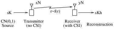
Suppose the distribution of the channel power gain is described by the probability density function (pdf) $f(\gamma)$, where $\gamma\triangleq\lvert{h}\rvert^{2}$ and $h\in\mathbb{C}$ is a realization of $H$. The receiver has perfect CSI but the transmitter has only channel distribution information (CDI), i.e., the transmitter knows the pdf $f(\gamma)$ but not its instantaneous realization. The channel is modeled by a quasi-static block fading process: $H$ is realized iid at the onset of each fading block and remains unchanged over the block duration. We assume decoding at the receiver is delay-limited; namely, delay constraints preclude coding across fading blocks but dictate that the receiver decodes at the end of each block. Hence the channel is non-ergodic.

Suppose each fading block spans $N$ channel uses, over which the transmitter describes $K$ of the source symbols. We define the bandwidth ratio as $b\triangleq N/K$, which relates the number of channel uses per source symbol. At the transmitter there is a power constraint on the transmit signal $\mathrm{E}\bigl[\lvert{x}\rvert^{2}\bigr]\leq P$, where the expectation is taken over repeated channel uses over the duration of each fading block. We assume a short-term power constraint and do not consider power allocation across fading blocks. We assume $K$ is large enough to consider the source as ergodic, and $N$ is large enough to design codes that achieve the instantaneous channel capacity of a given fading state with negligible probability of error.

At the receiver, the channel output $y$ is used to reconstruct an estimate $\hat{s}$ of the source. The distortion $D$ is measured by the mean squared error $\mathrm{E}[(s-\hat{s})^{2}]$ of the estimator, where the expectation is taken over the $K$-sequence of source symbols and the noise distribution. The instantaneous distortion of the reconstruction depends on the fading realization of the channel; we are interested in minimizing the expected distortion $\mathrm{E}_{H}[D]$, where the expectation is over the fading distribution.

We build upon the power allocation framework derived in [18], and first assume the fading distribution has $M$ discrete states: the channel power gain realization is $\gamma_{i}$ with probability $p_{i}$, for $i=1,\dotsc,M$, as depicted in Fig. 2. Accordingly there are $M$ virtual receivers and the transmitter sends the sum of $M$ layers of codewords. Let layer $i$ denote the layer of codeword intended for virtual receiver $i$, and we order the layers as $\gamma_{M}>\dotsb>\gamma_{1}\geq 0$. We refer to layer $M$ as the highest layer and layer 1 as the lowest layer. Each layer successively refines the description of the source $s$ from the layer below it, and the codewords in different layers are independent. Let $P_{i}$ be the transmit power allocated to layer $i$, then the transmit symbol $x$ can be written as

where $x_{1},\dotsc,x_{M}$ are iid ZMCSCG random variables with unit variance. Suppose the layers are evenly spaced, with $\gamma_{i+1}-\gamma_{i}=\Delta\gamma$. In Section IV we consider the limiting process as $\Delta\gamma\rightarrow 0$ to obtain the power distribution:

where for discrete layers the power allocation $P_{i}$ is referenced by the integer layer index $i$, while the continuous power distribution $\rho(\gamma)$ is indexed by the channel power gain $\gamma$.

With successive decoding [20], each virtual receiver first decodes and cancels the lower layers before decoding its own layer; the undecodable higher layers are treated as noise. Thus the rate $R_{i}$ intended for virtual receiver $i$ is

where the term $\gamma_{i}\sum_{j=i+1}^{M}P_{j}$ represents the interference power from the higher layers. Suppose $\gamma_{k}$ is the realized channel power gain, then the original receiver can decode layer $k$ and all the layers below it. Hence the realized rate $R_{\rlz}(k)$ at the original receiver is $R_{1}+\dotsb+R_{k}$.

From the rate distortion function of a complex Gaussian source [20], the mean squared distortion is $2^{-bR}$ when the source is described at a rate of $bR$ per symbol. Thus the realized distortion $D_{\rlz}(k)$ of the reconstructed source $\hat{s}$ is

where the last equality follows from successive refinability [14, 15]. The expected distortion $\mathrm{E}_{H}[D]$ is obtained by averaging over the fading distribution:

where $T_{i}$ represents the cumulative power in layers $i$ and above: $T_{i}\triangleq\sum_{j=i}^{M}P_{j}$, for $i=1,\dotsc,M$; $T_{M+1}\triangleq 0$. In the next section we derive the optimal cumulative power allocation $T_{2}^{*},\dotsc,T_{M}^{*}$ to find the minimum expected distortion $\mathrm{E}_{H}[D]^{*}$.

To derive the minimum expected distortion, we factor the sum of cumulative products in (5) and rewrite the expression as a set of recurrence relations:

where $i$ runs from $M-1$ down to 1. The term $D_{i}^{*}$ can be interpreted as the cumulative distortion from layers $i$ and above, with $D_{1}^{*}$ equal to the minimum expected distortion $\mathrm{E}_{H}[D]^{*}$. Note that $D_{i}$ depends on only two adjacent power allocation variables $T_{i}$ and $T_{i+1}$; therefore, in each recurrence step $i$ in (7), we solve for the optimal $T_{i+1}^{*}$ in terms of $T_{i}$.

Specifically, consider the optimal power allocation between layer $\gamma$ and its lower layer $\gamma-\Delta\gamma$ as shown in Fig. 3. Let $T(\gamma-\Delta\gamma)$ denote the available transmit power for layers $\gamma-\Delta\gamma$ and above, of which $T(\gamma)$ is allocated to layers $\gamma$ and above; the remaining power $T(\gamma)-T(\gamma-\Delta\gamma)$ is allocated to layer $\gamma-\Delta\gamma$. Under optimal power allocation, it is shown in [18] that the cumulative distortion from layers $\gamma$ and above can be written in the form:

where $W(\gamma)$ is interpreted as an equivalent probability weight summarizing the aggregate effect of the layers $\gamma$ and above. For the lower layer in Fig. 3, $f(\gamma)\Delta\gamma$ represents the probability that layer $\gamma-\Delta\gamma$ is realized.

In the next recurrence step as prescribed by (7), the cumulative distortion for the lower layer is

We solve the minimization by forming the Lagrangian:

The Karush-Kuhn-Tucker (KKT) conditions stipulate that the gradient of the Lagrangian vanishes at the optimal power allocation $T^{*}(\gamma)$, which leads to the solution:

where

We assume there is a region of $\gamma$ where the cumulative power allocation is not constrained by the power available from the lower layers, i.e., $U(\gamma)\leq U(\gamma-\Delta\gamma)$ and $U(\gamma)\leq P$. In this region the optimal power allocation $T^{*}(\gamma)$ is given by the unconstrained minimizer $U(\gamma)$ in (12a). In the solution to $U(\gamma)$ we need to verify that $U(\gamma)$ is non-increasing in this region, which corresponds to the power distribution $\rho^{*}(\gamma)$ being non-negative. With the substitution of the unconstrained cumulative power allocation $U(\gamma)$ in (10), the cumulative distortion at layer $\gamma-\Delta\gamma$ becomes:

which is of the form in (8) if we define $W(\gamma-\Delta\gamma)$ by the recurrence equation:

Next we consider the limiting process as the spacing between the layers condenses. In the limit of $\Delta\gamma$ approaching zero, the recurrence equations (14), (15) become differential equations. The optimal power distribution $\rho^{*}(\gamma)$ is given by the derivative of the cumulative power allocation:

where $T^{*}(\gamma)$ is described by solutions in three regions:

In region (17a) when $\gamma>\gamma_{o}$, corresponding to cases (12a) and (13a), no power is allocated to the layers and (15) simplifies to $W(\gamma)=1-F(\gamma)$, where $F(\gamma)\triangleq\int_{0}^{\gamma}f(s)\,ds$ is the cumulative distribution function (cdf) of the channel power gain. The boundary $\gamma_{0}$ is defined by the condition in (13a) which satisfies:

Under Rayleigh fading when $f(\gamma)=\bar{\gamma}^{-1}e^{-\gamma/\bar{\gamma}}$, where $\bar{\gamma}$ is the expected channel power gain, (18) evaluates to $\gamma_{o}=\bar{\gamma}$. For other fading distributions, $\gamma_{o}$ may be computed numerically.

In region (17b) when $\gamma_{P}\leq\gamma\leq\gamma_{o}$, corresponding to cases (12a) and (13b), the optimal power distribution is described by a set of differential equations. We apply the first order binomial expansion $(1+\Delta\gamma)^{b}\cong 1+b\Delta\gamma$, and (15) becomes:

which we substitute in (13b) to obtain:

Hence $U(\gamma)$ is described by a first order linear differential equation. With the initial condition $U(\gamma_{o})=0$, its solution is given by

and condition (12b) in the lowest active layer becomes the boundary condition $U(\gamma_{P})=P$. In [19], the power distribution in (22) is derived using the calculus of variations method.

Similarly, as $\Delta\gamma\rightarrow 0$, the evolution of the expected distortion in (14) becomes:

which is again a first order linear differential equation. With the initial condition $D(\gamma_{o})=W(\gamma_{o})=\gamma_{o}f(\gamma_{o})$, its solution is given by

Finally, in region (17c) when $\gamma<\gamma_{P}$, corresponding to case (12b), the transmit power $P$ has been exhausted, and no power is allocated to the remaining layers. Hence the minimum expected distortion is

where the last equality follows from when $\gamma<\gamma_{P}$ in region (17c), $\rho^{*}(\gamma)=0$ and $D(\gamma)=\int_{\gamma}^{\gamma_{P}}f(s)\,ds+D(\gamma_{P})$.

In this section we consider the optimal power distribution and the minimum expected distortion when the wireless channel undergoes Rayleigh fading with a diversity order of $L$ from the realization of independent fading paths. Specifically, we assume the fading channel is characterized by the Erlang distribution:

which corresponds to the average of $L$ iid channel power gains, each under Rayleigh fading with an expected value of $\bar{\gamma}$. The $L$-diversity system may be realized by having $L$ transmit antennas using isotropic inputs, by relaxing the decode delay constraint over $L$ fading blocks, or by having $L$ receive antennas under maximal-ratio combining when the power gain of each antenna is normalized by $1/L$.

Fig. 4 shows the optimal power distribution $\rho^{*}(\gamma)$, which is concentrated over a range of active layers. A higher SNR $P$ or a larger bandwidth ratio $b$ extends the span of the active layers further into the lower layers but the upper boundary $\gamma_{o}$ remains unperturbed. It can be observed that a smaller bandwidth ratio $b$ reduces the spread of the power distribution. In fact, as $b$ approaches zero, the optimal power distribution that minimizes expected distortion converges to the power distribution that maximizes expected capacity. To show the connection, we take the limit in the distortion-minimizing cumulative power distribution in (22):

which is equal to the capacity-maximizing cumulative power distribution as derived in [3]. Essentially, from the first order expansion $e^{b}\cong 1+b$ for small $b$, $\mathrm{E}_{H}[D]\cong 1-b\mathrm{E}_{H}[C]$ when the bandwidth ratio is small, where $\mathrm{E}_{H}[C]$ is the expected capacity in nats/s, and hence minimizing expected distortion becomes equivalent to maximizing expected capacity. For comparison, the capacity-maximizing power distribution is also plotted in Fig. 4. Note that the distortion-minimizing power distribution is more conservative, and it is more so as $b$ increases, as the allocation favors lower layers in contrast to the capacity-maximizing power distribution.

Fig. 5 shows the minimum expected distortion $\mathrm{E}_{H}[D]^{*}$ versus SNR for different diversity orders. With infinite diversity, the channel power gain becomes constant at $\bar{\gamma}$, and the distortion is given by

In the case when there is no diversity ($L=1$), a lower bound to the expected distortion is also plotted. The lower bound assumes the system has CSI at the transmitter (CSIT), which allows the transmitter to concentrate all power at the realized layer to achieve the expected distortion:

Note that at high SNR, the performance benefit from diversity exceeds that from CSIT, especially when the bandwidth ratio $b$ is large. In particular, in terms of the distortion exponent $\Delta$ [9], it is shown in [11] that in a MISO or SIMO channel, layered broadcast coding achieves:

where $L$ is the total diversity order from independent fading blocks and antennas. Moreover, the layered broadcast coding distortion exponent is shown to be optimal and CSIT does not improve $\Delta$, whereas diversity increases $\Delta$ up to a maximum as limited by the bandwidth ratio $b$.

We considered the problem of source-channel coding over a delay-limited fading channel without CSI at the transmitter, and derived the optimal power distribution that minimizes the end-to-end expected distortion in the layered broadcast coding transmission scheme with successive refinement. In the case when the channel undergoes Rayleigh fading with diversity order $L$, the optimal power distribution is congregated around the middle layers, and within this range the lower layers are assigned more power than the higher ones. As SNR increases, the power distribution of the higher layers remains unchanged, and the extra power is allocated to the idle lower layers. Furthermore, increasing the diversity $L$ concentrates the power distribution towards the expected channel power gain $\bar{\gamma}$, while a larger bandwidth ratio $b$ spreads the power distribution further into the lower layers. On the other hand, in the limit as $b$ tends to zero, the optimal power distribution that minimizes expected distortion converges to the power distribution that maximizes expected capacity. While the expected distortion can be improved by acquiring CSIT or increasing the diversity order, it is shown that at high SNR the performance benefit from diversity exceeds that from CSIT, especially when the bandwidth ratio $b$ is large.

References

- [1] T. M. Cover, “Broadcast channels,” IEEE Trans. Inform. Theory, vol. 18, no. 1, pp. 2–14, Jan. 1972.
- [2] S. Shamai (Shitz), “A broadcast strategy for the Gaussian slowly fading channel,” in Proc. IEEE Int. Symp. Inform. Theory, June 1997, p. 150.
- [3] S. Shamai (Shitz) and A. Steiner, “A broadcast approach for a single-user slowly fading MIMO channel,” IEEE Trans. Inform. Theory, vol. 49, no. 10, pp. 2617–2635, Oct. 2003.
- [4] T. J. Goblick, Jr., “Theoretical limitations on the transmission of data from analog sources,” IEEE Trans. Inform. Theory, vol. 11, no. 4, pp. 558–567, Oct. 1965.
- [5] M. Gastpar, B. Rimoldi, and M. Vetterli, “To code, or not to code: Lossy source-channel communication revisited,” IEEE Trans. Inform. Theory, vol. 49, no. 5, pp. 1147–1158, May 2003.
- [6] S. Shamai (Shitz), S. Verdú, and R. Zamir, “Systematic lossy source/channel coding,” IEEE Trans. Inform. Theory, vol. 44, no. 2, pp. 564–579, Mar. 1998.
- [7] U. Mittal and N. Phamdo, “Hybrid digital-analog (HDA) joint source-channel codes for broadcasting and robust communications,” IEEE Trans. Inform. Theory, vol. 48, no. 5, pp. 1082–1102, May 2002.
- [8] Z. Reznic, M. Feder, and R. Zamir, “Distortion bounds for broadcasting with bandwidth expansion,” IEEE Trans. Inform. Theory, vol. 52, no. 8, pp. 3778–3788, Aug. 2006.
- [9] J. N. Laneman, E. Martinian, G. W. Wornell, and J. G. Apostolopoulos, “Source-channel diversity for parallel channels,” IEEE Trans. Inform. Theory, vol. 51, no. 10, pp. 3518–3539, Oct. 2005.
- [10] D. Gunduz and E. Erkip, “Source and channel coding for quasi-static fading channels,” in Proc. of Asilomar Conf. on Signals, Systems and Computers, Nov. 2005.
- [11] ——, “Joint source-channel codes for MIMO block fading channels,” IEEE Trans. Inform. Theory, submitted.
- [12] G. Caire and K. Narayanan, “On the SNR exponent of hybrid digital-analog space time coding,” in Proc. Allerton Conf. Commun., Contr., Comput., Oct. 2005.
- [13] F. Etemadi and H. Jafarkhani, “Optimal layered transmission over quasi-static fading channels,” in Proc. IEEE Int. Symp. Inform. Theory, July 2006, pp. 1051–1055.
- [14] W. H. R. Equitz and T. M. Cover, “Successive refinement of information,” IEEE Trans. Inform. Theory, vol. 37, no. 2, pp. 269–275, Mar. 1991.
- [15] B. Rimoldi, “Successive refinement of information: Characterization of the achievable rates,” IEEE Trans. Inform. Theory, vol. 40, no. 1, pp. 253–259, Jan. 1994.
- [16] S. Sesia, G. Caire, and G. Vivier, “Lossy transmission over slow-fading AWGN channels: a comparison of progressive, superposition and hybrid approaches,” in Proc. IEEE Int. Symp. Inform. Theory, Sept. 2005, pp. 224–228.
- [17] K. E. Zachariadis, M. L. Honig, and A. K. Katsaggelos, “Source fidelity over fading channels: Erasure codes versus scalable codes,” in Proc. IEEE Globecom Conf., vol. 5, Nov. 2005, pp. 2558–2562.
- [18] C. T. K. Ng, D. Gündüz, A. J. Goldsmith, and E. Erkip, “Recursive power allocation in Gaussian layered broadcast coding with successive refinement,” to appear at IEEE Internat. Conf. Commun., June 2007.
- [19] C. Tian, A. Steiner, S. Shamai (Shitz), and S. Diggavi, “Expected distortion for Gaussian source with a broadcast transmission strategy over a fading channel,” submitted to IEEE Inform. Theory Workshop, Sept. 2007.
- [20] T. M. Cover and J. A. Thomas, Elements of Information Theory. Wiley-Interscience, 1991.