Joint Universal Lossy Coding and Identification
of Stationary Mixing Sources

A universal source coding scheme is one that performs asymptotically optimally for all sources within a given class. Intuition suggests that a good universal coder should acquire a probabilistic model of the source from a sufficiently long data sequence and operate based on this model. For lossless codes, this intuition has been made rigorous by Rissanen [1]: the data are encoded via a two-part code which comprises (1) a suitably quantized maximum-likelihood estimate of the source parameters, and (2) an encoding of the data with the code optimized for the acquired model. The redundancy of this scheme converges to zero as $k\log n/n$, where $n$ is the block length and $k$ is the dimension of the parameter space.

Recently we have extended Rissanen’s ideas to lossy block coding of finitely parametrized continuous-alphabet i.i.d. sources with bounded parameter spaces [2, 3]. We have shown that, under appropriate regularity conditions, there exist joint universal schemes for lossy coding and source identification whose distortion redundancy and source estimation fidelity both converge to zero as $O\big(\sqrt{\log n/n}\big)$ as the block length $n$ tends to infinity. The code operates by coding each block with the code matched to the parameters estimated from the preceding block. Moreover, the constant hidden in the $O(\cdot)$ notation increases with the “richness” of the model class, as measured by the Vapnik–Chervonenkis (VC) dimension [4, 5] of a certain class of decision regions in the source alphabet.

The main limitation of the results of [2, 3] is the i.i.d. assumption, which excludes such practically relevant model classes as autoregressive sources or Markov and hidden Markov processes. Furthermore, the assumption of a bounded parameter space may not be always justified. In this paper we relax both of these assumptions. Because the parameter space is not bounded, we have to use variable-rate codes with countably infinite codebooks, whose performance is naturally quantified by Lagrangians [6, 7]. We show that, under certain regularity conditions, there are universal schemes for joint lossy source coding and modeling such that, as the block length $n$ tends to infinity, both the Lagrangian redundancy relative to the best variable-rate code at each block length and the source estimation fidelity at the decoder converge to zero as $O(\sqrt{V_{n}\log n/n})$, where $V_{n}$ is the VC dimension of a certain class of decision regions induced by the collection of all $n$-dimensional marginals of the source process distributions.

The key novel feature of our scheme is that, unlike most existing schemes for universal lossy coding, which rely on implicit identification of the active source, it learns an explicit probabilistic model. Moreover, our results clearly show that the “price of universality” of a modeling-based compression scheme grows with the combinatorial richness of the underlying model class, as captured by the VC dimension sequence $\{V_{n}\}$. The richer the model class, the harder it is to learn, which in turn affects the compression performance because we use the source parameters learned from past data in deciding how to encode the current block. These insights may prove useful in such settings as digital forensics or adaptive control under communication constraints, where trade-offs between the quality of parameter estimation and compression performance are of central importance.

Let $\boldsymbol{X}=\{X_{i}\}_{i\in\mathbb{Z}}$ be a stationary, ergodic source with alphabet ${\cal X}$. All alphabets are assumed to be Polish spaces equipped with their Borel $\sigma$-fields. We adopt the usual setting of universal source coding: the process distribution of $\boldsymbol{X}$ is not known exactly, apart from being a member of some indexed class $\{P_{\theta}:\theta\in\Lambda\}$. We assume that the parameter space $\Lambda$ is an open subset of $\mathbb{R}^{k}$ with nonempty interior. We also assume that there exists a $\sigma$-finite measure $\mu$ on ${\cal X}$, such that for every $\theta\in\Lambda$ the $n$-dimensional marginals $P^{n}_{\theta}$ of $P_{\theta}$ are absolutely continuous with respect to (w.r.t.) the product measure $\mu^{n}$, for all $n$, denoting the corresponding densities $dP^{n}_{\theta}/d\mu^{n}$ by $p^{n}_{\theta}$.

We wish to code $\boldsymbol{X}$ into a reproduction process $\widehat{\boldsymbol{X}}=\{\widehat{X}_{i}\}_{i\in\mathbb{Z}}$ with alphabet $\widehat{\cal X}$ by means of a finite-memory variable-rate lossy block code (vector quantizer). Such a code with block length $n$ and memory length $m$ [an $(n,m)$-block code, for short] is a pair $C^{n,m}=(f,\varphi)$, where $f:{\cal X}^{n}\times{\cal X}^{m}\rightarrow{\cal S}$ is the encoder, $\varphi:{\cal S}\rightarrow\widehat{\cal X}^{n}$ is the decoder, and ${\cal S}\subseteq\{0,1\}^{*}$ is a finite or countable collection of binary strings satisfying the prefix condition. The mapping of $\boldsymbol{X}$ into $\widehat{\boldsymbol{X}}$ is defined by $\widehat{X}^{n(k+1)}_{nk+1}=\varphi(f(X^{n(k+1)}_{nk+1},X^{nk}_{nk-m+1}))$, $k\in\mathbb{Z}$, where $X^{j}_{i}\stackrel{{\scriptstyle\scriptscriptstyle\triangle}}{{=}}(X_{i},X_{i+1},\ldots,X_{j})$, $i<j$. Thus, the encoding is done in blocks of length $n$, but the encoder is also allowed to view the $m$ source symbols immediately preceding the current $n$-block. Abusing notation, we shall denote by $C^{n,m}$ both the composition $\varphi\circ f$ and the pair $(f,\varphi)$; when $m=0$, we shall use a more compact notation $C^{n}$ and say “$n$-block code.”

Let $\rho:{\cal X}\times\widehat{\cal X}\rightarrow\mathbb{R}^{+}$ be a measurable single-letter distortion function; $\rho_{n}(x^{n},\widehat{x}^{n})=n^{-1}\sum^{n}_{i=1}\rho(x_{i},\widehat{x}_{i})$ is the per-letter distortion due to reproducing $x^{n}\in{\cal X}^{n}$ by $\widehat{x}^{n}\in\widehat{\cal X}^{n}$. We assume that $\rho$ is a metric on ${\cal X}\cup\widehat{\cal X}$, bounded from above by some $\rho_{\max}<\infty$. Suppose $\boldsymbol{X}\sim P_{\theta}$. Associated with the code $C^{n,m}$ are its expected distortion $D_{\theta}(C^{n,m})\stackrel{{\scriptstyle\scriptscriptstyle\triangle}}{{=}}\operatorname{{\mathbb{E}}}_{\theta}\{\rho_{n}(X^{n}_{1},\widehat{X}^{n}_{1})\}$ and its expected rate $R_{\theta}(C^{n,m})\stackrel{{\scriptstyle\scriptscriptstyle\triangle}}{{=}}\operatorname{{\mathbb{E}}}_{\theta}\{\ell_{n}(f(X^{n}_{1},X^{0}_{-m+1}))\}$, where, for a binary string $s$, $\ell_{n}(s)$ is its length in bits, normalized by $n$. When working with variable-rate quantizers, it is convenient [6, 7] to absorb the distortion and the rate into a single performance measure, the Lagrangian $L_{\theta}(C^{n,m},\lambda)\stackrel{{\scriptstyle\scriptscriptstyle\triangle}}{{=}}D_{\theta}(C^{n,m})+\lambda R_{\theta}(C^{n,m})$, where $\lambda>0$ is the Lagrange multiplier which controls the distortion-rate trade-off. The optimal Lagrangian performance achievable on $P_{\theta}$ by any zero-memory variable-rate quantizer with block length $n$ is given by the $n$th-order operational distortion-rate Lagrangian $\widehat{L}^{n}_{\theta}(\lambda)\stackrel{{\scriptstyle\scriptscriptstyle\triangle}}{{=}}\inf_{C^{n}}L_{\theta}(C^{n},\lambda)$ [6]. Allowing the codes to have nonzero memory does not improve optimal performance, because we can use memoryless nearest-neighbor encoders to convert any $(n,m)$-block code into an $n$-block code without increasing the Lagrangian. Thus, $\widehat{L}^{n}_{\theta}(\lambda)=\inf_{m}\inf_{C^{n,m}}L_{\theta}(C^{n,m},\lambda)$, where the infimum is over all memory lengths $m$ and all $(n,m)$-block codes $C^{n,m}$, for a fixed block length $n$. Because each $P_{\theta}$ is ergodic, $\widehat{L}^{n}_{\theta}(\lambda)$ converges, as $n\to\infty$, to the distortion-rate Lagrangian $L_{\theta}(\lambda)\stackrel{{\scriptstyle\scriptscriptstyle\triangle}}{{=}}\min_{R}\Big(D_{\theta}(R)+\lambda R\Big)$, where $D_{\theta}(R)$ is the Shannon distortion-rate function of $P_{\theta}$ [6].

In this section we state our result on universal schemes for joint lossy compression and identification of stationary sources satisfying certain regularity conditions. We wish to design a sequence of variable-rate vector quantizers, such that the decoder can reliably reconstruct the source sequence $\boldsymbol{X}$ and reliably identify the active source in an asymptotically optimal manner for all $\theta\in\Lambda$. The identification performance will be judged in terms of the variational distance, which for any two probability measures $P,Q$ on a measurable space $({\cal Z},{\cal A})$ is defined by $d(P,Q)\stackrel{{\scriptstyle\scriptscriptstyle\triangle}}{{=}}2\sup_{A\in{\cal A}}|P(A)-Q(A)|$. Denoting by $p$ and $q$ the respective densities of $P$ and $Q$ w.r.t. a dominating measure $\nu$, we can also write $d(P,Q)=\int_{\cal X}|p(z)-q(z)|d\nu(z)$. The set of all $Q$ satisfying $d(P,Q)\leq\delta$ for a given $P$ is called the variational ball of radius $\delta$ around $P$.

Our first condition ensures that each source in the class is sufficiently close to an i.i.d. source, in an asymptotic sense. Define the $k$th $\beta$-mixing coefficient of $P_{\theta}$ [5] by

where $\sigma(X^{0}_{-\infty},X^{\infty}_{k})$ is the $\sigma$-field generated by $\{X_{i}\}_{i\leq 0}$ and $\{X_{i}\}_{i\geq k}$, and $P^{-}_{\theta}$ and $P^{+}_{\theta}$ are the marginal distributions of $\{X_{i}\}_{i\leq 0}$ and $\{X_{i}\}_{i>0}$, respectively. An i.i.d. source has $\beta(k)\equiv 0,\forall k$; if $\beta(k)\stackrel{{\scriptstyle k\to\infty}}{{\longrightarrow}}0$, the source is called $\beta$-mixing.

The second condition ensures that the parametrization of the sources is sufficiently smooth.

This condition is met, for instance, if the asymptotic Fisher information matrix $I(\theta)$ exists for all $\theta\in\Lambda$ (under some technical assumptions on the densities $p^{n}_{\theta}$). It guarantees that, for every sequence $\{\delta_{n}\}_{n\in\mathbb{N}}$ of positive reals satisfying $\delta_{n}\to 0,\sqrt{n}\delta_{n}\to 0$ as $n\to\infty$, and for every sequence $\{\theta_{n}\}_{n\in\mathbb{N}}$ in $\Lambda$ satisfying $\|\theta_{n}-\theta\|<\delta_{n}$ for a given $\theta\in\Lambda$, we have $d_{n}(\theta_{n},\theta)\to 0$ as $n\to\infty$.

Finally, we impose a learnability condition. To state it we need some facts on Vapnik–Chervonenkis classes (see, e.g., [4, 5]). Let $({\cal Z},{\cal A})$ be a measurable space. Given a collection ${\cal C}$ of measurable subsets of ${\cal Z}$, its Vapnik-Chervonenkis (VC) dimension ${\sf V}({\cal C})$ is defined as the largest integer $n$ for which

if (1) holds for all $n$, then ${\sf V}({\cal C})=\infty$. If ${\sf V}({\cal C})<\infty$, we say that ${\cal C}$ is a VC class. The Vapnik–Chervonenkis inequalities are finite-sample bounds on uniform deviations of probabilities of events in a VC class from their relative frequencies: if $X^{n}=(X_{1},\cdots,X_{n})$ is an i.i.d. sample from a probability measure $P$ on $({\cal Z},{\cal A})$, and if ${\cal C}$ is a VC class with ${\sf V}({\cal C})\geq 2$, then

where $c>0$ is a universal constant¹¹ 1 Using more refined techniques, the $c\sqrt{{\sf V}({\cal C})\log n/n}$ bound can be improved to $c^{\prime}\sqrt{{\sf V}({\cal C})/n}$, where $c^{\prime}$ is another constant. However, $c^{\prime}$ is much larger than $c$, so any benefit of the new bound shows only for “impractically” large values of $n$., $P_{X^{n}}$ is the empirical distribution of $X^{n}$, and the probabilities and expectations are w.r.t. the product measure $P^{n}$ on $({\cal Z}^{n},{\cal A}^{n})$.

That is, for each $n,\theta$ the code $C^{n,m_{n}}_{*}$, which is independent of $\theta$, performs almost as well as the best finite-memory quantizer with block length $n$ that can be designed with full knowledge of $P^{n}_{\theta}$. Thus, as far as compression goes, our scheme can compete with all finite-memory variable-rate quantizers, with the additional bonus of allowing the decoder to identify the active source in an asymptotically optimal manner. Recalling the discussion of Lagrangian optimality in Section II, we see that Theorem 1 immediately implies the following:

We assume throughout that the “true” source is $P_{\theta_{0}}$ for some $\theta_{0}\in\Lambda$. Our code operates as follows. Suppose that both the encoder and the decoder have access to a countably infinite “database” $\boldsymbol{c}=\{\theta(i)\}_{i\in\mathbb{N}}\subset\Lambda$. Using Elias’ universal representation of the integers [8], we can associate to each $\theta(i)$ a unique binary string $s(i)$ with $\ell(s(i))=\log i+O(\log\log i)$ bits. Suppose also that for each $n,\theta$ there exists a zero-memory $n$-block code $C^{n}_{\theta}=(f_{\theta},\varphi_{\theta})$ that achieves the $n$th-order Lagrangian optimum for $P_{\theta}$: $L_{\theta}(C^{n}_{\theta},\lambda)=\widehat{L}^{n}_{\theta}(\lambda)$. The encoding of $X^{n}_{1}$ into $\widehat{X}^{n}_{1}$ is done as follows:

1. 1.

   The encoder estimates $P^{n}_{\theta_{0}}$ from the $m_{n}$-block $X^{0}_{-m_{n}+1}$ as $P^{n}_{\widetilde{\theta}}$, where $\widetilde{\theta}=\widetilde{\theta}(X^{0}_{-m_{n}+1})$.

2. 2.

   The encoder then computes the waiting time

   $$T_{n}\stackrel{{\scriptstyle\scriptscriptstyle\triangle}}{{=}}\inf\big\{i\geq 1:d_{n}\big(\theta(i),\widetilde{\theta}(X^{0}_{-m_{n}+1})\big)\leq\sqrt{n}\delta_{n}\big\},\vskip-4.0pt$$

   with the standard convention that the infimum of the empty set is equal to $+\infty$; $\{\delta_{n}\}$ is a sequence of positive reals to be specified later.

3. 3.

   If $T_{n}<+\infty$, the encoder sets $\widehat{\theta}=\theta(T_{n})$; otherwise, the encoder sets $\widehat{\theta}=\theta(1)$ (or some other default $\theta$).

4. 4.

   The description of $X^{n}_{1}$ is a concatenation of three binary strings: (i) a 1-bit flag $b$ to tell whether $T_{n}$ is finite $(b=0)$ or infinite $(b=1)$; (ii) a binary string $s_{1}$ which is equal to $s(T_{n})$ if $T_{n}<+\infty$ or is empty if $T_{n}=+\infty$; (iii) $s_{2}=f_{\widehat{\theta}}(X^{n}_{1})$. The string $\widetilde{s}=bs_{1}$ is the first-stage description, while $s_{2}$ is the second-stage description.

The decoder receives $bs_{1}s_{2}$, determines $\widehat{\theta}$ from $\widetilde{s}$, and produces $\widehat{X}^{n}_{1}=\varphi_{\widehat{\theta}}(s)$. If $b=0$ (which, as we shall show, will happen eventually a.s.), then $P^{n}_{\widehat{\theta}}$ is in the variational ball of radius $\sqrt{n}\delta_{n}$ around the estimated $P^{n}_{\widetilde{\theta}}$. If the latter is a good estimate, i.e., $d_{n}(\theta_{0},\widetilde{\theta})\stackrel{{\scriptstyle{\rm a.s.}}}{{\to}}0$ as $n\to\infty$, then the decoder’s estimate of $P^{n}_{\theta_{0}}$ is only slightly worse. Moreover, the a.s. convergence of $d_{n}(\theta_{0},\widehat{\theta})$ to zero as $n\to\infty$ implies that the performance of $C^{n}_{\widehat{\theta}}$ on $P_{\theta_{0}}$ is close to the optimum $L_{\theta_{0}}(C^{n}_{\theta_{0}},\lambda)\equiv\widehat{L}^{n}_{\theta_{0}}(\lambda)$.

Formally, the code $C^{n,m_{n}}_{*}$ is comprised by the following maps: (1) the parameter estimator $\widetilde{\theta}:{\cal X}^{m_{n}}\rightarrow\Lambda$; (2) the parameter encoder $\widetilde{g}:\Lambda\rightarrow\widetilde{{\cal S}}$, where $\widetilde{{\cal S}}=\{0s(i)\}_{i\in\mathbb{N}}\cup\{1\}$; (3) the parameter decoder $\widetilde{\psi}:\widetilde{{\cal S}}\rightarrow\Lambda$. Let $\widetilde{f}$ denote the composition $\widetilde{g}\circ\widetilde{\theta}$ of the parameter estimator and the parameter encoder, which we refer to as the first-stage encoder, and let $\widehat{\theta}$ denote the composition $\widetilde{\psi}\circ\widetilde{f}$ of the parameter decoder and the first-stage encoder. The decoder $\widetilde{\psi}$ is the first-stage decoder. The collection $\{C^{n}_{\theta}:\theta\in\Lambda\}$ defines the second-stage codes. The encoder $f_{*}:{\cal X}^{n}\times{\cal X}^{m_{n}}\rightarrow\widetilde{{\cal S}}\times{\cal S}$ and the decoder $\varphi_{*}:\widetilde{{\cal S}}\times{\cal S}\rightarrow\widehat{\cal X}^{n}$ of $C^{n,m_{n}}_{*}$ are defined as $f_{*}(X^{n}_{1},X^{0}_{-m_{n}+1})=\widetilde{f}(X^{0}_{-m_{n}+1})f_{\widehat{\theta}(X^{0}_{-m_{n}+1})}(X^{n}_{1})$ and $\varphi_{*}(\widetilde{s}s)=\varphi_{\widetilde{\psi}(\widetilde{s})}(s)$ for all $s\in{\cal S},\widetilde{s}\in\widetilde{{\cal S}}$, respectively.

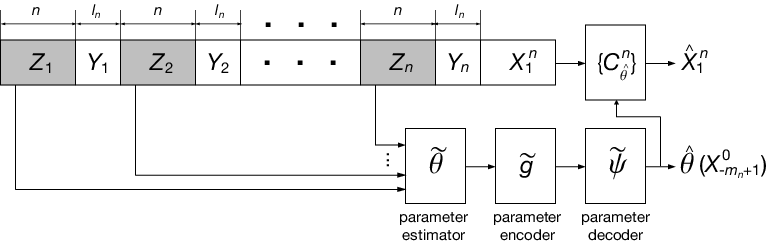
To assess the performance of the code, introduce the functions $g(x^{n},y^{m_{n}})=\rho_{n}(x^{n},C^{n}_{\widehat{\theta}(y^{m_{n}})}(x^{n}))+\lambda\ell_{n}(f_{\widehat{\theta}(y^{m_{n}})}(x^{n}))$ and $h(y^{m_{n}})=\ell_{n}(\widetilde{f}(y^{m_{n}}))$. Then $h(X^{0}_{-m_{n}+1})$ is the normalized length of the first-stage description, while $g(X^{n}_{1},X^{0}_{-m_{n}+1})$ is the instantaneous Lagrangian performance of the corresponding second-stage code. The expected Lagrangian performance of our code is

We prove the theorem by showing that, with proper choices for the memory length $m_{n}$, the “database” $\boldsymbol{c}$, the parameter estimator $\widetilde{\theta}$, and the sequence $\{\delta_{n}\}$, we can ensure that $\operatorname{{\mathbb{E}}}_{\theta_{0}}h(X^{0}_{-m_{n}+1})=O(k\log n/n)+O(\log\log n/n)+o(1)$, $\operatorname{{\mathbb{E}}}_{\theta_{0}}g(X^{n}_{1},X^{0}_{-m_{n}+1})=\widehat{L}^{n}_{\theta}(\lambda)+O(\sqrt{V_{n}\log n/n})$, and $d_{n}(\theta_{0},\widehat{\theta}(X^{0}_{-m_{n}+1}))=O(\sqrt{V_{n}\log n/n})$ $P_{\theta_{0}}$-almost surely.

Here, we present three examples of parametric families satisfying the conditions of Theorem 1 and thus admitting joint universal lossy coding and identification schemes. The following result [5] will be used throughout: Let ${\cal C}=\{A_{\xi}:\xi\in\mathbb{R}^{N}\}$ be a collection of measurable subsets of $\mathbb{R}^{d}$, such that $A_{\xi}=\{z\in\mathbb{R}^{d}:\Pi(z,\xi)>0\}$ for all $\xi$, where for each $z\in\mathbb{R}^{d}$, $\Pi(z,\cdot)$ is a polynomial of degree $s$ in the components of $\xi$. Then ${\cal C}$ is a VC class with ${\sf V}({\cal C})\leq 2N\log(4es)$.

References

- [1] J. Rissanen, “Universal coding, information, prediction, and estimation,” IEEE Trans. Inform. Theory, vol. IT-30, no. 4, pp. 629–636, July 1984.
- [2] M. Raginsky, “Joint fixed-rate universal lossy coding and identification of continuous-alphabet memoryless sources,” IEEE Trans. Inform. Theory, 2005, submitted.