Optimum Linear LLR Calculation for Iterative Decoding on Fading Channels

Iterative decoding has received much attention in the past decade due to its exemplary performance. There have been many advances in iterative decoding techniques and it has been shown that using graphical codes such as low-density parity-check (LDPC) codes [1] and turbo codes [2] associated with iterative decoding, the Shannon limit on many channels (e.g., additive white Gaussian noise channel) can be approached [3]. Therefore, these codes have also been proposed for wireless fading channels [4].

Application of LDPC codes on Rayleigh fading channel is pioneered in [4], where a detailed study of performance and code design is conducted. This work is later extended to complex fading channels [5], to Rician fading channels [6], and also to Rayleigh block fading channels [7]. The application of turbo codes on Rayleigh fading channels is also studied in [8].

For soft iterative decoding, log-likelihood ratios (LLRs) at the output of the channel are calculated. The process of computing LLRs depends on whether or not a perfect knowledge of the channel parameters exists at the receiver. The capacity of the fading channel is also affected with the availability of channel parameters at the receiver [8].

An uncorrelated fading channel can be modeled with a fading gain $r$ and an additive Gaussian noise $n\sim\mathcal{N}(0,\sigma_{n}^{2})$. When $r$ is known at the receiver as a perfect side information (SI), LLRs are linear functions of the channel output [4]. Exact LLR computation depends on a perfect knowledge of $\sigma_{n}$ at the receiver.

In order to have SI at the receiver, channel estimation techniques must be used. These techniques increase the complexity of the system, can cause a significant overhead, and are themselves subject to imperfections. For high throughput wireless applications, the receiver may not be able to handle the extra complexity or overhead. This paper provides an alternative solution which does not require channel estimation, yet provides better performance compared to the existing solutions that use fixed fading gain estimates in the decoder.

With no SI available at the receiver, LLRs are complicated functions of the channel output [9] and depend on the probability density function (pdf) of $r$. An approximate LLR, however, can be computed as a linear function of the channel output [9]. The coefficient of this linear function depends on a fixed estimate $\hat{r}$ of the channel fading gain and a knowledge of $\sigma_{n}$. Previous work assume that $\sigma_{n}$ is known and use the expected value of $r$ for $\hat{r}$ [4, 8]. While the expected value of the fading gain is the minimum mean square error estimation of $r$, it is not guaranteed that this choice provides the optimum performance in the decoder.

In a general setup (which includes famous fading channel models such as uncorrelated Rayleigh and Rician fading channels), we propose the following question: Assume that the pdf of $r$ is known at the receiver, but the channel fading gain is not. Also assume that LLRs are to be computed as linear functions of the channel output. What linear approximation provides the optimum decoding performance?

This question is studied in this paper and the following contributions are made: (1) When $\sigma_{n}$ is known, we find a linear LLR approximation which allows for the maximum achievable code rate on the channel. We prove that the optimum linear approximation is unique and we observe that, on a Rayleigh fading channel, it closely approaches the capacity under true LLR calculation. This solution can significantly outperform LLR calculation based on the expected value of $r$. We also design irregular LDPC codes which approach this maximum achievable rate. (2) When neither $r$ nor $\sigma_{n}$ is known at the receiver, we propose a linear LLR calculation technique which guarantees the convergence of the decoder over the widest possible range of $\sigma_{n}$. The performance of this solution is almost identical to the case that $\sigma_{n}$ is perfectly known. We design appropriate irregular LDPC codes for this case too.

This paper is organized as follows. Section II reviews some preliminaries and studies the proposed approaches. Section III studies the problem when $\sigma_{n}$ is known to the receiver. Section IV extends our results to the case that $\sigma_{n}$ is unknown. Section V concludes the paper.

As mentioned before, when no SI is available at the receiver, one can calculate the LLRs linearly via (6) as an approximation to (4). The objective is to find the optimal linear approximation. Different measures of optimality can be considered. Existing work assumes that $\sigma_{n}$ is known and chooses $\hat{r}=\mathrm{E}[r]$. This choice of $\hat{r}$ is optimum in the sense of minimum mean square error $\mathrm{E}[|r-\hat{r}|^{2}]$. In this work, we find the linear approximation which gives a nearly consistent LLR pdf and results in the maximum achievable transmission rate on the channel. We call this linear approximation maximum-capacity linear-approximation (MCLA).

Different linear approximations result in different LLR distributions for $\hat{l}$. Each LLR distribution defines a corresponding $\hat{C}$ according to (9). Thus, the problem of finding the MCLA is simplified to finding a linear approximation whose corresponding LLR distribution maximizes the capacity $\hat{C}$.

Maximizing $\hat{C}$ requires a knowledge of $\sigma_{n}$ and pdf of $r$. These are needed for finding the pdf of $\hat{l}$ and thus optimizing its corresponding capacity. So, we first assume that these pieces of information are available. Later we generalize our results to the case that $\sigma_{n}$ is unknown. When $\sigma_{n}$ is known, without loss of generality we set $\hat{\sigma}_{n}=\sigma_{n}$ in (6) and we find the optimum choice of $\hat{r}$. Notice that with $\hat{r}$ one can adjust $\alpha$ and thus the pdf of $\hat{l}$ as needed.

MCLA maximizes a bound on the achievable transmission rate. To show that this optimization is meaningful in practice, we design irregular LDPC codes that approach this maximized capacity. More interestingly, we observe that the optimized $\hat{C}$ is extremely close to $C$ based on true LLR calculation.

MCLA is also expected to result in improved performance in iterative decoders. That is, for a fixed code, computing LLRs according to MCLA should improve BER performance. Our simulation results will support this claim, but the following two arguments can also be provided to justify this choice. (1) MCLA provides the maximum $\hat{C}$ and thus the maximum gap between the code rate $R$ and the capacity $\hat{C}$. Thus one expects improved BER performance. (2) Since $\hat{l}$ is not the true LLR, under any linear LLR calculation, $\hat{C}\leq C$. Under a good linear approximation, pdf of $\hat{l}$ is close to that of true LLRs and thus $\hat{C}$ is close to $C$. Hence, a minimized $C-\hat{C}$ (through maximizing $\hat{C}$) indicates a good LLR approximation.

As mentioned, our simulation results show that MCLA indeed improves the performance compared to existing work based on choosing $\hat{r}=\mathrm{E}[r]$. Moreover, though not rigorously proved, MCLA appears to be the optimum choice in terms of BER performance too. Thus, our proposed method is based on maximizing $\hat{C}$ over $\hat{r}$ for fixed $\hat{\sigma}_{n}$ and $\sigma_{n}$, and we define

The following theorem suggests that finding $\hat{r}_{\mathsf{opt}}$ can be done very efficiently.

Proof:

The above expression is negative since the term inside the expected value is always negative. Therefore, $\hat{C}$ is a concave function of $\hat{r}$ and there exists a unique maximum in $\hat{r}=\hat{r}_{\mathsf{opt}}$. This theorem is valid for any distribution of $r\geq 0$. $\blacksquare$

Maximizing $\hat{C}$, therefore, is a straightforward task because it is a one-variable convex-optimization problem and can be solved very efficiently by simple numerical techniques. Different $\hat{C}$ curves are depicted in Fig. 1 for some $\hat{r}$ and the case $\hat{\sigma}_{n}=\sigma_{n}$. Notice that $\hat{r}_{\mathsf{opt}}$ is not very sensitive to $\sigma_{n}$.

Fig. 2 shows that we can get very close to the channel capacity under MCLA. Simulations show that $\hat{r}=\mathrm{E}[r]$ can result in significant performance loss especially when the capacity or the code rate increases. This performance loss is about 0.24 dB in 0.5 bits/channel use to 0.92 dB in 0.75 bits/channel use.

The following two examples support our above mentioned results. In Example 1, we design an irregular LDPC code which approaches the capacity that is maximized by MCLA. Example 2 shows improved BER performance under MCLA.

Example 1: Consider an uncorrelated normalized Rayleigh fading channel with $\sigma_{n}=0.7436$. The channel capacity is 0.5 bits/channel use in the absence of SI and $\hat{C}=0.4999$ using $\hat{r}_{\mathsf{opt}}=0.6594$ (compare with $\mathrm{E}[r]=0.8862$). We design a code based on rate maximization under MCLA. We assume a fixed $\rho(x)=x^{8}$ and a maximum variable node degree $d_{v}$ of 30. Under MCLA and 11-bit decoding, and allowing a maximum of 300 iterations, the optimized code is given in Table I (Code1). The rate of the designed code is 0.4889. The designed code has almost approached $\hat{C}$ and also the capacity of the channel with no SI.

Example 2: To show that MCLA also improves the BER of the code, a $\mathcal{C}^{10000}(x^{2},x^{5})$ LDPC code is simulated on an uncorrelated normalized Rayleigh fading channel. Fig. 3 shows the BER of the code with and without SI at the receiver. When SI is not available and $\sigma_{n}$ is known, two cases have been plotted. One is when $\hat{\sigma}_{n}=\sigma_{n}$ and $\hat{r}=\mathrm{E}[r]$ and the other is under MCLA (i.e., $\hat{\sigma}_{n}=\sigma_{n}$ and $\hat{r}=\hat{r}_{\mathsf{opt}}$). The decoding threshold of the code is 4.06 dB with $\hat{r}=\mathrm{E}[r]$ and no SI, 3.82 dB under MCLA, and 3.06 dB with perfect SI. The figure shows considerable BER improvement under MCLA. We have chosen a (3,6)-regular LDPC code since most of its results exist in the literature. If a higher rate code (e.g., $R=3/4$) is used, the performance improvement increases.

Under MCLA, the pdf of $\hat{l}$ is a linear transformation of the pdf of $y$. In fact, $\alpha_{\mathsf{opt}}=2\frac{\hat{r}_{\mathsf{opt}}}{\sigma_{n}^{2}}$ would give the linear transformation whose associated capacity (given by (9)) is maximum. When $\sigma_{n}$ is unknown, the distribution of $y$ is not known at the receiver. Therefore, finding the optimum linear transform is somewhat meaningless. However, for any $\sigma_{n}$ one can find $\alpha_{\mathsf{opt}}$. Thus, $\alpha_{\mathsf{opt}}$ is a function of $\sigma_{n}$. It is also obvious from Theorem 1, that $\alpha_{\mathsf{opt}}$ is unique for each $\sigma_{n}$. Thus, $\alpha_{\mathsf{opt}}$ will be denoted as $\alpha_{\mathsf{opt}}(\sigma_{n})$ afterwards.

Since $\sigma_{n}$ is unknown, $\alpha_{\mathsf{opt}}(\sigma_{n})$ is also unknown. However, one can find $\alpha$ such that a given code has the widest range of convergence over changes of $\sigma_{n}$. This way, we ensure that the code is robust to the changes in the noise power (e.g. when the code is used in different channels with different noise powers).

The basic idea for finding such $\alpha$ is to maximize the achievable transmission rate at the highest noise standard deviation that the code can tolerate under MCLA. To do this, for a given code, we must find the largest $\sigma_{n}$, referred to as $\sigma_{n}^{\ast}$, such that the code still converges to zero error rate when LLRs are obtained using (6) with $\alpha=\alpha_{\mathsf{opt}}(\sigma_{n}^{\ast})$. Finding $\sigma_{n}^{\ast}$ can be done efficiently through a binary search, but at each stage of the search $\alpha_{\mathsf{opt}}$ must be updated accordingly.

This choice of $\alpha$ gives the widest convergence range over $\sigma_{n}$, because it is the optimum $\alpha$ in the worst channel condition. When the channel condition improves, this choice of $\alpha$ is no longer optimum. But we expect that even with a sub-optimal $\alpha$, convergence is achieved due to improvement in the channel condition. This can also be justified recalling that $\hat{r}_{\mathsf{opt}}$ (and hence $\alpha_{\mathsf{opt}}$) is not very sensitive to $\sigma_{n}$. Our simulation results on LDPC codes will confirm that this choice of $\alpha$ provides the widest convergence range.

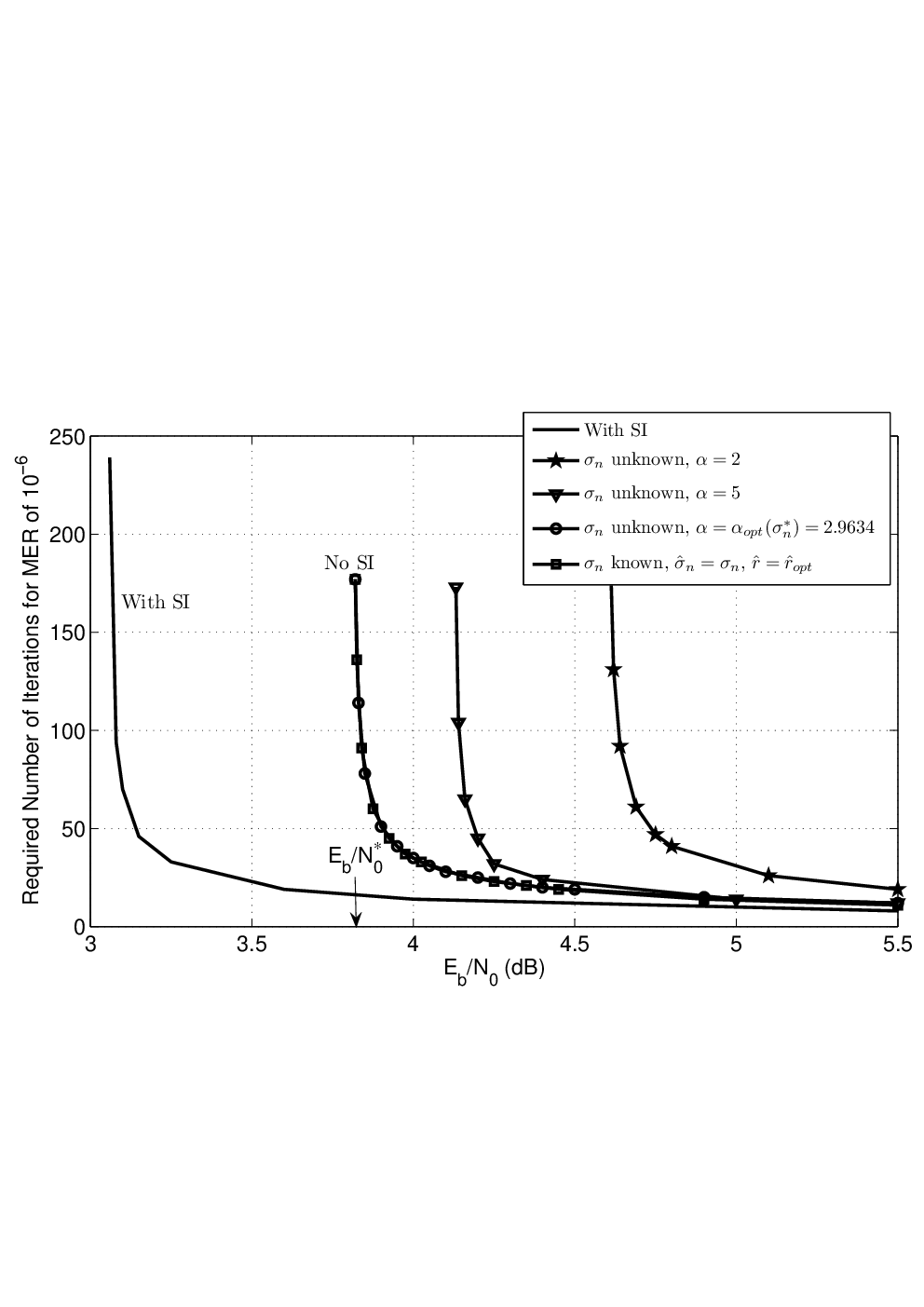
In order to measure the performance we do as follows. For various $\sigma_{n}$ and different values of $\alpha$ (including $\alpha_{\mathsf{opt}}(\sigma_{n})$), we find the required number of density evolution iterations to achieve a target message error-rate (MER) $p_{t}$ for a given LDPC code. We use the required number of iterations $\ell^{\ast}(p_{t})$ as a comparison measure and to identify the range of convergence.

In Fig. 4, different values of $\alpha$ are used and $\ell^{\ast}(p_{t})$ is plotted for different values of $\sigma_{n}$ for $\mathcal{C}^{\infty}(x^{2},x^{5})$. It is seen that by using $\alpha=\alpha_{\mathsf{opt}}(\sigma_{n}^{\ast}=0.6442)=2.9634$, the code has the widest convergence range. Interestingly, while this choice of $\alpha$ is not optimum for all values of $\sigma_{n}$, the resulted $\ell^{\ast}(p_{t})$ is always very close to the curve based on known $\sigma_{n}$ under MCLA. This observation can also be made from Fig. 3. The threshold of this code is at 3.06 dB with SI and is at 3.82 dB with no SI under MCLA. Thus, the gap between these thresholds is 0.76 dB. At this code rate, existence of SI results in about 0.74 dB improvement [8, 4]. Thus, MCLA shows a minor extra gap (0.02 dB) compared to true LLR calculation.

When $\sigma_{n}$ is unknown, one can design an LDPC code with a given rate which under MCLA provides the widest convergence region, i.e., has the largest decoding threshold. This procedure has to be done carefully, because $\alpha_{\mathsf{opt}}$ is a function of $\sigma_{n}^{\ast}$ which is initially unknown. We omit the details of this code design procedure in the interest of available space, but one designed code is reported in Table I (Code2). Again, 11-bit decoding under MCLA is used, the maximum number of iterations allowed is 300 and $d_{v}=30$. The threshold of the designed code is 2.76 dB. This code has the largest decoding threshold among all the codes with the rate 0.5.

We proposed a new method for linear LLR calculation on fading channels when channel fading gain is not known at the receiver. Our method is optimum in the sense of maximum achievable rate on the channel. We showed that on a Rayleigh channel, the maximum achievable rate using this method is extremely close to the channel capacity. Compared to existing work, which uses the expected value of the fading gain for LLR calculation, we reported considerable performance improvement at no extra decoding cost. This improvement would become more significant when the code rate increases.

We then extended our approach to the cases that the additive noise power of the fading channel is also unknown at the receiver. With a careful choice of linear LLR calculation, we were able to obtain a performance almost identical to the previous case, where the additive noise power was known.

For applications that channel estimation results in significant overheads or suffers from severe imperfections, our proposed solution can be of interest.

While we verified some of our results through study and design of LDPC codes on Rayleigh channel, our approach for maximizing the achievable transmission rate and convergence range of the decoder is general. The only reason for using LDPC codes is that, they can approach theoretical limits and thus verify some of our asymptotic results.

References

- [1] R. G. Gallager, “Low-Density Parity-Check codes,” Ph.D. dissertation, M.I.T press, Cambridge, MA, 1963.
- [2] C. Berrou, A. Glavieux, and P. Thitimajshima, “Near Shannon limit error-correcting coding and decoding: Turbo-codes (1),” in Conf. Rec. IEEE ICC ’93, vol. 2, Geneva, Switzerland, May 1993, pp. 1064–1070.
- [3] S.-Y. Chung, G. D. Forney, T. J. Richardson, and R. Urbanke, “On the design of low-density perity-check codes within 0.0045 dB of the Shannon limit,” IEEE Commun. Lett., vol. 5, no. 2, pp. 58–60, Feb. 2001.
- [4] J. Hou, P. H. Siegel, and L. B. Milstein, “Performance analysis and code optimization of low-density parity-check codes on Rayleigh fading channels,” IEEE J. Select. Areas Commun., vol. 19, no. 5, pp. 924–934, May 2001.
- [5] K. Fu and A. Anastasopoulos, “Performance analysis of LDPC codes for time-selective complex fading channels,” in GLOBECOM’02, vol. 2, Nov. 2002, pp. 1279–1283.
- [6] J. Lin and W. Wu, “Performance analysis of LDPC codes on Rician fading channels,” Higher Education Press and Springer-Verlag, 2006.
- [7] J. Xiaowei, A. W. Eckford, and T. E. Fuja, “Design of good low-density parity-check codes for block fading channels,” in MILCOM 2004, vol. 2, 2004, pp. 1054–1059.
- [8] E. K. Hall, “Performance and design of Turbo codes on Rayleigh fading channels,” Master’s thesis, University of Virginia, May 1996.
- [9] J. Hagenauer, “Viterbi decoding of convolutional codes for fading- and burst-channels,” in Zurich seminar on digital communications, 1980.
- [10] T. J. Richardson, M. A. Shokrollahi, and R. L. Urbanke, “Design of capacity-approaching irregular low-density parity-check codes,” IEEE Trans. Inform. Theory, vol. 47, no. 2, pp. 619–637, Feb. 2001.
- [11] O. Etesami and A. Shokrollahi, “Raptor codes on binary memoryless symmetric channels,” IEEE Trans. Inform. Theory, vol. 52, no. 5, pp. 2033–2051, 2006.
- [12] F. R. Kschischang, B. J. Frey, and H.-A. Loeliger, “Factor graphs and the sum-product algorithm,” IEEE Trans. Inform. Theory, vol. 47, pp. 498–519, Feb. 2001.
- [13] T. J. Richardson and R. L. Urbanke, “The capacity of low-density parity-check codes under message-passing decoding,” IEEE Trans. Inform. Theory, vol. 47, no. 2, pp. 599–618, Feb. 2001.