跳到论文正文
W Papers独立论文阅读器 arXiv:0704.2400 论文正文 计算阅读时间 · 0%
引用这篇论文根据当前论文元数据生成,正式投稿前建议核对。


License: Assumed arXiv.org perpetual non-exclusive license
arXiv:0704.2400v2 [hep-ph] 27 Apr 2007

DESY 07-053
SFB/CPP-07-15
HEPTOOLS 07-010

Two-Loop Fermionic Corrections
to Massive Bhabha Scattering

Stefano Actisa,  Michał Czakonb,c,  Janusz Gluzad,  Tord Riemanna

aDeutsches Elektronen-Synchrotron, DESY,
Platanenallee 6, D-15738 Zeuthen, Germany
bInstitut für Theoretische Physik und Astrophysik, Universität Würzburg,
Am Hubland, D-97074 Würzburg, Germany
cInstitute of Nuclear Physics, NCSR “DEMOKRITOS”,
15310 Athens, Greece
dInstitute of Physics, University of Silesia,
Uniwersytecka 4, PL-40007 Katowice, Poland

We evaluate the two-loop corrections to Bhabha scattering from fermion loops in the context of pure Quantum Electrodynamics. The differential cross section is expressed by a small number of Master Integrals with exact dependence on the fermion masses me,mfm_{e},m_{f} and the Mandelstam invariants s,t,us,t,u. We determine the limit of fixed scattering angle and high energy, assuming the hierarchy of scales me2≪mf2≪s,t,um_{e}^{2}\ll m_{f}^{2}\ll s,t,u. The numerical result is combined with the available non-fermionic contributions. As a by-product, we provide an independent check of the known electron-loop contributions.

1 Introduction

Bhabha scattering is one of the processes at e+​e−e^{+}e^{-} colliders with the highest experimental precision and represents an important monitoring process. A notable example is its expected role for the luminosity determination at the future International Linear Collider ILC by measuring small-angle Bhabha-scattering events at center-of-mass energies ranging from about 100 GeV (Giga-Z collider option) to several TeV. Moreover, the large-angle region is relevant at colliders operating at 1--10 GeV. For some applications a full two-loop calculation of the QED contributions is mandatory11 1 Note that leading two-loop effects in the electroweak Standard Model were already incorporated in [1]..

A large class of QED two-loop corrections was determined in the seminal work of [2]. Later, the complete two-loop corrections in the limit of zero electron mass were obtained in [3] thanks to the fundamental results of [4, 5]. However, this result cannot be immediately applied, since the available Monte-Carlo programs (see e.g. [6, 7, 8, 9, 10, 11, 12, 13]) employ a small, but non-vanishing electron mass. The α2​ln⁡(s/me2)\alpha^{2}\ln(s/m_{e}^{2}) terms due to double boxes were derived from [3] by the authors of [14], and the close-to-complete two-loop result in the ultra-relativistic limit was finally obtained in [15, 16]. Note that the diagrams with fermion loops have not been covered by this approach. The virtual and real components involving electron loops could be added exactly in [17, 18]. The non-approximated analytical expressions for all two-loop corrections, except for double-box diagrams and for those with loops from heavier-fermion generations, can be found in [19]. For a comprehensive investigation of the full set of the massive two-loop QED corrections, including double-box diagrams, we refer to [20, 21, 22]. The evaluation of the contributions from massive non-planar double box diagrams remains open so far.

In order to add another piece to the complete two-loop prediction for the Bhabha-scattering cross section in QED, we evaluate here the so-far lacking diagrams containing heavy-fermion loops. The cross section correction is expressed by a small number of scalar Master Integrals, where the exact dependence on the masses of the fermions and the Mandelstam variables ss, tt and uu is retained. In a next step, we assume a hierarchy of scales, me2≪mf2≪s,t,um_{e}^{2}\ll m_{f}^{2}\ll s,t,u, where mem_{e} is the electron mass and mfm_{f} is the mass of a heavier fermion. We derive explicit results neglecting terms suppressed by positive powers of me2/mf2m_{e}^{2}/\penalty m_{f}^{2}, me2/xm_{e}^{2}/\penalty x and mf2/xm_{f}^{2}/\penalty x, where x=s,t,ux=s,t,u. This high-energy approximation describes the influence of muons and τ\tau leptons and proves well-suited for practical applications. In addition, we provide an independent cross-check of the exact analytical results of [17] (we used the files provided at [23] for comparison) for mf=mem_{f}=m_{e}.

The article is organized as follows. In Section 2 we introduce our notations and outline the calculation and in Section 3 we discuss the solution for each class of diagrams. In Section 4 we reproduce the complete result for the corrections from heavier fermions in analytic form and perform the numerical analysis. Section 5 contains the summary, and additional material on the Master Integrals is collected in the Appendix.

2 Expansion of the Cross Section

We consider the Bhabha-scattering process,

e−(p1)+e+(p2)→e−(p3)+e+(p4),e^{{}_{-}}\,(p_{1})\,+\,e^{{}_{+}}\,(p_{2})\,\to\,e^{{}_{-}}\,(p_{3})\,+\,e^{{}_{+}}\,(p_{4}), (2.1)

and introduce the Mandelstam invariants ss, tt and uu,

s\displaystyle s =\displaystyle= (p1+p2)2=4​E2,\displaystyle\left(\,p_{1}+p_{2}\,\right)^{2}=4\,E^{2}, (2.2)
t\displaystyle t =\displaystyle= (p1−p3)2=−4​(E2−me2)​sin2⁡θ2,\displaystyle\left(\,p_{1}-p_{3}\,\right)^{2}=-4\left(\,E^{2}\,-\,m_{e}^{2}\,\right)\,\sin^{2}\frac{\theta}{2}, (2.3)
u\displaystyle u =\displaystyle= (p1−p4)2=−4​(E2−me2)​cos2⁡θ2,\displaystyle\left(\,p_{1}-p_{4}\,\right)^{2}=-4\left(\,E^{2}\,-\,m_{e}^{2}\,\right)\,\cos^{2}\frac{\theta}{2}, (2.4)

where mem_{e} is the electron mass, EE is the incoming-particle energy in the center-of-mass frame and θ\theta is the scattering angle. In addition, s+t+u= 4​me2.s\,+\,t\,+\,u\,=\,4\,m_{e}^{2}.

In the kinematical region me2≪s,t,um_{e}^{2}\ll s,t,u the leading-order (LO) differential cross section with respect to the solid angle Ω\Omega reads as

d​σLOd​Ω=α2s​[1s2​(s22+t2+s​t)+1t2​(t22+s2+s​t)+1s​t​(s+t)2],\frac{d\sigma^{\rm{{\scriptscriptstyle{L}}{\scriptscriptstyle{O}}}}}{d\Omega}\,=\,\frac{\alpha^{2}}{s}\,\Bigl[\,\frac{1}{s^{2}}\,\Bigl(\,\frac{s^{2}}{2}\,+\,t^{2}\,+\,s\,t\,\Bigr)\,+\,\frac{1}{t^{2}}\,\Bigl(\,\frac{t^{2}}{2}\,+\,s^{2}\,+\,s\,t\,\Bigr)\,+\,\frac{1}{s\,t}\,\left(\,s\,+\,t\,\right)^{2}\,\Bigr], (2.5)

where α\alpha is the fine-structure constant. At higher orders in perturbation theory we write an expansion in α\alpha,

d​σd​Ω=d​σLOd​Ω+(απ)​d​σNLOd​Ω+(απ)2​d​σNNLOd​Ω+𝒪⁡(α5).\frac{d\sigma}{d\Omega}\,=\,\frac{d\sigma^{\rm{{\scriptscriptstyle{L}}{\scriptscriptstyle{O}}}}}{d\Omega}\,+\,\left(\frac{\alpha}{\pi}\right)\frac{d\sigma^{\rm{{\scriptscriptstyle{N}}{\scriptscriptstyle{L}}{\scriptscriptstyle{O}}}}}{d\Omega}\,+\,\left(\frac{\alpha}{\pi}\right)^{2}\frac{d\sigma^{\rm{{\scriptscriptstyle{N}}{\scriptscriptstyle{N}}{\scriptscriptstyle{L}}{\scriptscriptstyle{O}}}}}{d\Omega}+{\cal O}(\alpha^{5}). (2.6)

Here d​σNLOd\sigma^{\rm{{\scriptscriptstyle{N}}{\scriptscriptstyle{L}}{\scriptscriptstyle{O}}}} and d​σNNLOd\sigma^{\rm{{\scriptscriptstyle{N}}{\scriptscriptstyle{N}}{\scriptscriptstyle{L}}{\scriptscriptstyle{O}}}} summarize the next-to-leading order (NLO) and next-to-next-to-leading order (NNLO) corrections to the differential cross section. In the following it will be understood that we consider only components generated by diagrams containing one or two fermion loops.

Refer to caption
Figure 1: Classes of Bhabha-scattering one-loop diagrams. A thin fermion line represents an electron, a thick one can be any fermion. The full set of graphs can be obtained through proper permutations. We refer to [24] for the reproduction of the full set of graphs.

2.1 NLO Differential Cross Section

The NLO term follows from the interference of the one-loop vacuum-polarization diagrams of class 1a (see Figure 1) with the tree-level amplitude,

d​σNLOd​Ω=d​σ1​a×treed​Ω=α2s\displaystyle\frac{d\sigma^{\rm{{\scriptscriptstyle{N}}{\scriptscriptstyle{L}}{\scriptscriptstyle{O}}}}}{d\Omega}\,=\,\frac{d\sigma^{\rm{1a}\times\rm{tree}}}{d\Omega}=\frac{\alpha^{2}}{s} {\displaystyle\Bigl\{ 1s2​(s22+t2+s​t)​  2​∑fQf2​Re​[Πf(1)​(s)]\displaystyle\frac{1}{s^{2}}\,\Bigl(\,\frac{s^{2}}{2}\,+\,t^{2}\,+\,s\,t\,\Bigr)\,\,2\,\sum_{f}\,Q_{f}^{2}\,\text{Re}\,\Bigl[\,\Pi^{(1)}_{f}(s)\,\Bigr] (2.7)
+\displaystyle+ 1t2​(t22+s2+s​t)​  2​∑fQf2​Re​[Πf(1)​(t)]\displaystyle\frac{1}{t^{2}}\,\Bigl(\,\frac{t^{2}}{2}\,+\,s^{2}\,+\,s\,t\,\Bigr)\,\,2\,\sum_{f}\,Q_{f}^{2}\ \text{Re}\,\Bigl[\,\Pi^{(1)}_{f}(t)\,\Bigr]
+\displaystyle+ 1s​t(s+t)2∑fQf2Re[Πf(1)(s)+Πf(1)(t)]}.\displaystyle\frac{1}{s\,t}\,\left(\,s\,+\,t\,\right)^{2}\,\,\sum_{f}\,Q_{f}^{2}\,\text{Re}\,\Bigl[\,\Pi^{(1)}_{f}(s)\,+\,\Pi^{(1)}_{f}(t)\,\Bigr]\,\,\,\Bigr\}.

Here Πf(1)​(x)\Pi^{(1)}_{f}(x) is the renormalized one-loop vacuum-polarization function and the sum over ff runs over the massive fermions, e.g. the electron (f=ef=e), the muon (f=μf=\mu), the τ\tau lepton (f=τf=\tau). QfQ_{f} is the electric-charge quantum number, Qf=−1Q_{f}=-1 for leptons.

In this paper we will focus on asymptotic expansions in the high-energy limit. In order to fix our normalizations explicitly, we reproduce here the exact result for Πf(1)​(x)\Pi^{(1)}_{f}(x) in dimensional regularization. Adding Πf(1)​c​t​(x)\Pi^{(1)ct}_{f}(x), the counterterm contribution in the on-mass-shell scheme (see the following discussion in Subsection 2.3), to Πf(1)​u​n​(x)\Pi^{(1)un}_{f}(x), the unrenormalized one-loop vacuum polarization function, we get

Πf(1)​(x)\displaystyle\Pi^{(1)}_{f}(x) =\displaystyle= Πf(1)​u​n​(x)+Πf(1)​c​t​(x),\displaystyle\Pi^{(1)un}_{f}(x)+\Pi^{(1)ct}_{f}(x), (2.8)
Πf(1)​u​n​(x)\displaystyle\Pi^{(1)un}_{f}(x) =\displaystyle= 12​(D−1)​[2​(D−2)​1x​A0​(mf)−(D−2+4​mf2x)​B0​(x,mf)],\displaystyle\frac{1}{2(D-1)}\left[2(D-2)\frac{1}{x}A_{0}(m_{f})-\left(D-2+4\frac{m_{f}^{2}}{x}\right)B_{0}(x,m_{f})\right], (2.9)
Πf(1)​c​t​(x)\displaystyle\Pi^{(1)ct}_{f}(x) =\displaystyle= 13​Fϵ​(me2mf2)ϵ​(1ϵ+ζ22​ϵ),\displaystyle\frac{1}{3}F_{\epsilon}\left(\frac{m_{e}^{2}}{m_{f}^{2}}\right)^{\epsilon}\left(\frac{1}{\epsilon}+\frac{\zeta_{2}}{2}\epsilon\right), (2.10)

where ϵ=(4−D)/2\epsilon=(4-D)/\penalty 2 and DD is the number of space-time dimensions. The normalization factor is

Fϵ=(me2​π​eγEμ2)−ϵ,F_{\epsilon}\,=\,\,\left(\,\frac{m_{e}^{2}\,\pi\,e^{\gamma_{E}}}{\mu^{2}}\,\right)^{-\epsilon}, (2.11)

μ\mu is the ’t Hooft mass unit and γE\gamma_{E} is the Euler-Mascheroni constant. Standard one-loop integrals appearing in Eq. (2.8) are defined by

A0​(m)\displaystyle A_{0}(m) =\displaystyle= μ4−Di​π2​∫dD​k​1k2−m2,\displaystyle\frac{\mu^{4-D}}{i\pi^{2}}\int d^{D}k\frac{1}{k^{2}-m^{2}}, (2.12)
B0​(p2,m)\displaystyle B_{0}(p^{2},m) =\displaystyle= μ4−Di​π2​∫dD​k​1(k2−m2)​[(k+p)2−m2].\displaystyle\frac{\mu^{4-D}}{i\pi^{2}}\int d^{D}k\frac{1}{(k^{2}-m^{2})[(k+p)^{2}-m^{2}]}. (2.13)

Note that Master Integrals with l lines and an internal scale mm were derived in [20, 24] setting m=1m=1. For the present computation we introduce a scaling by a factor mfD−2​lm_{f}^{D-2l} and we get

A0​(mf)\displaystyle A_{0}(m_{f}) =\displaystyle= Fϵ​(me2mf2)ϵ​mf2​T1l1m,\displaystyle F_{\epsilon}\,\left(\frac{m_{e}^{2}}{m_{f}^{2}}\right)^{\epsilon}~\,m_{f}^{2}~\,\texttt{T1l1m}, (2.14)
B0​(x,mf)\displaystyle B_{0}(x,m_{f}) =\displaystyle= Fϵ​(me2mf2)ϵ​SE2l2m[x].\displaystyle F_{\epsilon}\,\left(\frac{m_{e}^{2}}{m_{f}^{2}}\right)^{\epsilon}\texttt{SE2l2m[x]}. (2.15)

In the small-mass limit, A0A_{0} vanishes (the result for T1l1m can be read in Eq.(4) of [20]), and the one-loop self-energy22 2 Here, the argument xx of SE2l2m[x] is one of the relativistic invariants s,t,us,t,u. This deviates from earlier conventions, where we denoted by xx the dimensionless conformal transform of s,t,us,t,u. This remark applies also to Master Integrals in the Appendix. reads as

SE2l2m[x]=1ϵ+2+Lf​(x)+ϵ⁡[4−ζ22+2​Lf​(x)+12​Lf2​(x)],\texttt{SE2l2m[x]}=\frac{1}{\epsilon}+2+L_{f}(x)+\epsilon\left[4-\frac{\zeta_{2}}{2}+2\,L_{f}(x)+\frac{1}{2}\,L^{2}_{f}(x)\right]\,, (2.16)

where we introduced the short-hand notation for logarithmic functions (in our conventions the logarithm has a cut along the negative real axis),

Lf​(x)=ln⁡(−mf2x+i​δ),δ→0+.L_{f}(x)\,=\,\ln\left(\,-\,\frac{m_{f}^{2}}{x+\,i\,\delta}\,\right),\qquad\delta\to 0_{+}. (2.17)

Finally, neglecting 𝒪⁡(mf2/x){\cal O}(m_{f}^{2}/x) terms, Πf(1)​(x)\Pi^{(1)}_{f}(x) reads as

Πf(1)​(x)=−Fϵ3​(me2mf2)ϵ​{53+Lf​(x)+ϵ⁡[289−ζ2+53​Lf​(x)+12​Lf2​(x)]}.\Pi^{(1)}_{f}(x)\,=\,-\,\frac{F_{\epsilon}}{3}\,\left(\frac{m_{e}^{2}}{m_{f}^{2}}\right)^{\epsilon}\,\left\{\,\frac{5}{3}\,+\,L_{f}(x)\,+\,\epsilon\,\left[\,\frac{28}{9}\,-\,\zeta_{2}\,+\,\frac{5}{3}\,L_{f}(x)\,+\,\frac{1}{2}\,L_{f}^{2}(x)\,\,\right]\,\right\}. (2.18)

Note that the 𝒪⁡(ϵ){\cal O}(\epsilon) term in Eq. (2.18) is not required for the NLO computation, but it will become relevant at NNLO. Here Πf(1)​(x)\Pi^{(1)}_{f}(x) will be combined with infrared-divergent graphs showing single poles in the ϵ\epsilon plane for ϵ=0\epsilon=0. The exact result for Πf(1)​(x)\Pi^{(1)}_{f}(x) is available at [24].

Refer to caption
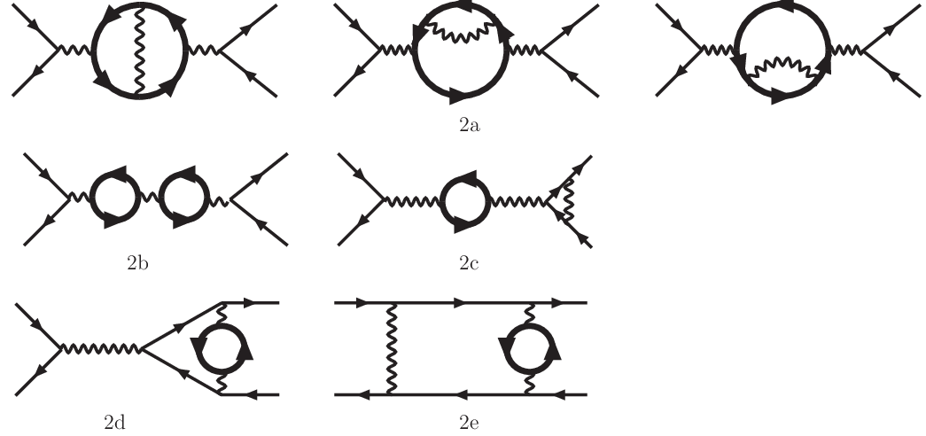
Figure 2: Classes of Bhabha-scattering two-loop diagrams containing at least one fermion loop. We use the conventions of Figure 1. Note that class 2a contains three topologically different subclasses. We refer to [24] for the reproduction of the full set of graphs.

2.2 Outline of the NNLO Computation

At NNLO we have to consider:

  • •

    The interference of the two-loop diagrams of classes 2a-2e (see Figure 2) with the tree-level amplitude;

  • •

    The interference of the one-loop vacuum-polarization diagrams of class 1a with the full set of graphs of classes 1a-1c (see Figure 1).

The complete result can be organized as

d​σNNLOd​Ω=∑i=a,…,ed​σ2​i×treed​Ω⏟2−loop×tree+∑i=a,…,cd​σ1​a×1​id​Ω⏟1−loop×1−loop.\frac{d\sigma^{\rm{{\scriptscriptstyle{N}}{\scriptscriptstyle{N}}{\scriptscriptstyle{L}}{\scriptscriptstyle{O}}}}}{d\Omega}\,=\,\underbrace{\sum_{\rm{i}=\rm{a},\ldots,\rm{e}}\frac{d\sigma^{\rm{2i}\times\rm{tree}}}{d\Omega}}_{\rm{2-loop}\times\rm{tree}}\,+\,\underbrace{\sum_{\rm{i}=\rm{a},\ldots,\rm{c}}\frac{d\sigma^{\rm{1a}\times\rm{1i}}}{d\Omega}}_{\rm{1-loop}\times\rm{1-loop}}. (2.19)
Refer to caption
Figure 3: Counterterm-dependent Feynman rules relevant for Bhabha scattering for i=1i=1 (one loop) and i=2i=2 (two loops). Note that in the on-mass-shell scheme e2=4​π​αe^{2}=4\pi\alpha at all orders in perturbation theory.

In order to compute the NNLO differential cross section we use the following reduction strategy:

  • •

    The generation of all the diagrams is simple and has been made with the computer-algebra systems GraphShot [25] and qgraf/DIANA [26, 27, 28]. We spin-sum the squared matrix elements and take the traces over Dirac indices in DD dimensions using the computer-algebra system FORM [29]. The resulting expressions are combinations of algebraic coefficients depending on s,t,u,me,mfs,t,u,m_{e},m_{f} and ϵ\epsilon and two-loop integrals with scalar products containing the loop momenta in the numerators. An example showing the complexity of the result (two-loop box diagram of class 2e, see Figure 2) can be found at [24].

  • •

    We reduce the loop integrals to a set of Master Integrals by means of the IdSolver implementation [30] of the Laporta algorithm [31, 32]. The complete list of massive Bhabha-scattering Master Integrals can be found in [20].

Next, we evaluate the Master Integrals:

  • •

    Integrals arising from graphs of classes 1a-1c (Figure 1), 2a-2c (Figure 2) and 2d-2e (Figure 2, with electron loops) have been computed exactly through the method of differential equations in the external kinematic variables and expressed through Harmonic Polylogarithms [33] or Generalized Harmonic Polylogarithms [34, 35]. Here we agree perfectly with the work of [17, 23]. Non-approximated results for the various components of the differential cross section are collected in a  Mathematica [36] file at [24].

  • •

    Integrals generated by the diagrams of classes 2d-2e (Figure 2, with heavy-fermion loops) are computed through a method based on asymptotic expansions of Mellin-Barnes representations. We derived appropriate Mellin-Barnes representations [37, 38] for each Master Integral and performed an analytic continuation in ϵ\epsilon from a range where the integral is regular to the origin of the ϵ\epsilon plane [4, 5]. This is done by an automatic procedure implemented in the package MB.m [39]. To proceed further, we assume a hierarchy of scales, me2≪mf2≪s,t,um_{e}^{2}\ll m_{f}^{2}\ll s,t,u, where f≠ef\neq e. After identifying the leading contributions in the fermion masses (in the same spirit as in [40]), we express the integrals by series over residua, and the latter are sumed up analytically in terms of polylogs by means of the package XSUMMER[41]. Asymptotic expansions for the master integrals with two different masses were given in [42]. They, and also few lacking expansions of simpler masters needed here have been collected in Appendix A. We refer for a detailed discussion to [22], where the technique was employed to derive approximated results for the massive Bhabha-scattering planar box master integrals. All the mass-expanded masters may also be found in a Mathematica file at [24].

2.3 Renormalization

In the following we will always deal with ultraviolet-renormalized quantities. After regularizing the theory using dimensional regularization [43, 44], we perform renormalization in the on-mass-shell scheme. Here we relate all free parameters to physical observables:

  • –

    The electric charge coincides with the value of the electromagnetic coupling, as measured in Thomson scattering, at all orders in perturbation theory;

  • –

    The squared fermion masses are identified with the real parts of the poles of the Dyson-resummed propagators;

  • –

    Finally, field-renormalization constants are chosen in order to cancel external wave-function corrections.

Counterterm-dependent Feynman rules are shown in Figure 3. Note that the presence of infrared divergencies at NNLO requires to compute one-loop counterterms including 𝒪⁡(ϵ){\cal O}(\epsilon) terms.

One-Loop Counterterms

The one-loop counterterms read as

δ​Zγ​γ1\displaystyle\delta Z^{1}_{\gamma\gamma} =\displaystyle= −Fϵ12​π2∑fQf2(me2mf2)ϵ(1ϵ+ϵ2ζ2),\displaystyle-\,\frac{F_{\epsilon}}{12\,\pi^{2}}\,\sum_{f}\,Q_{f}^{2}\,\Bigl(\frac{m_{e}^{2}}{m_{f}^{2}}\Bigr)^{\epsilon}\Bigl(\,\frac{1}{\epsilon}\,+\,\frac{\epsilon}{2}\,\zeta_{2}\,\Bigr), (2.20)
δ​Zf​f1\displaystyle\delta Z^{1}_{ff} =\displaystyle= δ​Zm1=−Fϵ16​π2​Qf2​(me2mf2)ϵ​[3ϵ+ 4+ϵ⁡( 8+32​ζ2)],\displaystyle\delta Z^{1}_{m}=-\,\frac{F_{\epsilon}}{16\,\pi^{2}}\,Q_{f}^{2}\,\Bigl(\frac{m_{e}^{2}}{m_{f}^{2}}\Bigr)^{\epsilon}\,\left[\,\frac{3}{\epsilon}\,+\,4\,+\,\epsilon\,\left(\,8\,+\,\frac{3}{2}\,\zeta_{2}\,\right)\,\right], (2.21)
δ​Zγ​f​f1\displaystyle\delta Z^{1}_{\gamma ff} =\displaystyle= δ​Zf​f1,\displaystyle\delta Z^{1}_{ff}, (2.22)

where the last equation follows from the U(1) QED Ward identity. In the ultrarelativistic limit, the one-loop fermion-mass counterterm is not needed, since it is always multiplied by the fermion mass. Note however that the same counterterm is relevant for the exact computation.

Two-Loop Counterterms

At the two-loop level we get

δ​Zγ​γ2\displaystyle\delta Z_{\gamma\gamma}^{2} =\displaystyle= −Fϵ2128​π4∑fQf4(me2mf2)2​ϵ(1ϵ+152),\displaystyle\,-\frac{F_{\epsilon}^{2}}{128\,\pi^{4}}\,\sum_{f}\,Q_{f}^{4}\,\Bigl(\frac{m_{e}^{2}}{m_{f}^{2}}\Bigr)^{2\epsilon}\Bigl(\,\frac{1}{\epsilon}\,+\,\frac{15}{2}\,\Bigr), (2.23)
δ​Zγ​e​e2\displaystyle\delta Z^{2}_{\gamma ee}\, =\displaystyle= Fϵ2128​π4​[12​ϵ+94736− 16​ζ2+∑f≠eQf2​(me2mf2)2​ϵ​(12​ϵ−512)].\displaystyle\,\frac{F_{\epsilon}^{2}}{128\,\pi^{4}}\,\Bigl[\,\frac{1}{2\,\epsilon}\,+\,\frac{947}{36}\,-\,16\,\zeta_{2}\,+\,\sum_{f\neq e}Q_{f}^{2}\Bigl(\frac{m_{e}^{2}}{m_{f}^{2}}\Bigr)^{2\epsilon}\Bigl(\,\frac{1}{2\,\epsilon}\,-\,\frac{5}{12}\,\,\Bigr)\Bigr]. (2.24)

The result for δ​Zγ​e​e2\delta Z^{2}_{\gamma ee} is obtained including just fermion-loop diagrams and neglecting 𝒪⁡(me2/mf2){\cal O}(m_{e}^{2}/\penalty m_{f}^{2}) terms for f≠ef\neq e. The expression for δ​Zγ​γ2\delta Z_{\gamma\gamma}^{2} (as well as the one-loop counterterms of Eqs. (2.20)-(2.22)), instead, is exact, since it follows from the single-scale diagrams of classes 2a-2b of Figure 2. Finally, we observe that the two-loop counterterm with two fermion lines is not required, since the use of an on-mass-shell renormalization removes external wave-function factors.

3 Two-Loop Corrections

In this Section we show our approximated results for all the components of the NNLO differential cross section of Eq. (2.6). Our short-hand notation for logarithmic functions can be found in Eq. (2.17). In addition, we define two combinations of the Mandelstam invariants:

v1​(x,y,ϵ)\displaystyle v_{1}(x,y;\epsilon)\, =\displaystyle= x2+ 2​y2+ 2​x​y−ϵ​x2,\displaystyle\,x^{2}\,+\,2\,y^{2}\,+\,2\,x\,y\,-\epsilon\,x^{2}, (3.1)
v2​(x,y,ϵ)\displaystyle v_{2}(x,y;\epsilon)\, =\displaystyle= (x+y)2−ϵ⁡(x2+y2+x​y),\displaystyle\,(\,x\,+\,y\,)^{2}\,-\,\epsilon\,(\,x^{2}\,+\,y^{2}\,+x\,y\,), (3.2)

where x⁡(y)=s,t,ux(y)=s,t,u. Note that for ϵ=0\epsilon=0 these functions are proportional to the kinematical factors appearing in the Born cross section of Eq. (2.5) and the NLO corrections of Eq. (2.7). Moreover, we introduce a compact notation which will prove useful in discussing box corrections in Subsection 3.3 and the complete NNLO differential cross section in Section 4,

L⁡(Rf)=ln⁡(me2mf2).L(R_{f})\,=\,\ln\,\left(\frac{m_{e}^{2}}{m_{f}^{2}}\right). (3.3)

3.1 Vacuum-Polarization Corrections

The interference of the vacuum-polarization diagrams of classes 2a and 2b with the tree-level amplitude can be written as

d​σ2​i×treed​Ω=α2s\displaystyle\frac{d\sigma^{\rm{2i}\times\rm{tree}}}{d\Omega}\,=\,\frac{\alpha^{2}}{s} {\displaystyle\Bigl\{ 1s2​v1​(s,t,0)​A2​i​(s)+1t2​v1​(t,s,0)​A2​i​(t)\displaystyle\frac{1}{s^{2}}\,\,v_{1}(s,t;0)\,\,A^{\rm{2i}}(s)\,\,+\,\frac{1}{t^{2}}\,\,v_{1}(t,s;0)\,\,A^{\rm{2i}}(t) (3.4)
+\displaystyle+ 1s​tv2(s,t;0)[A2​i(s)+A2​i(t)]},i=a,b.\displaystyle\frac{1}{s\,t}\,\,v_{2}(s,t;0)\,\,\Bigl[\,A^{\rm{2i}}(s)\,+\,A^{\rm{2i}}(t)\,\Bigr]\,\,\,\Bigr\},\qquad\rm{i}=\rm{a},\rm{b}.

Here we introduced the auxiliary functions A2​a​(x)A^{\rm{2a}}(x) and A2​b​(x)A^{\rm{2b}}(x), which are expressed through the renormalized one- and two-loop vacuum-polarization functions Πf(1)​(x)\Pi^{(1)}_{f}(x) (see Eq. (2.18) ) and Πf(2)​(x)\Pi^{(2)}_{f}(x),

A2​a​(x)\displaystyle A^{\rm{2a}}(x) =\displaystyle= ∑fQf4​Re​[Πf(2)​(x)],\displaystyle\sum_{f}\,Q_{f}^{4}\,\text{Re}\,\Bigl[\,\Pi^{(2)}_{f}(x)\,\Bigr], (3.5)
A2​b​(x)\displaystyle A^{\rm{2b}}(x) =\displaystyle= ∑f1,f2Qf12​Qf22​Re​[Πf1(1)​(x)​Πf2(1)​(x)],\displaystyle\sum_{f_{1},f_{2}}\,Q_{f_{1}}^{2}\,Q_{f_{2}}^{2}\,\text{Re}\,\Bigl[\,\Pi^{(1)}_{f_{1}}(x)\,\,\Pi^{(1)}_{f_{2}}(x)\,\Bigr], (3.6)

where the result for Πf(2)​(x)\Pi^{(2)}_{f}(x) in the small fermion-mass limit reads as

Πf(2)​(x)=−524+ζ3−14​Lf​(x).\Pi^{(2)}_{f}(x)\,=\,-\,\frac{5}{24}\,+\,\zeta_{3}-\,\frac{1}{4}\,L_{f}(x)\,. (3.7)

Note that 𝒪⁡(ϵ){\cal O}(\epsilon) terms in Eq. (3.4) coming from the kinematical coefficients of Eq. (3.1) can be safely neglected, since both Πf(1)​(x)\Pi^{(1)}_{f}(x) and Πf(2)​(x)\Pi^{(2)}_{f}(x) are infrared-finite quantities.

3.2 Vertex Corrections

The contribution of reducible (irreducible) vertex corrections to the NNLO differential cross section can be readily derived from diagrams of classes 2c (2d) in Figure 2,

d​σ2​i×treed​Ω= 2​α2s\displaystyle\frac{d\sigma^{\rm{2i}\times\rm{tree}}}{d\Omega}\,=\,2\,\frac{\alpha^{2}}{s} {\displaystyle\Bigl\{ 1s2​[v1​(s,t,ϵ)​AV2​i​(s)+s2​AM2​i​(s)]+1t2​[v1​(t,s,ϵ)​AV2​i​(t)+t2​AM2​i​(t)]\displaystyle\frac{1}{s^{2}}\,\Bigl[\,v_{1}(s,t;\epsilon)\,A_{\rm{V}}^{\rm{2i}}(s)\,\,+\,s^{2}\,A_{\rm{M}}^{\rm{2i}}(s)\Bigr]+\frac{1}{t^{2}}\,\Bigl[\,v_{1}(t,s;\epsilon)\,A_{\rm{V}}^{\rm{2i}}(t)\,\,+\,t^{2}\,A_{\rm{M}}^{\rm{2i}}(t)\,\Bigr] (3.8)
+\displaystyle+ 1s​t[v2(s,t;ϵ)(AV2​i(s)+AV2​i(t))+32(s2AM2​i(s)+t2AM2​i(t))\displaystyle\frac{1}{s\,t}\,\Bigl[\,v_{2}(s,t;\epsilon)\,\Bigl(\,A_{\rm{V}}^{\rm{2i}}(s)\,+\,A_{\rm{V}}^{\rm{2i}}(t)\,\Bigr)\,+\,\frac{3}{2}\,\Bigl(\,s^{2}\,A_{\rm{M}}^{\rm{2i}}(s)\,+\,t^{2}\,A_{\rm{M}}^{\rm{2i}}(t)\,\Bigr)\,
+\displaystyle+ 2st(AM2​i(s)+AM2​i(t))]},i=c,d.\displaystyle 2\,s\,t\,\Bigl(\,A_{\rm{M}}^{\rm{2i}}(s)\,+\,A_{\rm{M}}^{\rm{2i}}(t)\,\Bigr)\,\Bigr]\,\Bigr\},\qquad\rm{i}=\rm{c},\rm{d}.

Reducible diagrams

The auxiliary functions AV2​c​(x)A_{\rm{V}}^{\rm{2c}}(x) and AM2​c​(x)A_{\rm{M}}^{\rm{2c}}(x) are given by the product of the renormalized one-loop vacuum-polarization function Πf(1)​(x)\Pi^{(1)}_{f}(x) (expanded in Eq. (2.18) including 𝒪⁡(ϵ){\cal O}(\epsilon) terms) and the renormalized one-loop vector and magnetic vertex form factors FV(1)​(x)F^{(1)}_{\rm{V}}(x) and FM(1)​(x)F^{(1)}_{\rm{M}}(x),

AI2​c(x)=∑fQf2Re[FI(1)(x)Πf(1)(x)],I=V,M.A_{\rm{I}}^{\rm{2c}}(x)\,=\,\sum_{f}\,Q_{f}^{2}\,\text{Re}\,\Bigl[\,F^{(1)}_{\rm{I}}(x)\,\Pi^{(1)}_{f}(x)\,\Bigr],\qquad\rm{I}\,=\rm{V,M}. (3.9)

The asymptotic expansion of FV(1)​(x)F^{(1)}_{\rm{V}}(x) is given by

FV1​(x)=−Fϵ2​ϵ​[1+Le​(x)]− 1+12​ζ2−34​Le​(x)−14​Le2​(x),\begin{split}F^{1}_{\rm{V}}(x)\,&=\,-\,\frac{F_{\epsilon}}{2\epsilon}\,\,\Bigl[1\,+\,L_{e}(x)\Bigr]-\,1\,+\,\frac{1}{2}\,\zeta_{2}-\,\frac{3}{4}\,L_{e}(x)\,-\,\frac{1}{4}\,L_{e}^{2}(x)\,,\end{split} (3.10)

whereas FM(1)​(x)F^{(1)}_{\rm{M}}(x) vanishes when we neglect the electron mass, FM(1)​(x)= 0F^{(1)}_{\rm{M}}(x)\,=\,0. The renormalized one-loop vertex develops an infrared divergency, which shows up as a single pole in the ϵ\epsilon plane for ϵ=0\epsilon=0. Therefore, when computing the cross section, we sum over the spins the squared matrix element and we evaluate the traces over Dirac indices in D=4− 2​ϵD=4\,-\,2\,\epsilon dimensions. The needed kinematical structures include 𝒪⁡(ϵ){\cal O}(\epsilon) terms (see Eq. (3.1)).

Irreducible Diagrams

The renormalized two-loop vertex diagrams of class 2d are free of infrared divergencies. Therefore, we can neglect 𝒪⁡(ϵ){\cal O}(\epsilon) terms in the kinematical coefficients of Eq. (3.1) appearing in Eq. (3.8), setting va(x,y,;ϵ)=va(x,y;0)v_{a}(x,y,;\epsilon)=v_{a}(x,y;0), for a=1,2a=1,2. The auxiliary functions AV2​d​(x)A_{\rm{V}}^{\rm{2d}}(x) and AM2​d​(x)A_{\rm{M}}^{\rm{2d}}(x) contain the renormalized two-loop vector and magnetic vertex form factors (see [45, 46, 47] for a detailed discussion),

AI2​d(x)=∑fQf2Re[FI,f(2)(x)],I=V,M.A_{\rm{I}}^{\rm{2d}}(x)\,=\,\sum_{f}\,Q_{f}^{2}\,\text{Re}\,\Bigl[\,F^{(2)}_{{\rm{I}},f}(x)\,\Bigr],\qquad\rm{I}\,=\rm{V,M}. (3.11)

For the case with an electron loop, FI,e(2)​(x)F^{(2)}_{\rm{I},e}(x), the exact results in terms of Harmonic Polylogarithms, can be readily expanded in the high-energy limit. For the vector term we get

FV,e(2)​(x)=14​(38327−ζ2)+16​(26536+ζ2)​Le​(x)+1972​Le2​(x)+136​Le3​(x).\begin{split}F^{(2)}_{{\rm{V}},e}(x)\,&=\,\frac{1}{4}\,\Bigl(\,\frac{383}{27}\,-\,\zeta_{2}\,\Bigr)\,+\,\frac{1}{6}\left(\,\frac{265}{36}\,+\,\zeta_{2}\,\right)\,L_{e}(x)\,+\,\frac{19}{72}\,L_{e}^{2}(x)\,+\,\frac{1}{36}\,L_{e}^{3}(x).\end{split} (3.12)

For FV,f(2)​(x)F^{(2)}_{\rm{V},f}(x), f≠ef\neq e, we perform an asymptotic expansion of the Master Integrals arising in the computation (see Table V in [20]) and we fully agree with the result of [48],

FV,f(2)​(x)=16​(3355216+196​ζ2− 2​ζ3)+16​(26536+ζ2)​Lf​(x)+1972​Lf2​(x)+136​Lf3​(x).\begin{split}F^{(2)}_{{\rm{V}},f}(x)\,&=\,\frac{1}{6}\,\Bigl(\,\frac{3355}{216}\,+\,\frac{19}{6}\,\zeta_{2}\,-\,2\,\zeta_{3}\,\Bigr)\,+\,\frac{1}{6}\left(\,\frac{265}{36}\,+\,\zeta_{2}\,\right)\,L_{f}(x)\,+\,\frac{19}{72}\,L_{f}^{2}(x)\,+\,\frac{1}{36}\,L_{f}^{3}(x).\end{split} (3.13)

Since collinear logarithms are absent, the logarithmic structure of Eqs. (3.12) and (3.13) is obviously the same.

3.3 Box Corrections

The contribution of the renormalized two-loop box diagrams of class 2e is given by

d​σ2​e×treed​Ω=α22​s​[1s​A12​e×tree​(s,t)+1t​A22​e×tree​(s,t)].\begin{split}\frac{d\sigma^{\rm{2e}\times\rm{tree}}}{d\Omega}\,=\,\frac{\alpha^{2}}{2\,s}\,\Bigl[\,\frac{1}{s}\,A_{1}^{\rm{2e}\times\rm{tree}}(s,t)\,+\,\frac{1}{t}\,A_{2}^{\rm{2e}\times\rm{tree}}(s,t)\,\Bigr].\end{split} (3.14)

Here the auxiliary functions can be conveniently expressed through three independent form factors BI,f(2)​(x,y)B^{(2)}_{\rm{I},f}(x,y), where i=A,B,C\rm{i}=\rm{A},\rm{B},\rm{C},

A12​e×tree​(s,t)\displaystyle A_{1}^{\rm{2e}\times\rm{tree}}(s,t)\, =\displaystyle= Fϵ2​∑fQf2​Re​[BA,f(2)​(s,t)+BB,f(2)​(t,s)+BC,f(2)​(u,t)−BB,f(2)​(u,s)],\displaystyle\,F_{\epsilon}^{2}\sum_{f}\,Q_{f}^{2}\,\text{Re}\,\Bigl[\,B^{(2)}_{{\rm{A}},f}(s,t)\,+\,B^{(2)}_{{\rm{B}},f}(t,s)\,+\,B^{(2)}_{{\rm{C}},f}(u,t)\,-\,B^{(2)}_{{\rm{B}},f}(u,s)\,\Bigr], (3.15)
A22​e×tree​(s,t)\displaystyle A_{2}^{\rm{2e}\times\rm{tree}}(s,t)\, =\displaystyle= Fϵ2​∑fQf2​Re​[BB,f(2)​(s,t)+BA,f(2)​(t,s)−BB,f(2)​(u,t)+BC,f(2)​(u,s)].\displaystyle\,F_{\epsilon}^{2}\sum_{f}\,Q_{f}^{2}\,\text{Re}\,\Bigl[\,B^{(2)}_{{\rm{B}},f}(s,t)\,+\,B^{(2)}_{{\rm{A}},f}(t,s)\,-\,B^{(2)}_{{\rm{B}},f}(u,t)\,+\,B^{(2)}_{{\rm{C}},f}(u,s)\,\Bigr]. (3.16)

Electron Loops

For the case with an electron loop, BI,e(2)​(x,y)B^{(2)}_{\rm{I},e}(x,y), we get exact results in terms of Harmonic Polylogarithms and Generalized Harmonic Polylogarithms. An asymptotic expansion in the limit me2≪s,t,um_{e}^{2}\ll s,t,u leads to

BA,e(2)​(x,y)\displaystyle B_{{\rm{A}},e}^{(2)}(x,y) =\displaystyle= 1ϵ23(x2y+ 2x+y)[53+Le(y)]Le(x)+13x2y{−23(173+ 20ζ2)\displaystyle\frac{1}{\epsilon}\,\frac{2}{3}\,\Bigl(\,\frac{x^{2}}{y}\,+\,2\,x\,+\,y\,\Bigr)\,\Bigl[\,\frac{5}{3}\,+\,L_{e}(y)\,\Bigr]\,L_{e}(x)+\frac{1}{3}\,\frac{x^{2}}{y}\,\Bigl\{\,-\,\frac{2}{3}\,\Bigl(\,\frac{17}{3}\,+\,20\,\zeta_{2}\,\Bigr)\, (3.17)
+\displaystyle+ 2​(419−ζ2)​Le​(x)− 2​(13+ 8​ζ2)​Le​(y)−236​Le2​(y)+ 8​Le​(x)​Le​(y)\displaystyle 2\,\Bigl(\,\frac{41}{9}\,-\,\zeta_{2}\,\Bigr)\,L_{e}(x)\,-\,2\,\Bigl(\,\frac{1}{3}\,+\,8\,\zeta_{2}\,\Bigr)\,L_{e}(y)-\frac{23}{6}\,L^{2}_{e}(y)\,+\,8\,L_{e}(x)\,L_{e}(y)
−\displaystyle- 53​Le3​(y)+ 4​Le​(x)​Le2​(y)−[ 6​ζ2+ln2⁡(yx)]​ln⁡(1+yx)−2​ln⁡(yx)​Li2​(−yx)\displaystyle\frac{5}{3}\,L^{3}_{e}(y)+\,4\,L_{e}(x)\,L^{2}_{e}(y)-\Bigl[\,6\,\zeta_{2}\,+\,\ln^{2}\left(\frac{y}{x}\right)\,\Bigr]\,\ln\left(1+\frac{y}{x}\right)-2\,\ln\left(\frac{y}{x}\right)\,\text{Li}_{\rm{2}}\left(-\frac{y}{x}\right)
+\displaystyle+ 2Li3(−yx)}+x3{−23(343+ 7ζ2)+2429Le(x)− 4(53+ 6ζ2)Le(y)\displaystyle 2\,\text{Li}_{\rm{3}}\left(-\frac{y}{x}\right)\,\Bigr\}+\frac{x}{3}\,\Bigl\{\,-\,\frac{2}{3}\,\Bigl(\,\frac{34}{3}\,+\,7\,\zeta_{2}\,\Bigr)\,+\,\frac{242}{9}\,L_{e}(x)\,-\,4\,\Bigl(\,\frac{5}{3}\,+\,6\,\zeta_{2}\,\Bigr)\,L_{e}(y)
+\displaystyle+ 13[ 13Le2(x)− 16Le2(y)+ 34Le(x)Le(y)]+ 2[13Le3(x)−Le3(y)\displaystyle\frac{1}{3}\,\Bigl[\,13\,L^{2}_{e}(x)\,-\,16\,L^{2}_{e}(y)\,+\,34\,L_{e}(x)\,L_{e}(y)\,\Bigr]\,+\,2\,\Bigl[\,\frac{1}{3}\,L_{e}^{3}(x)\,-\,L^{3}_{e}(y)\,
+\displaystyle+ 3Le(x)Le2(y)]−2[ 6ζ2+ln2(yx)]ln(1+yx)−4ln(yx)Li2(−yx)\displaystyle 3\,L_{e}(x)\,L^{2}_{e}(y)\,\Bigr]-2\,\Bigl[\,6\,\zeta_{2}\,+\,\ln^{2}\left(\frac{y}{x}\right)\,\Bigr]\,\ln\left(1+\frac{y}{x}\right)-4\,\ln\left(\frac{y}{x}\right)\,\text{Li}_{\rm{2}}\left(-\frac{y}{x}\right)
+\displaystyle+ 4Li3(−yx)}+y3{−23(173+ 11ζ2)+1309Le(x)− 6( 1+ 2ζ2)Le(y)\displaystyle 4\,\text{Li}_{\rm{3}}\left(-\frac{y}{x}\right)\,\Bigr\}+\frac{y}{3}\,\Bigl\{\,-\,\frac{2}{3}\,\Bigl(\,\frac{17}{3}\,\,+\,11\,\zeta_{2}\,\Bigr)\,+\,\frac{130}{9}\,L_{e}(x)\,-\,6\,\Bigl(\,1\,+\,2\,\zeta_{2}\,\Bigr)\,L_{e}(y)
+\displaystyle+ 53​[Le2​(x)−52​Le2​(y)+ 4​Le​(x)​Le​(y)]+13​Le3​(x)+ 3​Le​(x)​Le2​(y)−Le3​(y)\displaystyle\frac{5}{3}\,\Bigl[\,L^{2}_{e}(x)\,-\,\frac{5}{2}\,L^{2}_{e}(y)\,+\,4\,L_{e}(x)\,L_{e}(y)\,\Bigr]\,+\,\frac{1}{3}\,L_{e}^{3}(x)\,+\,3\,L_{e}(x)\,L^{2}_{e}(y)\,-\,L^{3}_{e}(y)
−\displaystyle- [ 6ζ2+ln2(yx)]ln(1+yx)−2ln(yx)Li2(−yx)+ 2Li3(−yx)},\displaystyle\Bigl[\,6\,\zeta_{2}\,+\,\ln^{2}\left(\frac{y}{x}\right)\,\Bigr]\,\ln\left(1+\frac{y}{x}\right)-2\,\ln\left(\frac{y}{x}\right)\,\text{Li}_{\rm{2}}\left(-\frac{y}{x}\right)\,+\,2\,\text{Li}_{\rm{3}}\left(-\frac{y}{x}\right)\,\Bigr\},
BB,e(2)​(x,y)\displaystyle B_{{\rm{B}},e}^{(2)}(x,y) =\displaystyle= 1ϵ23( 2x2y+ 2x+y)[53+Le(y)]Le(x)+13x2y{43(−173− 20ζ2)\displaystyle\frac{1}{\epsilon}\,\frac{2}{3}\,\Bigl(\,2\,\frac{x^{2}}{y}\,+\,2\,x\,+\,y\,\Bigr)\,\Bigl[\,\frac{5}{3}\,+\,L_{e}(y)\,\Bigr]\,L_{e}(x)+\frac{1}{3}\,\frac{x^{2}}{y}\,\Bigl\{\,\frac{4}{3}\,\Bigl(\,-\,\frac{17}{3}\,-\,20\,\zeta_{2}\,\Bigr)\, (3.18)
+\displaystyle+ 4​(569−ζ2)​Le​(x)− 4​(13+ 8​ζ2)​Le​(y)−[233​Le2​(y)− 20​Le​(x)​Le​(y)]\displaystyle 4\,\Bigl(\,\frac{56}{9}\,-\,\zeta_{2}\,\Bigr)\,L_{e}(x)\,-\,4\,\Bigl(\,\frac{1}{3}\,+\,8\,\zeta_{2}\,\Bigr)\,L_{e}(y)-\,\Bigl[\,\frac{23}{3}\,L_{e}^{2}(y)\,-\,20\,L_{e}(x)\,L_{e}(y)\,\Bigr]\,
−\displaystyle- 2​[53​Le3​(y)− 4​Le​(x)​Le2​(y)]−2​[ 6​ζ2+ln2⁡(yx)]​ln⁡(1+yx)\displaystyle 2\,\Bigl[\,\frac{5}{3}\,L_{e}^{3}(y)\,-\,4\,L_{e}(x)\,L_{e}^{2}(y)\,\Bigr]-2\,\Bigl[\,6\,\zeta_{2}\,+\,\ln^{2}\left(\frac{y}{x}\right)\,\Bigr]\,\ln\left(1+\frac{y}{x}\right)
−\displaystyle- 4ln(yx)Li2(−yx)+4Li3(−yx)}+x3{−23(343+ 7ζ2)+2729Le(x)\displaystyle 4\,\ln\left(\frac{y}{x}\right)\,\text{Li}_{2}\left(-\frac{y}{x}\right)\,+4\,\text{Li}_{3}\left(-\frac{y}{x}\right)\,\Bigr\}+\frac{x}{3}\,\Bigl\{\,-\,\frac{2}{3}\,\Bigl(\,\frac{34}{3}\,+\,7\,\zeta_{2}\,\Bigr)\,+\,\frac{272}{9}\,L_{e}(x)\,
−\displaystyle- 4​(53+ 6​ζ2)​Le​(y)+13​[ 13​Le2​(x)+ 40​Le​(x)​Le​(y)−16​Le2​(y)]\displaystyle 4\,\Bigl(\,\frac{5}{3}\,+\,6\,\zeta_{2}\,\Bigr)\,L_{e}(y)+\frac{1}{3}\,\Bigl[\,13\,L_{e}^{2}(x)\,+\,40\,L_{e}(x)\,L_{e}(y)\,-16\,L_{e}^{2}(y)\,\Bigr]\,
+\displaystyle+ 2​[13​Le3​(x)−Le3​(y)+ 3​Le​(x)​Le2​(y)]−2​[ 6​ζ2+ln2⁡(yx)]​ln⁡(1+yx)\displaystyle 2\,\Bigl[\,\frac{1}{3}\,L_{e}^{3}(x)\,-\,L_{e}^{3}(y)\,+\,3\,L_{e}(x)\,L_{e}^{2}(y)\,\Bigr]-2\,\Bigl[\,6\,\zeta_{2}\,+\,\ln^{2}\left(\frac{y}{x}\right)\,\Bigr]\,\ln\left(1+\frac{y}{x}\right)
−\displaystyle- 4ln(yx)Li2(−yx)+ 4Li3(−yx)}+y3{−23(173+ 11ζ2)+1309Le(x)\displaystyle 4\,\ln\left(\frac{y}{x}\right)\text{Li}_{2}\left(-\frac{y}{x}\right)\,+\,4\,\text{Li}_{3}\left(-\frac{y}{x}\right)\,\Bigr\}+\frac{y}{3}\,\Bigl\{\,-\,\frac{2}{3}\,\Bigl(\,\frac{17}{3}\,+\,11\,\zeta_{2}\,\Bigr)\,+\,\frac{130}{9}\,L_{e}(x)\,
−\displaystyle- 6​( 1+ 2​ζ2)​Le​(y)+53​[Le2​(x)−52​Le2​(y)+ 4​Le​(x)​Le​(y)]+13​Le3​(x)\displaystyle 6\,\Bigl(\,1\,+\,2\,\zeta_{2}\,\Bigr)\,L_{e}(y)+\frac{5}{3}\,\Bigl[\,L_{e}^{2}(x)\,-\,\frac{5}{2}\,L_{e}^{2}(y)\,+\,4\,L_{e}(x)L_{e}(y)\,\Bigr]\,+\,\frac{1}{3}\,L_{e}^{3}(x)\,
−\displaystyle- Le3​(y)+ 3​Le​(x)​Le2​(y)−[ 6​ζ2+ln2⁡(yx)]​ln⁡(1+yx)\displaystyle L_{e}^{3}(y)\,+\,3\,L_{e}(x)\,L_{e}^{2}(y)-\Bigl[\,6\,\zeta_{2}\,+\,\ln^{2}\left(\frac{y}{x}\right)\,\Bigr]\,\ln\left(1+\frac{y}{x}\right)
−\displaystyle- 2ln(yx)Li2(−yx)+2Li3(−yx)},\displaystyle 2\,\ln\left(\frac{y}{x}\right)\,\text{Li}_{2}\left(-\frac{y}{x}\right)\,+2\,\text{Li}_{3}\left(-\frac{y}{x}\right)\,\Bigr\},
BC,e(2)​(x,y)\displaystyle B_{{\rm{C}},e}^{(2)}(x,y) =\displaystyle= −1ϵ​23​x2y​[53+Le​(y)]​Le​(x)+23​(x+y)​[53+Le​(y)]​Le​(x)\displaystyle-\,\frac{1}{\epsilon}\,\frac{2}{3}\,\frac{x^{2}}{y}\,\Bigl[\,\frac{5}{3}\,+\,L_{e}(y)\,\Bigr]\,L_{e}(x)\,+\,\frac{2}{3}\,\Bigl(\,x\,+\,y\,\Bigr)\,\,\Bigl[\,\frac{5}{3}\,+\,L_{e}(y)\,\Bigr]\,L_{e}(x) (3.19)
+\displaystyle+ 13x2y{23(173+ 20ζ2)− 2(419−ζ2)Le(x)+ 2(13+ 8ζ2)Le(y)\displaystyle\frac{1}{3}\,\frac{x^{2}}{y}\,\Bigl\{\,\frac{2}{3}\,\Bigl(\,\frac{17}{3}\,+\,20\,\zeta_{2}\,\Bigr)\,-\,2\,\Bigl(\,\frac{41}{9}\,-\,\zeta_{2}\,\Bigr)\,L_{e}(x)\,+\,2\,\Bigl(\,\frac{1}{3}\,+\,8\,\zeta_{2}\,\Bigr)\,L_{e}(y)
+\displaystyle+ 236​Le2​(y)− 8​Le​(x)​Le​(y)+53​Le3​(y)− 4​Le​(x)​Le2​(y)\displaystyle\frac{23}{6}\,L_{e}^{2}(y)\,-\,8\,L_{e}(x)\,L_{e}(y)\,+\,\frac{5}{3}\,L_{e}^{3}(y)\,-\,4\,L_{e}(x)\,L_{e}^{2}(y)
+\displaystyle+ [ 6ζ2+ln2(yx)]ln(1+yx)+2ln(yx)Li2(−yx)− 2Li3(−yx)}.\displaystyle\Bigl[\,6\,\zeta_{2}\,+\,\ln^{2}\left(\frac{y}{x}\right)\,\Bigr]\,\ln\left(1+\frac{y}{x}\right)+2\,\ln\left(\frac{y}{x}\right)\,\text{Li}_{2}\left(-\frac{y}{x}\right)\,-\,2\,\text{Li}_{3}\left(-\frac{y}{x}\right)\,\Bigr\}.

Heavy-Fermion Loops

The list of Master Integrals here is given in Table V of [20]). At variance with the electron-loop case, it is not possible to compute them exactly by means of a basis containing Harmonic Polylogarithms and Generalized Harmonic Polylogarithms. Therefore, we use the high-energy asymptotic expansion discussed in Subsection 2.2. The results, expressed by the logarithms of the fermion masses L⁡(Rf)L(R_{f}) (see Eq. (3.3)), are:

BA,f(2)​(x,y)\displaystyle B_{{\rm{A}},f}^{(2)}(x,y) =\displaystyle= 1ϵ​23​(x2y+ 2​x+y)​[53−L⁡(Rf)+Le​(y)]​Le​(x)\displaystyle\frac{1}{\epsilon}\,\frac{2}{3}\,\Bigl(\,\frac{x^{2}}{y}\,+\,2\,x\,+\,y\,\Bigr)\,\Bigl[\,\frac{5}{3}\,-\,L(R_{f})\,+\,L_{e}(y)\,\Bigr]\,L_{e}(x) (3.20)
+\displaystyle+ 13x2y{ 2(13127− 10ζ2− 2ζ3)− 2(259− 6ζ2)L(Rf)+76L2(Rf)\displaystyle\frac{1}{3}\,\frac{x^{2}}{y}\,\Bigl\{\,2\,\Bigl(\,\frac{131}{27}\,-\,10\,\zeta_{2}\,-\,2\,\zeta_{3}\,\Bigr)\,-\,2\,\Bigl(\,\frac{25}{9}\,-\,6\,\zeta_{2}\,\Bigr)\,L(R_{f})\,+\,\frac{7}{6}\,L^{2}(R_{f})\,
−\displaystyle- 13​L3​(Rf)+[829− 2​ζ2−43​L​(Rf)]​Le​(x)− 2​[13+ 8​ζ2−12​L​(Rf)]​Le​(y)\displaystyle\frac{1}{3}\,L^{3}(R_{f})+\Bigl[\,\frac{82}{9}\,-\,2\,\zeta_{2}\,-\,\frac{4}{3}\,L(R_{f})\,\Bigr]\,L_{e}(x)\,-\,2\,\Bigl[\,\frac{1}{3}\,+\,8\,\zeta_{2}\,-\,\frac{1}{2}\,L(R_{f})\,\Bigr]\,L_{e}(y)
−\displaystyle- [236− 2L(Rf)]Le2(y)+ 4[ 2−L(Rf)]Le(x)Le(y)− 4[512Le3(y)\displaystyle\Bigl[\,\frac{23}{6}\,-\,2\,L(R_{f})\,\Bigr]\,L^{2}_{e}(y)\,+\,4\,\Bigl[\,2\,-\,L(R_{f})\,\Bigr]\,L_{e}(x)\,L_{e}(y)\,-\,4\,\Bigl[\,\frac{5}{12}\,L_{e}^{3}(y)\,
−\displaystyle- Le(x)Le2(y)]−[ 6ζ2+ln2(yx)]ln(1+yx)−2ln(yx)Li2(−yx)\displaystyle L_{e}(x)\,L_{e}^{2}(y)\,\Bigr]-\Bigl[\,6\,\zeta_{2}\,+\,\ln^{2}\left(\frac{y}{x}\right)\,\Bigr]\ln\left(1+\frac{y}{x}\right)-2\,\ln\left(\frac{y}{x}\right)\text{Li}_{\rm{2}}\left(-\frac{y}{x}\right)
+\displaystyle+ 2Li3(−yx)}+x3{ 2(26227− 9ζ2−4ζ3)− 4(259− 3ζ2)L(Rf)+73L2(Rf)\displaystyle 2\,\text{Li}_{\rm{3}}\left(-\frac{y}{x}\right)\,\Bigr\}+\frac{x}{3}\,\Bigl\{\,2\,\Bigl(\,\frac{262}{27}\,-\,9\,\zeta_{2}\,-4\,\zeta_{3}\,\Bigr)\,-\,4\,\Bigl(\,\frac{25}{9}\,-\,3\,\zeta_{2}\,\Bigr)\,L(R_{f})\,+\,\frac{7}{3}\,L^{2}(R_{f})
−\displaystyle- 23​L3​(Rf)+2​[1219−103​L​(Rf)]​Le​(x)− 2​[103+ 12​ζ2− 2​L​(Rf)]​Le​(y)\displaystyle\frac{2}{3}\,L^{3}(R_{f})+2\,\Bigl[\,\frac{121}{9}\,-\,\frac{10}{3}\,L(R_{f})\,\Bigr]\,L_{e}(x)\,-\,2\,\Bigl[\,\frac{10}{3}\,+\,12\,\zeta_{2}\,-\,2\,L(R_{f})\,\Bigr]\,L_{e}(y)
+\displaystyle+ [133− 2​L​(Rf)]​Le2​(x)−[163− 2​L​(Rf)]​Le2​(y)+2​[173− 2​L​(Rf)]​Le​(x)​Le​(y)\displaystyle\Bigl[\,\frac{13}{3}\,-\,2\,L(R_{f})\,\Bigr]\,L_{e}^{2}(x)\,-\,\Bigl[\,\frac{16}{3}\,-\,2\,L(R_{f})\,\Bigr]\,L_{e}^{2}(y)+2\,\Bigl[\,\frac{17}{3}\,-\,2\,L(R_{f})\,\Bigr]\,L_{e}(x)\,L_{e}(y)\,
+\displaystyle+ 23​Le3​(x)+ 6​Le​(x)​Le2​(y)− 2​Le3​(y)−2​[ 6​ζ2+ln2⁡(yx)]​ln⁡(1+yx)\displaystyle\frac{2}{3}\,L_{e}^{3}(x)\,+\,6\,L_{e}(x)\,L^{2}_{e}(y)\,-\,2\,L_{e}^{3}(y)-2\Bigl[\,6\,\zeta_{2}\,+\,\ln^{2}\left(\frac{y}{x}\right)\,\Bigr]\,\ln\left(1+\frac{y}{x}\right)
−\displaystyle- 4ln(yx)Li2(−yx)+ 4Li3(−yx)}+y3{ 2(13127−7ζ2−2ζ3)\displaystyle 4\,\ln\left(\frac{y}{x}\right)\,\text{Li}_{2}\left(-\frac{y}{x}\right)\,+\,4\,\text{Li}_{3}\left(-\frac{y}{x}\right)\,\Bigr\}+\frac{y}{3}\,\Bigl\{\,2\Bigl(\frac{131}{27}-7\zeta_{2}-2\zeta_{3}\Bigr)
−\displaystyle- 2​(259−3​ζ2)​L​(Rf)+76​L2​(Rf)−13​L3​(Rf)+[1309−103​L​(Rf)]​Le​(x)\displaystyle 2\Bigl(\frac{25}{9}-3\zeta_{2}\Bigr)L(R_{f})+\frac{7}{6}L^{2}(R_{f})-\frac{1}{3}L^{3}(R_{f})+\Bigl[\frac{130}{9}-\frac{10}{3}L(R_{f})\Bigr]L_{e}(x)
−\displaystyle- [6+12​ζ2−3​L​(Rf)]​Le​(y)+[53−L⁡(Rf)]​Le2​(x)−[256−L⁡(Rf)]​Le2​(y)\displaystyle\Bigl[6+12\zeta_{2}-3L(R_{f})\Bigr]L_{e}(y)+\Bigl[\frac{5}{3}-L(R_{f})\Bigr]L_{e}^{2}(x)-\Bigl[\frac{25}{6}-L(R_{f})\Bigr]L_{e}^{2}(y)
+\displaystyle+ 2​[103−L⁡(Rf)]​Le​(x)​Le​(y)+13​Le3​(x)−Le3​(y)+3​Le​(x)​Le2​(y)\displaystyle 2\Bigl[\frac{10}{3}-L(R_{f})\Bigr]L_{e}(x)L_{e}(y)+\frac{1}{3}L_{e}^{3}(x)-L_{e}^{3}(y)+3L_{e}(x)L_{e}^{2}(y)
−\displaystyle- [6ζ2+ln2(yx)]ln(1+yx)−2ln(yx)Li2(−yx)+2Li3(−yx)},\displaystyle\Bigl[6\,\zeta_{2}\,+\,\ln^{2}\left(\frac{y}{x}\right)\,\Bigr]\,\ln\left(1+\frac{y}{x}\right)-2\ln\left(\frac{y}{x}\right)\,\text{Li}_{2}\left(-\frac{y}{x}\right)\,+2\,\text{Li}_{3}\left(-\frac{y}{x}\right)\,\Bigr\},
BB,f(2)​(x,y)\displaystyle B_{{\rm{B}},f}^{(2)}(x,y) =\displaystyle= 1ϵ​23​( 2​x2y+ 2​x+y)​[53−L⁡(Rf)+Le​(y)]​Le​(x)\displaystyle\frac{1}{\epsilon}\,\frac{2}{3}\,\Bigl(\,2\,\frac{x^{2}}{y}\,+\,2\,x\,+\,y\,\Bigr)\,\Bigl[\,\frac{5}{3}\,-\,L(R_{f})\,+\,L_{e}(y)\,\Bigr]\,L_{e}(x) (3.21)
+\displaystyle+ 23x2y{26227− 20ζ2− 4ζ3−(509− 12ζ2)L(Rf)+76L2(Rf)−13L3(Rf)\displaystyle\frac{2}{3}\,\frac{x^{2}}{y}\,\Bigl\{\,\frac{262}{27}\,-\,20\,\zeta_{2}\,-\,4\,\zeta_{3}-\,\Bigl(\,\frac{50}{9}\,-\,12\,\zeta_{2}\,\Bigr)\,L(R_{f})\,+\,\frac{7}{6}\,L^{2}(R_{f})\,-\,\frac{1}{3}\,L^{3}(R_{f})
+\displaystyle+ [1129− 2​ζ2−103​L​(Rf)]​Le​(x)+[−23− 16​ζ2+L⁡(Rf)]​Le​(y)\displaystyle\Bigl[\,\frac{112}{9}\,-\,2\,\zeta_{2}\,-\,\frac{10}{3}\,L(R_{f})\,\Bigr]\,L_{e}(x)\,+\,\Bigl[\,-\,\frac{2}{3}\,-\,16\,\zeta_{2}\,+\,L(R_{f})\,\Bigr]\,L_{e}(y)
−\displaystyle- [236− 2L(Rf)]Le2(y)+ 2[ 5− 2L(Rf)]Le(x)Le(y)− 4[512Le3(y)\displaystyle\Bigl[\,\frac{23}{6}\,-\,2\,L(R_{f})\,\Bigr]\,L^{2}_{e}(y)\,+\,2\,\Bigl[\,5\,-\,2\,L(R_{f})\,\Bigr]\,L_{e}(x)\,L_{e}(y)\,-\,4\,\Bigl[\,\frac{5}{12}\,L_{e}^{3}(y)\,
−\displaystyle- Le(x)Le2(y)]−[ 6ζ2+ln2(yx)]ln(1+yx)−2ln(yx)Li2(−yx)+ 2Li3(−yx)}\displaystyle L_{e}(x)\,L_{e}^{2}(y)\,\Bigr]-\Bigl[\,6\,\zeta_{2}\,+\,\ln^{2}\left(\frac{y}{x}\right)\,\Bigr]\ln\left(1+\frac{y}{x}\right)-2\,\ln\left(\frac{y}{x}\right)\,\text{Li}_{\rm{2}}\left(-\frac{y}{x}\right)\,+\,2\,\text{Li}_{\rm{3}}\left(-\frac{y}{x}\right)\,\Bigr\}
+\displaystyle+ 2​x3{26227− 9ζ2−4ζ3− 2(259− 3ζ2)L(Rf)+76L2(Rf)−13L3(Rf)\displaystyle\frac{2\,x}{3}\,\Bigl\{\,\frac{262}{27}\,-\,9\,\zeta_{2}\,-4\,\zeta_{3}\,-\,2\,\Bigl(\,\frac{25}{9}\,-\,3\,\zeta_{2}\,\Bigr)\,L(R_{f})\,+\,\frac{7}{6}\,L^{2}(R_{f})\,-\,\frac{1}{3}\,L^{3}(R_{f})
+\displaystyle+ [1369−133​L​(Rf)]​Le​(x)−[103+ 12​ζ2− 2​L​(Rf)]​Le​(y)\displaystyle\Bigl[\,\frac{136}{9}\,-\,\frac{13}{3}\,L(R_{f})\,\Bigr]\,L_{e}(x)\,-\,\Bigl[\,\frac{10}{3}\,+\,12\,\zeta_{2}\,-\,2\,L(R_{f})\,\Bigr]\,L_{e}(y)
+\displaystyle+ [136−L⁡(Rf)]​Le2​(x)−[83−L⁡(Rf)]​Le2​(y)+[203− 2​L​(Rf)]​Le​(x)​Le​(y)\displaystyle\Bigl[\,\frac{13}{6}\,-\,L(R_{f})\,\Bigr]\,L_{e}^{2}(x)\,-\,\Bigl[\,\frac{8}{3}\,-\,L(R_{f})\,\Bigr]\,L_{e}^{2}(y)+\Bigl[\,\frac{20}{3}\,-\,2\,L(R_{f})\,\Bigr]\,L_{e}(x)\,L_{e}(y)\,
+\displaystyle+ 13​Le3​(x)+ 3​Le​(x)​Le2​(y)−Le3​(y)−[ 6​ζ2+ln2⁡(yx)]​ln⁡(1+yx)\displaystyle\frac{1}{3}\,L_{e}^{3}(x)\,+\,3\,L_{e}(x)\,L^{2}_{e}(y)\,-\,L_{e}^{3}(y)-\Bigl[\,6\,\zeta_{2}\ +\ln^{2}\left(\frac{y}{x}\right)\,\Bigr]\,\ln\left(1+\frac{y}{x}\right)
−\displaystyle- 2ln(yx)Li2(−yx)+2Li3(−yx)}+2​y3{(13127−7ζ2\displaystyle 2\ln\left(\frac{y}{x}\right)\,\,\text{Li}_{2}\left(-\frac{y}{x}\right)\,+2\,\text{Li}_{3}\left(-\frac{y}{x}\right)\,\Bigr\}+\frac{2\,y}{3}\,\Bigl\{\,\Bigl(\frac{131}{27}-7\zeta_{2}
−\displaystyle- OPEN2​ζ3)−(259−3​ζ2)​L​(Rf)+712​L2​(Rf)−16​L3​(Rf)+[659−53​L​(Rf)]​Le​(x)\displaystyle 2\zeta_{3}\Bigr)-\,\Bigl(\frac{25}{9}-3\zeta_{2}\Bigr)L(R_{f})+\frac{7}{12}L^{2}(R_{f})-\frac{1}{6}L^{3}(R_{f})+\Bigl[\frac{65}{9}-\frac{5}{3}L(R_{f})\Bigr]L_{e}(x)
−\displaystyle- 12​[6+12​ζ2−3​L​(Rf)]​Le​(y)+12​[53−L⁡(Rf)]​Le2​(x)−12​[256−L⁡(Rf)]​Le2​(y)\displaystyle\frac{1}{2}\,\Bigl[6+12\zeta_{2}-3L(R_{f})\Bigr]L_{e}(y)+\frac{1}{2}\,\Bigl[\frac{5}{3}-L(R_{f})\Bigr]L_{e}^{2}(x)-\,\frac{1}{2}\,\Bigl[\frac{25}{6}-L(R_{f})\Bigr]L_{e}^{2}(y)
+\displaystyle+ [103−L⁡(Rf)]​Le​(x)​Le​(y)+16​Le3​(x)−12​Le3​(y)+32​Le​(x)​Le2​(y)\displaystyle\Bigl[\frac{10}{3}-L(R_{f})\Bigr]L_{e}(x)L_{e}(y)+\frac{1}{6}L_{e}^{3}(x)-\frac{1}{2}L_{e}^{3}(y)+\frac{3}{2}L_{e}(x)L_{e}^{2}(y)
−\displaystyle- [3ζ2+12ln2(yx)]ln(1+yx)−ln(yx)Li2(−yx)+Li3(−yx)},\displaystyle\Bigl[3\,\zeta_{2}\,+\,\frac{1}{2}\,\ln^{2}\left(\frac{y}{x}\right)\,\Bigr]\,\ln\left(1+\frac{y}{x}\right)-\ln\left(\frac{y}{x}\right)\,\text{Li}_{2}\left(-\frac{y}{x}\right)\,+\,\text{Li}_{3}\left(-\frac{y}{x}\right)\,\Bigr\},
BC,f(2)​(x,y)\displaystyle B_{{\rm{C}},f}^{(2)}(x,y) =\displaystyle= −1ϵ​23​x2y​[53−L⁡(Rf)+Le​(y)]​Le​(x)+23​(x+y)​[53−L⁡(Rf)+Le​(y)]​Le​(x)\displaystyle-\,\frac{1}{\epsilon}\,\frac{2}{3}\,\frac{x^{2}}{y}\,\Bigl[\,\frac{5}{3}\,-\,L(R_{f})\,+\,L_{e}(y)\,\Bigr]\,L_{e}(x)+\frac{2}{3}\,\Bigl(x+y\Bigr)\Bigl[\,\frac{5}{3}\,-\,L(R_{f})\,+\,L_{e}(y)\,\Bigr]\,L_{e}(x) (3.22)
+\displaystyle+ 23x2y{−13127+10ζ2+2ζ3+(259−6ζ2)L(Rf)−712L2(Rf)+16L3(Rf)\displaystyle\frac{2}{3}\,\frac{x^{2}}{y}\,\Bigl\{\,-\frac{131}{27}+10\,\zeta_{2}+2\,\zeta_{3}+\Bigl(\frac{25}{9}-6\,\zeta_{2}\Bigr)L(R_{f})-\frac{7}{12}L^{2}(R_{f})+\frac{1}{6}L^{3}(R_{f})
−\displaystyle- (419−ζ2−23​L​(Rf))​Le​(x)+(13+ 8​ζ2−12​L​(Rf))​Le​(y)\displaystyle\Bigl(\frac{41}{9}-\zeta_{2}-\frac{2}{3}L(R_{f})\Bigr)\,L_{e}(x)\,+\,\Bigl(\frac{1}{3}+\,8\,\zeta_{2}-\frac{1}{2}L(R_{f})\Bigr)\,L_{e}(y)
−\displaystyle- 2​(2−L⁡(Rf))​Le​(x)​Le​(y)+(2312−L⁡(Rf))​Le2​(y)+56​Le3​(y)−2​Le​(x)​Le2​(y)\displaystyle 2\ \Bigl(2-\,L(R_{f})\Bigr)L_{e}(x)\,L_{e}(y)+\Bigl(\frac{23}{12}-L(R_{f})\Bigr)L_{e}^{2}(y)+\frac{5}{6}L_{e}^{3}(y)-2L_{e}(x)L_{e}^{2}(y)
+\displaystyle+ [3ζ2+12ln2(yx)]ln(1+yx)+ln(yx)Li2(−yx)−Li3(−yx)}.\displaystyle\Bigl[3\,\zeta_{2}\,+\,\frac{1}{2}\,\ln^{2}\left(\frac{y}{x}\right)\,\Bigr]\,\ln\left(1+\frac{y}{x}\right)+\ln\left(\frac{y}{x}\right)\,\text{Li}_{2}\left(-\frac{y}{x}\right)\,-\,\text{Li}_{3}\left(-\frac{y}{x}\right)\,\,\Bigr\}.

In order to study the numerical effects of massive leptons in two-loop box diagrams we consider the interference of the box diagram of class 2e (see Figure 2) with the s-channel tree-level amplitude,

B2​e,f=α24​s2​Re​[BA,f(2)​(s,t)],B_{{\rm 2e},f}\,=\,\frac{\alpha^{2}}{4\,s^{2}}\text{Re}\Bigl[B_{A,f}^{(2)}(s,t)\Bigr], (3.23)

where BA,fB_{A,f} can be found in Eq. (3.17) for electron loops, and in Eq. (3.20) for f≠ef\neq e loops. In Table 1 (Table 2) we show numerical values for the finite part of B2​e,fB_{{\rm 2e},f} at values of s\sqrt{s} typical for meson factories, Giga-Z, ILC, and at two selected small and wide scattering angles, θ=3∘\theta=3^{\circ} (θ=90∘\theta=90^{\circ}).

B2​e,fB_{{\rm 2e},f} [nb] //\penalty s\sqrt{s} [GeV] 10 91 500
ee [see Eq. (3.17)] 188758 5200.08 284.711
μ\mu [see Eq. (3.20)] 1635.62 1686.88 130.579
τ\tau   “ 39.5554
Table 1: Numerical values for the finite part of B2​e,fB_{{\rm 2e},f} of Eq. (3.23) in nanobarns at a scattering angle θ=3∘\theta=3^{\circ}. The first two entries for the τ\tau lepton are not shown since here the high-energy approximation in not justified (the same consideration applies to the top quark).
B2​e,fB_{{\rm 2e},f} [nb] //\penalty s\sqrt{s} [GeV] 10 91 500
ee [see Eq. (3.17)] 143.162 3.23102 0.160582
μ\mu [see Eq. (3.20)] 61.3875 1.79381 0.0995184
τ\tau   “ 10.0105 0.935319 0.0639576
t   “ -0.00256757
Table 2: Numerical values for the finite part of B2​e,fB_{{\rm 2e},f} of Eq. (3.23) in nanobarns at a scattering angle θ=90∘\theta=90^{\circ}. The first two entries for the top quark are not shown since here the high-energy approximation in not justified.

For comparison we show in Figure 3 the real part of the vertex function, see Eq. (3.13).

s\sqrt{s} [GeV] 10 91 500
ee -124.237 -254.293 -400.574
μ\mu -4.8036 -29.1057 -70.1032
τ\tau -2.08719 -13.4901
Table 3: The real part for the vertex form factor, see Eqs. (3.12) and (3.13).

We see that the contributions from the box diagrams with heavier fermions are not strongly suppressed, but are instead of about the same size as the boxes with electron loop. This is different to the self-energy and vertex corrections and may be traced back to the logarithmic structure of the contributions Eqs. (3.20)–(3.22), where terms of the order Le3​(x)L_{e}^{3}(x) appear. Further, in Eq. (A.7) we may see that this Master Integral has a dependence on Le3​(x)L_{e}^{3}(x), in contrast to the vertex and self-energy masters with heavy fermion loops. That originates in an additional collinear mass singularity from the external legs of this diagram diagram. One may control this easily by evaluating the singularity structure of the corresponding massless box diagram where only a scale MM due to the internal loop exists, and see there some 1/ϵ21/\epsilon^{2} terms which are absent in the corresponding SE and vertex diagrams. This leads finally to the fact that the two-loop corrections from heavier fermions are not numerically suppressed compared to the electron loop contributions.

3.4 Products of One-Loop Corrections

Finally, we consider the simpler components generated by the interference of one-loop diagrams among themselves. We start with the interference of diagrams of class 1a,

d​σ1​a×1​ad​Ω=α22​s{1s2​v1​(s,t,0)​A1​a×1​a​(s,s)+1t2​v1​(t,s,0)​A1​a×1​a​(t,t)+1s​tv2(s,t;0)[A1​a×1​a(s,t)+A1​a×1​a(t,s)]}.\begin{split}\frac{d\sigma^{\rm{1a}\times\rm{1a}}}{d\Omega}\,=\,\frac{\alpha^{2}}{2\,s}\,\Bigl\{\,&\frac{1}{s^{2}}\,v_{1}(s,t;0)\,A^{\rm{1a}\times\rm{1a}}(s,s)\,+\,\frac{1}{t^{2}}\,v_{1}(t,s;0)\,A^{\rm{1a}\times\rm{1a}}(t,t)\\ +&\frac{1}{s\,t}\,v_{2}(s,t;0)\,\Bigl[\,A^{\rm{1a}\times\rm{1a}}(s,t)\,+\,A^{\rm{1a}\times\rm{1a}}(t,s)\,\Bigr]\,\Bigr\}.\end{split} (3.24)

Here the auxiliary function A1​a×1​a​(x,y)A^{\rm{1a}\times\rm{1a}}(x,y) contains the product of the renormalized one-loop vacuum-polarization function Πf(1)​(x)\Pi^{(1)}_{f}(x) (see Eq. (2.18)) with its complex conjugate,

A1​a×1​a​(x,y)≡∑f1,f2Qf12​Qf22​Πf1(1)​(x)​[Πf2(1)​(y)]⋆.A^{\rm{1a}\times\rm{1a}}(x,y)\,\equiv\,\sum_{f_{1},f_{2}}\,Q_{f_{1}}^{2}\,Q_{f_{2}}^{2}\,\Pi^{(1)}_{f_{1}}(x)\,\left[\Pi^{(1)}_{f_{2}}(y)\right]^{\star}. (3.25)

The interference of diagrams of class 1a with those of class 1b gives

d​σ1​a×1​bd​Ω= 2​α2s\displaystyle\frac{d\sigma^{\rm{1a}\times\rm{1b}}}{d\Omega}\,=\,2\,\frac{\alpha^{2}}{s} {\displaystyle\Bigl\{ 1s2​[v1​(s,t,ϵ)​AV1​a×1​b​(s,s)+s2​AM1​a×1​b​(s,s)]\displaystyle\frac{1}{s^{2}}\,\Bigl[\,v_{1}(s,t;\epsilon)\,A_{\rm{V}}^{\rm{1a}\times\rm{1b}}(s,s)\,\,+\,s^{2}\,A_{\rm{M}}^{\rm{1a}\times\rm{1b}}(s,s)\Bigr] (3.26)
+\displaystyle+ 1t2​[v1​(t,s,ϵ)​AV1​a×1​b​(t,t)+t2​AM1​a×1​b​(t,t)]\displaystyle\frac{1}{t^{2}}\,\Bigl[\,v_{1}(t,s;\epsilon)\,A_{\rm{V}}^{\rm{1a}\times\rm{1b}}(t,t)\,\,+\,t^{2}\,A_{\rm{M}}^{\rm{1a}\times\rm{1b}}(t,t)\,\Bigr]
+\displaystyle+ 1s​t[v2(s,t;ϵ)(AV1​a×1​b(s,t)+AV1​a×1​b(t,s))\displaystyle\frac{1}{s\,t}\,\Bigl[\,v_{2}(s,t;\epsilon)\,\Bigl(\,A_{\rm{V}}^{\rm{1a}\times\rm{1b}}(s,t)\,+\,A_{\rm{V}}^{\rm{1a}\times\rm{1b}}(t,s)\,\Bigr)
+\displaystyle+ 32​(s2​AM1​a×1​b​(s,t)+t2​AM1​a×1​b​(t,s))\displaystyle\frac{3}{2}\,\Bigl(\,s^{2}\,A_{\rm{M}}^{\rm{1a}\times\rm{1b}}(s,t)\,+\,t^{2}\,A_{\rm{M}}^{\rm{1a}\times\rm{1b}}(t,s)\,\Bigr)\,
+\displaystyle+ 2st(AM1​a×1​b(s,t)+AM1​a×1​b(t,s))]}.\displaystyle 2\,s\,t\,\Bigl(\,A_{\rm{M}}^{\rm{1a}\times\rm{1b}}(s,t)\,+\,A_{\rm{M}}^{\rm{1a}\times\rm{1b}}(t,s)\,\Bigr)\,\Bigr]\,\Bigr\}.

The auxiliary function A1​a×1​b​(x,y)A^{\rm{1a}\times\rm{1b}}(x,y) is given by the product of FV(1)​(x)F^{(1)}_{\rm{V}}(x) and FM(1)​(x)F^{(1)}_{\rm{M}}(x), the renormalized one-loop vector (see Eq. (3.10)) and magnetic (vanishing in the high-energy limit) form factors for the QED vertex, and the complex-conjugate renormalized one-loop vacuum-polarization function Πf(1)​(x)\Pi^{(1)}_{f}(x) (see Eq. (2.18)),

AI1​a×1​b(x,y)≡∑fQf2Re{FI(1)(x)[Πf(1)(y)]⋆},I=V,M.A_{\rm{I}}^{\rm{1a}\times\rm{1b}}(x,y)\,\equiv\,\sum_{f}\,Q_{f}^{2}\,\text{Re}\,\Bigl\{\,F^{(1)}_{\rm{I}}(x)\,\left[\Pi^{(1)}_{f}(y)\right]^{\star}\,\Bigr\},\qquad\rm{I}\,=\rm{V,M}. (3.27)

Finally, the interference of diagrams of class 1a with those of class 1c gives

d​σ1​a×1​cd​Ω=α24​s​[1s​A11​a×1​c​(s,t)+1t​A21​a×1​c​(s,t)].\begin{split}\frac{d\sigma^{\rm{1a}\times\rm{1c}}}{d\Omega}\,=\,\frac{\alpha^{2}}{4\,s}\Bigl[\frac{1}{s}\,A_{1}^{\rm{1a}\times\rm{1c}}(s,t)\,+\,\frac{1}{t}\,A_{2}^{\rm{1a}\times\rm{1c}}(s,t)\,\Bigr].\end{split} (3.28)

Here the auxiliary functions A11​a×1​c​(s,t)A_{1}^{\rm{1a}\times\rm{1c}}(s,t) and A21​a×1​c​(s,t)A_{2}^{\rm{1a}\times\rm{1c}}(s,t) take the form

A11​a×1​c​(s,t)=Fϵ​∑fQf2​Re​{[BA(1)​(s,t)+BB(1)​(t,s)+BC(1)​(u,t)−BB(1)​(u,s)]​[Πf(1)​(s)]⋆},A21​a×1​c​(s,t)=Fϵ​∑fQf2​Re​{[BB(1)​(s,t)+BA(1)​(t,s)−BB(1)​(u,t)+BC(1)​(u,s)]​[Πf(1)​(t)]⋆}.\begin{split}A_{1}^{\rm{1a}\times\rm{1c}}(s,t)\,=&\,F_{\epsilon}\sum_{f}\,Q_{f}^{2}\,\text{Re}\,\left\{\Bigl[\,B^{(1)}_{\rm{A}}(s,t)\,+\,B^{(1)}_{\rm{B}}(t,s)\,+\,B^{(1)}_{\rm{C}}(u,t)\,-\,B^{(1)}_{\rm{B}}(u,s)\,\Bigr]\,\left[\Pi^{(1)}_{f}(s)\right]^{\star}\right\},\\ A_{2}^{\rm{1a}\times\rm{1c}}(s,t)\,=&\,F_{\epsilon}\sum_{f}\,Q_{f}^{2}\,\text{Re}\,\left\{\Bigl[\,B^{(1)}_{\rm{B}}(s,t)\,+\,B^{(1)}_{\rm{A}}(t,s)\,-\,B^{(1)}_{\rm{B}}(u,t)\,+\,B^{(1)}_{\rm{C}}(u,s)\,\Bigr]\,\left[\Pi^{(1)}_{f}(t)\right]^{\star}\right\}.\end{split} (3.29)
A11​a×1​c​(s,t)\displaystyle A_{1}^{\rm{1a}\times\rm{1c}}(s,t)\, =\displaystyle= Fϵ​∑fQf2​Re​{[BA(1)​(s,t)+BB(1)​(t,s)+BC(1)​(u,t)−BB(1)​(u,s)]​[Πf(1)​(s)]⋆},\displaystyle\,F_{\epsilon}\sum_{f}\,Q_{f}^{2}\,\text{Re}\,\left\{\Bigl[\,B^{(1)}_{\rm{A}}(s,t)\,+\,B^{(1)}_{\rm{B}}(t,s)\,+\,B^{(1)}_{\rm{C}}(u,t)\,-\,B^{(1)}_{\rm{B}}(u,s)\,\Bigr]\,\left[\Pi^{(1)}_{f}(s)\right]^{\star}\right\},
A21​a×1​c​(s,t)\displaystyle A_{2}^{\rm{1a}\times\rm{1c}}(s,t)\, =\displaystyle= Fϵ​∑fQf2​Re​{[BB(1)​(s,t)+BA(1)​(t,s)−BB(1)​(u,t)+BC(1)​(u,s)]​[Πf(1)​(t)]⋆}.\displaystyle\,F_{\epsilon}\sum_{f}\,Q_{f}^{2}\,\text{Re}\,\left\{\Bigl[\,B^{(1)}_{\rm{B}}(s,t)\,+\,B^{(1)}_{\rm{A}}(t,s)\,-\,B^{(1)}_{\rm{B}}(u,t)\,+\,B^{(1)}_{\rm{C}}(u,s)\,\Bigr]\,\left[\Pi^{(1)}_{f}(t)\right]^{\star}\right\}.

Πf(1)​(x)\Pi^{(1)}_{f}(x) is given in Eq. (2.18), and the new functions, in the small mass limit, read as

BA(1)​(x,y)\displaystyle B_{\rm{A}}^{(1)}(x,y) =\displaystyle= −4ϵ(x2y+ 2x+y)Le(x)+x2y[ 16ζ2+ 4Le(x)+2Le2(y)\displaystyle-\,\frac{4}{\epsilon}\,\Bigl(\,\frac{x^{2}}{y}\,+\,2\,x\,+\,y\,\Bigr)\,L_{e}(x)+\frac{x^{2}}{y}\,\Bigl[\,16\,\zeta_{2}\,+\,4\,L_{e}(x)\,+2\,L_{e}^{2}(y)\, (3.32)
−\displaystyle- 4Le(x)Le(y)]+2x[ 10ζ2+Le(x)+Le(y)−Le2(x)+Le2(y)\displaystyle 4\,L_{e}(x)\,L_{e}(y)\,\,\Bigr]+2\,x\,\Bigl[\,10\,\zeta_{2}\,+\,L_{e}(x)\,+\,L_{e}(y)\,-\,L_{e}^{2}(x)\,+L_{e}^{2}(y)\,
−\displaystyle- 2Le(x)Le(y)]+y[ 10ζ2+ 2Le(x)+ 2Le(y)−Le2(x)+Le2(y)\displaystyle 2\,L_{e}(x)\,L_{e}(y)\,\,\Bigr]+y\,\Bigl[\,10\,\zeta_{2}+\,2\,L_{e}(x)\,+\,2\,L_{e}(y)\,-L_{e}^{2}(x)\,+L_{e}^{2}(y)\,
−\displaystyle- 2Le(x)Le(y)],\displaystyle 2\,L_{e}(x)\,L_{e}(y)\,\Bigr],
BB(1)​(x,y)\displaystyle B_{\rm{B}}^{(1)}(x,y) =\displaystyle= −4ϵ​( 2​x2y+ 2​x+y)​Le​(x)+4​x2y​[ 8​ζ2+Le2​(y)−2​Le​(x)​Le​(y)]\displaystyle-\,\frac{4}{\epsilon}\,\Bigl(\,2\,\frac{x^{2}}{y}\,+\,2\,x\,+\,y\,\Bigr)\,L_{e}(x)+4\,\frac{x^{2}}{y}\,\Bigl[\,8\,\zeta_{2}\,+\,L^{2}_{e}(y)\,-2\,L_{e}(x)\,L_{e}(y)\,\,\Bigr] (3.33)
+\displaystyle+ 2​x​[ 10​ζ2−Le​(x)+Le​(y)−Le2​(x)+Le2​(y)− 2​Le​(x)​Le​(y)]\displaystyle 2\,x\,\Bigl[\,10\,\zeta_{2}-\,L_{e}(x)\,+\,L_{e}(y)\,-L^{2}_{e}(x)\,+\,L^{2}_{e}(y)\,-\,2\,L_{e}(x)\,L_{e}(y)\,\Bigr]
+\displaystyle+ y⁡[ 10​ζ2+ 2​Le​(x)+ 2​Le​(y)−Le2​(x)+Le2​(y)− 2​Le​(x)​Le​(y)],\displaystyle y\,\Bigl[\,10\,\zeta_{2}+\,2\,L_{e}(x)\,+\,2\,L_{e}(y)\,-L^{2}_{e}(x)\,+\,L^{2}_{e}(y)\,-\,2\,L_{e}(x)\,L_{e}(y)\,\Bigr],
BC(1)​(x,y)\displaystyle B_{\rm{C}}^{(1)}(x,y) =\displaystyle= 4ϵ​x2y​Le​(x)+2​x2y​[− 8​ζ2− 2​Le​(x)−Le2​(y)+ 2​Le​(x)​Le​(y)]\displaystyle\frac{4}{\epsilon}\,\frac{x^{2}}{y}L_{e}(x)+2\,\frac{x^{2}}{y}\,\Bigl[\,-\,8\,\zeta_{2}-\,2\,L_{e}(x)\,-\,L_{e}^{2}(y)\,+\,2\,L_{e}(x)\,L_{e}(y)\,\,\Bigr] (3.34)
−\displaystyle- 4​(x+y)​Le​(x).\displaystyle 4\,(x\,+\,y)L_{e}(x).

For the computation of the non-fermionic corrections these functions are needed up to first order in ϵ\epsilon, since they are combined with the real emission. However, this higher-order expansion is not relevant here.

4 The Net Fermionic NNLO Differential Cross Section

In this Section we use the results of Section 3 and derive an explicit expression for the NNLO differential cross section of Eq. (2.19).

Note that the full set of two-loop fermionic virtual corrections to Bhabha scattering represents an infrared-divergent quantity. In order to obtain a finite quantity, we take into account the real emission of soft photons33 3 The energy ω\omega carried by a soft photon in the final state is small with respect to the center-of-mass energy EE introduced in Eq. (2.2). from the external legs of one-loop fermionic diagrams (class 1a, Figure 1). The exact result is available in the literature, see e.g. Eq. (25) and Appendix A in [18]. Here we show the high-energy approximation relevant for our computation. We consider events involving a single soft photon carrying energy ω\omega in the final state,

e−(p1)+e+(p2)→e−(p3)+e+(p4)+γ(k),e^{{}_{-}}\,(p_{1})\,+\,e^{{}_{+}}\,(p_{2})\,\to\,e^{{}_{-}}\,(p_{3})\,+\,e^{{}_{+}}\,(p_{4})\,+\gamma(k), (4.1)

and compute one-loop purely-fermionic corrections. Obviously, these real corrections factorize and their structure is completely equivalent to the tree-level ones. In complete analogy with Eq. (2.6) we write

d​σγd​Ω=(απ)​d​σγLOd​Ω+(απ)2​d​σγNLOd​Ω+𝒪⁡(α5),\frac{d\sigma_{\gamma}}{d\Omega}\,=\,\left(\frac{\alpha}{\pi}\right)\frac{d\sigma_{\gamma}^{\rm{{\scriptscriptstyle{L}}{\scriptscriptstyle{O}}}}}{d\Omega}\,+\,\left(\frac{\alpha}{\pi}\right)^{2}\frac{d\sigma_{\gamma}^{\rm{{\scriptscriptstyle{N}}{\scriptscriptstyle{L}}{\scriptscriptstyle{O}}}}}{d\Omega}+{\cal O}(\alpha^{5}), (4.2)

where

d​σγLOd​Ω\displaystyle\frac{d\sigma_{\gamma}^{\rm{{\scriptscriptstyle{L}}{\scriptscriptstyle{O}}}}}{d\Omega} =\displaystyle= α2s​[12​s2​v1​(s,t,ϵ)+12​t2​v1​(t,s,ϵ)+1s​t​v2​(s,t,ϵ)]​F​(ω,s,t,me2),\displaystyle\frac{\alpha^{2}}{s}\,\Bigl[\,\frac{1}{2\,s^{2}}\,v_{1}(s,t;\epsilon)\,+\,\frac{1}{2\,t^{2}}\,v_{1}(t,s;\epsilon)\,+\,\frac{1}{s\,t}\,v_{2}(s,t;\epsilon)\Bigr]\,F(\omega,s,t,m_{e}^{2}), (4.3)
d​σγNLOd​Ω\displaystyle\frac{d\sigma_{\gamma}^{\rm{{\scriptscriptstyle{N}}{\scriptscriptstyle{L}}{\scriptscriptstyle{O}}}}}{d\Omega} =\displaystyle= α2s{1s2v1(s,t;ϵ)∑fQf2Re[Πf(1)(s)]\displaystyle\frac{\alpha^{2}}{s}\Bigl\{\frac{1}{s^{2}}\,v_{1}(s,t;\epsilon)\,\sum_{f}\,Q_{f}^{2}\,\text{Re}\,\Bigl[\,\Pi^{(1)}_{f}(s)\,\Bigr] (4.4)
+1t2v1(t,s;ϵ)∑fQf2Re[Πf(1)(t)]\displaystyle\quad\,+\frac{1}{t^{2}}\,v_{1}(t,s;\epsilon)\,\sum_{f}\,Q_{f}^{2}\ \text{Re}\,\Bigl[\,\Pi^{(1)}_{f}(t)\,\Bigr]
+1s​tv2(s,t;ϵ)∑fQf2Re[Πf(1)(s)+Πf(1)(t)]}F(ω,s,t,me2).\displaystyle\quad\,+\frac{1}{s\,t}\,v_{2}(s,t;\epsilon)\,\,\sum_{f}\,Q_{f}^{2}\,\text{Re}\,\Bigl[\,\Pi^{(1)}_{f}(s)\,+\,\Pi^{(1)}_{f}(t)\,\Bigr]\,\,\,\Bigr\}\,F(\omega,s,t,m_{e}^{2}).

Πf(1)​(x)\Pi^{(1)}_{f}(x) can be read in Eq. (2.18) and, at variance with Eqs. (2.5)-(2.7), the kinematical factors introduced in Eq. (3.1) need to be expanded up to 𝒪⁡(ϵ){\cal O}(\epsilon), since the real-emission factor shows an infrared divergency,

F⁡(ω,s,t,me2)\displaystyle F(\omega,s,t,m_{e}^{2}) =\displaystyle= −2ϵ​[ln⁡(sme2)+ln⁡(−ts)−ln⁡(1+ts)−1]\displaystyle-\frac{2}{\epsilon}\Bigl[\ln\left(\frac{s}{m_{e}^{2}}\right)+\ln\left(-\frac{t}{s}\right)-\ln\left(1+\frac{t}{s}\right)-1\Bigr] (4.5)
+\displaystyle+ ln2⁡(sme2)+2​ln⁡(sme2)​[2​ln⁡(2​ωs)+ln⁡(−ts)−ln⁡(1+ts)]\displaystyle\ln^{2}\left(\frac{s}{m_{e}^{2}}\right)+2\,\ln\left(\frac{s}{m_{e}^{2}}\right)\Bigl[2\,\ln\left(\frac{2\omega}{\sqrt{s}}\right)+\ln\left(-\frac{t}{s}\right)-\ln\left(1+\frac{t}{s}\right)\Bigr]
+\displaystyle+ 4​ln⁡(2​ωs)​[ln⁡(−ts)−ln⁡(1+ts)−1]\displaystyle 4\,\ln\left(\frac{2\omega}{\sqrt{s}}\right)\Bigl[\ln\left(-\frac{t}{s}\right)-\ln\left(1+\frac{t}{s}\right)-1\Bigr]
−\displaystyle- 4​ζ2+ln2⁡(−ts)−ln2⁡(1+ts)\displaystyle 4\,\zeta_{2}+\ln^{2}\left(-\frac{t}{s}\right)-\ln^{2}\left(1+\frac{t}{s}\right)
−\displaystyle- 2​Li2​(−ts)+2​Li2​(1+ts).\displaystyle 2\text{Li}_{2}\left(-\frac{t}{s}\right)+2\text{Li}_{2}\left(1+\frac{t}{s}\right).

Summing the virtual contributions of Eq. (2.19) to the real-photon emission of Eq. (4.4) we write the NNLO fermionic corrections to Bhabha scattering through the sum of electron-loop contributions (d​σNNLO,ed\sigma^{\rm{\scriptscriptstyle{N}}{\scriptscriptstyle{N}}{\scriptscriptstyle{L}}{\scriptscriptstyle{O}},e}) and components arising from heavier fermion loops,

d​σNNLOd​Ω+d​σγNLOd​Ω=d​σNNLO,ed​Ω+∑f≠eQf2​d​σNNLO,f2d​Ω+∑f≠eQf4​d​σNNLO,f4d​Ω+∑f1,f2≠eQf12​Qf22​d​σNNLO,2​fd​Ω.\displaystyle\frac{d\sigma^{\rm{{\scriptscriptstyle{N}}{\scriptscriptstyle{N}}{\scriptscriptstyle{L}}{\scriptscriptstyle{O}}}}}{d\Omega}+\frac{d\sigma_{\gamma}^{\rm{{\scriptscriptstyle{N}}{\scriptscriptstyle{L}}{\scriptscriptstyle{O}}}}}{d\Omega}=\frac{d\sigma^{\rm{{\scriptscriptstyle{N}}{\scriptscriptstyle{N}}{\scriptscriptstyle{L}}{\scriptscriptstyle{O}}},e}}{d\Omega}+\sum_{f\neq e}Q_{f}^{2}\frac{d\sigma^{\rm{{\scriptscriptstyle{N}}{\scriptscriptstyle{N}}{\scriptscriptstyle{L}}{\scriptscriptstyle{O}}},f^{2}}}{d\Omega}+\sum_{f\neq e}Q_{f}^{4}\frac{d\sigma^{\rm{{\scriptscriptstyle{N}}{\scriptscriptstyle{N}}{\scriptscriptstyle{L}}{\scriptscriptstyle{O}}},f^{4}}}{d\Omega}+\sum_{f_{1},f_{2}\neq e}Q_{f_{1}}^{2}Q_{f_{2}}^{2}\frac{d\sigma^{\rm{{\scriptscriptstyle{N}}{\scriptscriptstyle{N}}{\scriptscriptstyle{L}}{\scriptscriptstyle{O}}},2f}}{d\Omega}. (4.6)

The double summation over the fermion species arises from the loop-by-loop terms of Eqs. (3.6) and (3.24). Here we do not include the case f1=f2=ef_{1}=f_{2}=e, which is incorporated in d​σNNLO,ed\sigma^{\rm{\scriptscriptstyle{N}}{\scriptscriptstyle{N}}{\scriptscriptstyle{L}}{\scriptscriptstyle{O}},e}. Note also the term proportional to Qf4Q_{f}^{4}, coming from Eq. (3.5). The result for electron loops can be found in Eq. (46) of [18]. For heavier fermion loops we introduce x=−t/sx=-t/\penalty s and get:

d​σNNLO,f4d​Ω\displaystyle\frac{d\sigma^{\rm{{\scriptscriptstyle{N}}{\scriptscriptstyle{N}}{\scriptscriptstyle{L}}{\scriptscriptstyle{O}}},f^{4}}}{d\Omega} =\displaystyle= α22​s​{(1−x+x2)2x2​[ln⁡(sme2)+ln⁡(Rf)+4​ζ3−56]+ln⁡(x)​(1x2−32​x+32−x2)},\displaystyle\frac{\alpha^{2}}{2s}\Bigl\{\frac{\left(1-x+x^{2}\right)^{2}}{x^{2}}\Bigl[\ln\left(\frac{s}{m_{e}^{2}}\right)+\ln(R_{f})+4\zeta_{3}-\frac{5}{6}\Bigr]+\ln(x)\Bigl(\frac{1}{x^{2}}-\frac{3}{2x}+\frac{3}{2}-\frac{x}{2}\Bigr)\Bigr\}, (4.7)
d​σNNLO,2​fd​Ω\displaystyle\frac{d\sigma^{\rm{{\scriptscriptstyle{N}}{\scriptscriptstyle{N}}{\scriptscriptstyle{L}}{\scriptscriptstyle{O}}},2f}}{d\Omega} =\displaystyle= α2s{(1−x+x2)23​x2[ln2(sme2)+ln(Rf1)ln(Rf2)+ln(sme2)(ln(Rf1)+ln(Rf2)−103)\displaystyle\frac{\alpha^{2}}{s}\Bigl\{\frac{\left(1-x+x^{2}\right)^{2}}{3x^{2}}\Bigl[\ln^{2}\left(\frac{s}{m_{e}^{2}}\right)+\ln(R_{f_{1}})\ln(R_{f_{2}})+\ln\left(\frac{s}{m_{e}^{2}}\right)\Bigl(\ln(R_{f_{1}})+\ln(R_{f_{2}})-\frac{10}{3}\Bigr) (4.8)
−\displaystyle- 53(ln(Rf1)+ln(Rf2)−53)]+13ln2(x)(1x2−43​x+76−x3)+ζ23(2x−5+4x−2x2)\displaystyle\frac{5}{3}\Bigl(\ln(R_{f_{1}})+\ln(R_{f_{2}})-\frac{5}{3}\Bigr)\Bigr]+\frac{1}{3}\ln^{2}(x)\Bigl(\frac{1}{x^{2}}-\frac{4}{3x}+\frac{7}{6}-\frac{x}{3}\Bigr)+\frac{\zeta_{2}}{3}\Bigl(\frac{2}{x}-5+4x-2x^{2}\Bigr)
+\displaystyle+ ln(x)[ln(Rf1)+ln(Rf2)−103+2ln(sme2)](13​x2−12​x+12−x6)},\displaystyle\ln(x)\Bigl[\ln(R_{f_{1}})+\ln(R_{f_{2}})-\frac{10}{3}+2\ln\left(\frac{s}{m_{e}^{2}}\right)\Bigr]\Bigl(\frac{1}{3x^{2}}-\frac{1}{2x}+\frac{1}{2}-\frac{x}{6}\Bigr)\Bigr\},
d​σNNLO,f2d​Ω\displaystyle\frac{d\sigma^{\rm{{\scriptscriptstyle{N}}{\scriptscriptstyle{N}}{\scriptscriptstyle{L}}{\scriptscriptstyle{O}}},f^{2}}}{d\Omega} =\displaystyle= α2s​{σ1NNLO,f2+σ2NNLO,f2​ln⁡(2​ωs)},\displaystyle\frac{\alpha^{2}}{s}\,\Bigl\{\sigma_{1}^{\rm{{\scriptscriptstyle{N}}{\scriptscriptstyle{N}}{\scriptscriptstyle{L}}{\scriptscriptstyle{O}}},f^{2}}+\sigma_{2}^{\rm{{\scriptscriptstyle{N}}{\scriptscriptstyle{N}}{\scriptscriptstyle{L}}{\scriptscriptstyle{O}}},f^{2}}\,\ln\left(\frac{2\omega}{\sqrt{s}}\right)\Bigr\}, (4.9)
σ1NNLO,f2\displaystyle\sigma_{1}^{\rm{{\scriptscriptstyle{N}}{\scriptscriptstyle{N}}{\scriptscriptstyle{L}}{\scriptscriptstyle{O}}},f^{2}} =\displaystyle= (1−x+x2)23​x2{−13[ln3(sme2)+ln3(Rf)]+ln2(sme2)[556−ln(Rf)+ln(1−x)−ln(x)]\displaystyle\frac{\left(1-x+x^{2}\right)^{2}}{3x^{2}}\Bigl\{-\frac{1}{3}\Bigl[\ln^{3}\left(\frac{s}{m_{e}^{2}}\right)+\ln^{3}\left(R_{f}\right)\Bigr]+\ln^{2}\left(\frac{s}{m_{e}^{2}}\right)\Bigl[\frac{55}{6}-\ln\left(R_{f}\right)+\ln\left(1-x\right)-\ln\left(x\right)\Bigr] (4.10)
+\displaystyle+ ln⁡(sme2)​[−58918+373​ln⁡(Rf)−ln2⁡(Rf)−2​ln⁡(Rf)​(ln⁡(x)−ln⁡(1−x))−8​Li2​(x)]\displaystyle\ln\left(\frac{s}{m_{e}^{2}}\right)\Bigl[-\frac{589}{18}+\frac{37}{3}\ln\left(R_{f}\right)-\ln^{2}\left(R_{f}\right)-2\ln\left(R_{f}\right)\Bigl(\ln\left(x\right)-\ln\left(1-x\right)\Bigr)-8\text{Li}_{2}\left(x\right)\Bigr]
+\displaystyle+ 4795108−40918​ln⁡(Rf)+196​ln2⁡(Rf)−ln2⁡(Rf)​(ln⁡(x)−ln⁡(1−x))−8​ln⁡(Rf)​Li2​(x)\displaystyle\frac{4795}{108}-\frac{409}{18}\ln\left(R_{f}\right)+\frac{19}{6}\ln^{2}\left(R_{f}\right)-\ln^{2}\left(R_{f}\right)\Bigl(\ln\left(x\right)-\ln\left(1-x\right)\Bigr)-8\ln\left(R_{f}\right)\text{Li}_{2}\left(x\right)
+\displaystyle+ 403Li2(x)}+ln(sme2)[ζ2(−23​x2+43​x+112−233x+163x2)+ln2(x)(−13​x2+1712​x\displaystyle\frac{40}{3}\text{Li}_{2}\left(x\right)\Bigr\}+\ln\left(\frac{s}{m_{e}^{2}}\right)\Bigl[\zeta_{2}\Bigl(-\frac{2}{3x^{2}}+\frac{4}{3x}+\frac{11}{2}-\frac{23}{3}x+\frac{16}{3}x^{2}\Bigr)+\ln^{2}\left(x\right)\Bigl(-\frac{1}{3x^{2}}+\frac{17}{12x}
−\displaystyle- OPEN54−x12+23​x2)+ln2⁡(1−x)​(−23​x2+116​x−52+116​x−23​x2)+ln⁡(x)​ln⁡(1−x)​(23​x2CLOSE\displaystyle\frac{5}{4}-\frac{x}{12}+\frac{2}{3}x^{2}\Bigr)+\ln^{2}\left(1-x\right)\Bigl(-\frac{2}{3x^{2}}+\frac{11}{6x}-\frac{5}{2}+\frac{11}{6}x-\frac{2}{3}x^{2}\Bigr)+\ln\left(x\right)\ln\left(1-x\right)\Bigl(\frac{2}{3x^{2}}
−\displaystyle- OPEN43​x−12+53​x−43​x2)+ln⁡(x)​(559​x2−839​x+656−8518​x+109​x2)+13​ln⁡(1−x)​(−103​x2CLOSE\displaystyle\frac{4}{3x}-\frac{1}{2}+\frac{5}{3}x-\frac{4}{3}x^{2}\Bigr)+\ln\left(x\right)\Bigl(\frac{55}{9x^{2}}-\frac{83}{9x}+\frac{65}{6}-\frac{85}{18}x+\frac{10}{9}x^{2}\Bigr)+\frac{1}{3}\ln\left(1-x\right)\Bigl(-\frac{10}{3x^{2}}
+\displaystyle+ 316​x−10+316x−103x2)]+13ln3(x)(−13​x2+3112​x−116−x6+x23)\displaystyle\frac{31}{6x}-10+\frac{31}{6}x-\frac{10}{3}x^{2}\Bigr)\Bigr]+\frac{1}{3}\ln^{3}\left(x\right)\Bigl(-\frac{1}{3x^{2}}+\frac{31}{12x}-\frac{11}{6}-\frac{x}{6}+\frac{x^{2}}{3}\Bigr)
+\displaystyle+ 13​ln3⁡(1−x)​(−13​x2+1x−43+x−x23)+ln2⁡(x)​ln⁡(1−x)​(−13​x2+13​x−43+xCLOSE\displaystyle\frac{1}{3}\ln^{3}\left(1-x\right)\Bigl(-\frac{1}{3x^{2}}+\frac{1}{x}-\frac{4}{3}+x-\frac{x^{2}}{3}\Bigr)+\ln^{2}\left(x\right)\ln\left(1-x\right)\Bigl(-\frac{1}{3x^{2}}+\frac{1}{3x}-\frac{4}{3}+x
−\displaystyle- x23)+13ln(x)ln2(1−x)(−1x2+2x−74+x2)+ln2(x)[5518​x2−469​x+143−49x−109x2\displaystyle\frac{x^{2}}{3}\Bigr)+\frac{1}{3}\ln\left(x\right)\ln^{2}\left(1-x\right)\Bigl(-\frac{1}{x^{2}}+\frac{2}{x}-\frac{7}{4}+\frac{x}{2}\Bigr)+\ln^{2}\left(x\right)\Bigl[\frac{55}{18x^{2}}-\frac{46}{9x}+\frac{14}{3}-\frac{4}{9}x-\frac{10}{9}x^{2}
+\displaystyle+ ln(Rf)(−13​x2+1712​x−54−x12+23x2)]+ln2(1−x)[109​x2−299​x+92−299x+109x2\displaystyle\ln\left(R_{f}\right)\Bigl(-\frac{1}{3x^{2}}+\frac{17}{12x}-\frac{5}{4}-\frac{x}{12}+\frac{2}{3}x^{2}\Bigr)\Bigr]+\ln^{2}\left(1-x\right)\Bigl[\frac{10}{9x^{2}}-\frac{29}{9x}+\frac{9}{2}-\frac{29}{9}x+\frac{10}{9}x^{2}
+\displaystyle+ ln(Rf)(−23​x2+116​x−52+116x−23x2)]+ln(x)ln(1−x)[−109​x2+3718​x+12−259x\displaystyle\ln\left(R_{f}\right)\Bigl(-\frac{2}{3x^{2}}+\frac{11}{6x}-\frac{5}{2}+\frac{11}{6}x-\frac{2}{3}x^{2}\Bigr)\Bigr]+\ln\left(x\right)\ln\left(1-x\right)\Bigl[-\frac{10}{9x^{2}}+\frac{37}{18x}+\frac{1}{2}-\frac{25}{9}x
+\displaystyle+ 209x2+ln(Rf)(23​x2−43​x−12+53x−43x2)]+ln(x)[−58954​x2+1753108​x−70136+925108x\displaystyle\frac{20}{9}x^{2}+\ln\left(R_{f}\right)\Bigl(\frac{2}{3x^{2}}-\frac{4}{3x}-\frac{1}{2}+\frac{5}{3}x-\frac{4}{3}x^{2}\Bigr)\Bigr]+\ln\left(x\right)\Bigl[-\frac{589}{54x^{2}}+\frac{1753}{108x}-\frac{701}{36}+\frac{925}{108}x
−\displaystyle- 5627​x2+Li2​(x)​(−4x2+193​x−7+3​x−23​x2)+ln⁡(Rf)​(379​x2−569​x+476−6718​x+109​x2)\displaystyle\frac{56}{27}x^{2}+\text{Li}_{2}\left(x\right)\Bigl(-\frac{4}{x^{2}}+\frac{19}{3x}-7+3x-\frac{2}{3}x^{2}\Bigr)+\ln\left(R_{f}\right)\Bigl(\frac{37}{9x^{2}}-\frac{56}{9x}+\frac{47}{6}-\frac{67}{18}x+\frac{10}{9}x^{2}\Bigr)
+\displaystyle+ ζ2(−23​x2+4x−16−103x+2x2)]+ln(1−x)[5627​x2−16154​x+569−16154x+5627x2\displaystyle\zeta_{2}\Bigl(-\frac{2}{3x^{2}}+\frac{4}{x}-\frac{1}{6}-\frac{10}{3}x+2x^{2}\Bigr)\Bigr]+\ln\left(1-x\right)\Bigl[\frac{56}{27x^{2}}-\frac{161}{54x}+\frac{56}{9}-\frac{161}{54}x+\frac{56}{27}x^{2}
+\displaystyle+ ln(Rf)(−109​x2+3118​x−103+3118x−109x2)+ζ2(−2x2+203​x−323+203x−2x2)]\displaystyle\ln\left(R_{f}\right)\Bigl(-\frac{10}{9x^{2}}+\frac{31}{18x}-\frac{10}{3}+\frac{31}{18}x-\frac{10}{9}x^{2}\Bigr)+\zeta_{2}\Bigl(-\frac{2}{x^{2}}+\frac{20}{3x}-\frac{32}{3}+\frac{20}{3}x-2x^{2}\Bigr)\Bigr]
+\displaystyle+ Li3​(x)​(43​x2−73​x+3−53​x+23​x2)+23​S1,2​(x)​(−1x2+1x−x+x2)\displaystyle\text{Li}_{3}\left(x\right)\Bigl(\frac{4}{3x^{2}}-\frac{7}{3x}+3-\frac{5}{3}x+\frac{2}{3}x^{2}\Bigr)+\frac{2}{3}S_{1,2}\left(x\right)\Bigl(-\frac{1}{x^{2}}+\frac{1}{x}-x+x^{2}\Bigr)
+\displaystyle+ ζ2​[199​x2−1318​x−433+31118​x−989​x2+ln⁡(Rf)​(−23​x2+43​x+112−233​x+163​x2)]\displaystyle\zeta_{2}\Bigl[\frac{19}{9x^{2}}-\frac{13}{18x}-\frac{43}{3}+\frac{311}{18}x-\frac{98}{9}x^{2}+\ln\left(R_{f}\right)\Bigl(-\frac{2}{3x^{2}}+\frac{4}{3x}+\frac{11}{2}-\frac{23}{3}x+\frac{16}{3}x^{2}\Bigr)\Bigr]
+\displaystyle+ ζ3​(−43​x2+3x−5+113​x−2​x2),\displaystyle\zeta_{3}\Bigl(-\frac{4}{3x^{2}}+\frac{3}{x}-5+\frac{11}{3}x-2x^{2}\Bigr),
σ2NNLO,f2\displaystyle\sigma_{2}^{\rm{{\scriptscriptstyle{N}}{\scriptscriptstyle{N}}{\scriptscriptstyle{L}}{\scriptscriptstyle{O}}},f^{2}} =\displaystyle= 83(1−x+x2)2x2{ln2(sme2)+ln(sme2)[−83+ln(Rf)−ln(1−x)]+ln(x)ln(Rf)\displaystyle\frac{8}{3}\frac{\left(1-x+x^{2}\right)^{2}}{x^{2}}\Bigl\{\ln^{2}\left(\frac{s}{m_{e}^{2}}\right)+\ln\left(\frac{s}{m_{e}^{2}}\right)\Bigl[-\frac{8}{3}+\ln\left(R_{f}\right)-\ln\left(1-x\right)\Bigr]+\ln\left(x\right)\ln\left(R_{f}\right) (4.11)
+\displaystyle+ [53−ln(Rf)][1+ln(1−x)]}\displaystyle\Bigl[\frac{5}{3}-\ln\left(R_{f}\right)\Bigr]\Bigl[1+\ln\left(1-x\right)\Bigr]\Bigr\}
+\displaystyle+ 4[ln(sme2)ln(x)(43​x2−73​x+3−53x+23x2)+ln2(x)(23​x2−1x+1−13x)\displaystyle 4\Bigl[\ln\left(\frac{s}{m_{e}^{2}}\right)\ln(x)\Bigl(\frac{4}{3x^{2}}-\frac{7}{3x}+3-\frac{5}{3}x+\frac{2}{3}x^{2}\Bigr)+\ln^{2}(x)\Bigl(\frac{2}{3x^{2}}-\frac{1}{x}+1-\frac{1}{3}x\Bigr)
−\displaystyle- ln(x)ln(1−x)(23​x2−1x+1−13x)−13ln(x)(163​x2−293​x+13−233x+103x2)].\displaystyle\ln(x)\ln(1-x)\Bigl(\frac{2}{3x^{2}}-\frac{1}{x}+1-\frac{1}{3}x\Bigr)-\frac{1}{3}\ln(x)\Bigl(\frac{16}{3x^{2}}-\frac{29}{3x}+13-\frac{23}{3}x+\frac{10}{3}x^{2}\Bigr)\Bigr].

In order to have compact results we used

Sn,p​(y)=(−1)n+p−1(n−1)!​p!​∫01d​x​lnn−1⁡(x)​lnp⁡(1−x​y)x.S_{n,p}\left(y\right)=\frac{(-1)^{n+p-1}}{(n-1)!p!}\int_{0}^{1}\,dx\,\frac{\ln^{n-1}(x)\ln^{p}(1-xy)}{x}. (4.12)

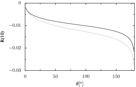
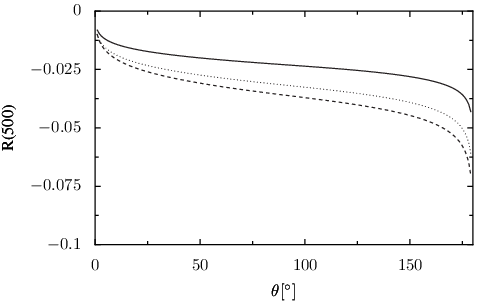
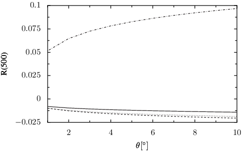
In Table 4 (Table 5) we show numerical values for the NNLO corrections to the differential cross section for a scattering angle θ=3∘\theta=3^{\circ} (θ=90∘\theta=90^{\circ}). In both tables we set ω=E/10\omega=E/\penalty 10. Finally, in Figure 4 we plot the ratio of the two-loop fermionic corrections to the tree-level cross section,

R⁡(s)=(απ)2​d​σNNLO+d​σγNLOd​σLOR(\sqrt{s})\,=\,\left(\frac{\alpha}{\pi}\right)^{2}\,\frac{d\sigma^{\rm{{\scriptscriptstyle{N}}{\scriptscriptstyle{N}}{\scriptscriptstyle{L}}{\scriptscriptstyle{O}}}}+d\sigma_{\gamma}^{\rm{{\scriptscriptstyle{N}}{\scriptscriptstyle{L}}{\scriptscriptstyle{O}}}}}{d\sigma^{\rm{{\scriptscriptstyle{L}}{\scriptscriptstyle{O}}}}} (4.13)

for s=10\sqrt{s}=10 GeV and s=500\sqrt{s}=500 GeV.

dσ\sigma //\penalty dΩ\Omega [nb] || s\sqrt{s} [GeV] 10 91 500
LO QED     [Eq. (2.5)] 440873 5323.91 176.349
LO Zfitter     [49, 50] 440875 5331.5 176.283
NNLO (ee)      [Eq. (4.6)] -1397.35 -35.8374 -1.88151
NNLO (e+μe\,+\,\mu)       “ -1394.74 -43.1888 -2.41643
NNLO (e+μ+τe\,+\,\mu\,+\tau)     “ -2.55179
NNLO photonic     [14, 16] 9564.09 251.661 12.7943
Table 4: Numerical values for the NNLO corrections to the differential cross section respect to the solid angle. Results are expressed in nanobarns for a scattering angle θ=3∘\theta=3^{\circ}. Empty entries are related to cases where the high-energy approximation cannot be applied.
dσ\sigma //\penalty dΩ\Omega [nb] || s\sqrt{s} [GeV] 10 91 500
LO QED     [Eq. (2.5)] 0.466409 0.00563228 0.000186564
LO Zfitter     [49, 50] 0.468499 0.127292 0.0000854731
NNLO (ee)      [Eq. (4.6)] -0.00453987 -0.0000919387 -4.28105 ⋅\cdot 10−610^{-6}
NNLO (e+μe\,+\,\mu)       “ -0.00570942 -0.000122796 -5.90469 ⋅\cdot 10−610^{-6}
NNLO (e+μ+τe\,+\,\mu\,+\tau)     “ -0.00586082 -0.000135449 -6.7059 ⋅\cdot 10−610^{-6}
NNLO (e+μ+τ+te\,+\,\mu\,+\tau+\,t)     “ -6.6927 ⋅\cdot 10−610^{-6}
NNLO photonic     [14, 16] 0.0358755 0.000655126 0.0000284063
Table 5: Numerical values for the NNLO corrections to the differential cross section respect to the solid angle. Results are expressed in nanobarns for a scattering angle θ=90∘\theta=90^{\circ}. Empty entries are related to cases where the high-energy approximation cannot be applied.
Refer to caption
Refer to caption
Figure 4: Ratio of the fermionic NNLO corrections to the differential cross section respect to the tree-level result for s=10\sqrt{s}=10 GeV and s=500\sqrt{s}=500 GeV. A solid line represents the electron-loop contributions, a dotted one the sum of electron- and muon-loop ones, and a dashed one includes also τ\tau leptons.
Refer to caption
Refer to caption
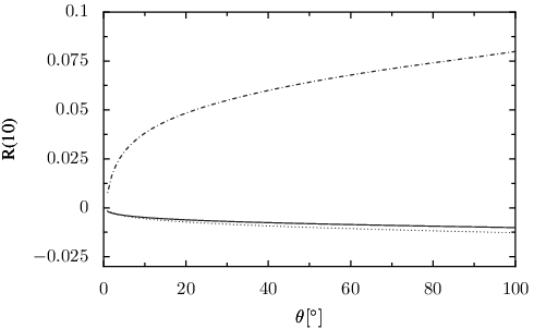
Figure 5: Same as Figure 4, including the photonic contributions of [2, 14, 16] (dash-dotted lines).

It is clear from the Tables, that although there is no decoupling of the heavier fermions (as indeed there shouldn’t, since the typical scale of the process is large compared to all the masses), the electron loop contributions dominate in the fermionic part and the latter is still substantially smaller than the pure photonic corrections.

5 Summary

In this article, we completed the computation of the virtual two-loop QED fermionic corrections to Bhabha scattering. Based on the kinematics of the targeted phenomenological applications, we considered the limit me2≪mf2≪s,t,um_{e}^{2}\ll m_{f}^{2}\ll s,t,u.

The fermionic double box contributions with two different mass scales have been derived for the first time here. Their numerical importance is comparable to the two-loop self-energies and vertices. We note, however, a qualitative difference. Due to the structure of the collinear singularities of the graphs, the contributions of the heavier fermions are not suppressed.

A numerical estimation of differential cross sections shows that the net fermionic two-loop effects may be neglected for applications at LEP 1 and LEP 2, but have to be taken into account for precision calculations when a level of 10−410^{-4} has to be reached, as is anticipated for the Giga-Z option of the ILC project.

Completing the NNLO program for Bhabha scattering requires still several ingredients. First, let us mention the contributions from the five light quark flavors. Here, an approach based on dispersion relations à la [51] should be suitable. On the other hand, the heavy top quark might be considered decoupling in a large part of the interesting kinematical regions. Furthermore, an implementation of the loop-by-loop corrections with pentagon diagrams has to be done.

Finally, light fermionic pair emission diagrams need to be considered. As known from the form-factor case, they are responsible for the cancellation of the leading part of the logarithmic sensitivity on the masses.
Exact and approximated results are made publicly available at [24]. The combination of our result with the photonic two-loop corrections of [16] and with electron loop corrections of  [17, 23] proves well-suited for phenomenogical purposes, e.g. a precise luminosity determination at a future International Linear Collider.

Acknowledgements

We would like to thank A. Arbuzov, R. Bonciani, A. Ferroglia and A. Penin for useful communications, and S. Moch and A. Mitov for interesting dicussions.

Work supported in part by Sonderforschungsbereich/Transregio TRR 9 of DFG ‘Computergestützte Theoretische Teilchenphysik’, by the Sofja Kovalevskaja Award of the Alexander von Humboldt Foundation sponsored by the German Federal Ministry of Education and Research, by the ToK Program “ALGOTOOLS” (MTKD-CD-2004-014319) by the Polish State Committee for Scientific Research (KBN), research projects in 2004–2005, and by the European Community’s Marie-Curie Research Training Networks MRTN-CT-2006-035505 ‘HEPTOOLS’ and MRTN-CT-2006-035482 ‘FLAVIAnet’.

Note added

We would like to thank T. Becher and K. Melnikov for drawing our attention to a problem with a first version of our result, which lead us to discover an incorrectly expanded integral. After correction, Eq. 4.9 agrees with the result published in the meantime in [53].

Appendix A Mass-Expanded Master Integrals

The list of Master Integrals required by our computation can already be found in Table V of [20]. The eight most difficult masters, those involving two different mass scales, have been derived in [42]. Because they are a substantial part of the present study we reproduce them here:

SE3l2M1m[on shell] =\displaystyle= M2m−4​ϵ{R[12​ϵ2+54​ϵ−38+ζ22+32L(R)−12L2(R)]\displaystyle M^{2}\ m^{-4\epsilon}\Bigl\{R\Bigl[\frac{1}{2\epsilon^{2}}+\frac{5}{4\epsilon}-\frac{3}{8}+\frac{\zeta_{2}}{2}+\frac{3}{2}L(R)-\frac{1}{2}L^{2}(R)\Bigr] (A.1)
+\displaystyle+ R2[1118−13L(R)]+ϵ[R(4516+54ζ2−ζ33−74L(R)+L2(R)\displaystyle R^{2}\Bigl[\frac{11}{18}-\frac{1}{3}L(R)\Bigr]+\epsilon\Bigl[R\Bigl(\frac{45}{16}+\frac{5}{4}\zeta_{2}-\frac{\zeta_{3}}{3}-\frac{7}{4}L(R)+L^{2}(R)
−\displaystyle- 12L3(R))+R2(−34+89L(R)−12L2(R))]},\displaystyle\frac{1}{2}L^{3}(R)\Bigr)+R^{2}\Bigl(-\frac{3}{4}+\frac{8}{9}L(R)-\frac{1}{2}L^{2}(R)\Bigr)\Bigr]\Bigr\},
SE3l2M1md[on shell] =\displaystyle= m−4​ϵ{12​ϵ2+12​ϵ[1+2L(R)]+12(1+ζ2)+L(R)+L2(R)\displaystyle m^{-4\epsilon}\Bigl\{\frac{1}{2\epsilon^{2}}+\frac{1}{2\epsilon}\Bigl[1+2L\left(R\right)\Bigr]+\frac{1}{2}\left(1+\zeta_{2}\right)+L\left(R\right)+L^{2}\left(R\right) (A.2)
+\displaystyle+ ϵ⁡[16​(3+3​ζ2−2​ζ3)+(1+ζ2)​L​(R)+L2​(R)+23​L3​(R)]\displaystyle\epsilon\Bigl[\frac{1}{6}\left(3+3\zeta_{2}-2\zeta_{3}\right)+\left(1+\zeta_{2}\right)L\left(R\right)+L^{2}\left(R\right)+\frac{2}{3}L^{3}\left(R\right)\Bigr]
+\displaystyle+ R⁡[−34+12​L​(R)+ϵ⁡(78−L⁡(R)+34​L2​(R))]\displaystyle R\Bigl[-\frac{3}{4}+\frac{1}{2}L(R)+\epsilon\left(\frac{7}{8}-L(R)+\frac{3}{4}L^{2}(R)\right)\Bigr]
+\displaystyle+ R2[−536+16L(R)+ϵ(−572+118L(R)+14L2(R))]},\displaystyle R^{2}\Bigl[-\frac{5}{36}+\frac{1}{6}L(R)+\epsilon\Bigl(-\frac{5}{72}+\frac{1}{18}L(R)+\frac{1}{4}L^{2}(R)\Bigr)\Bigr]\Bigr\},
V4l2M1m[x] =\displaystyle= m−4​ϵ{12​ϵ2+52​ϵ+12[19−3ζ2−Lm2(x)]\displaystyle m^{-4\epsilon}\Bigl\{\frac{1}{2\epsilon^{2}}+\frac{5}{2\epsilon}+\frac{1}{2}\Bigl[19-3\zeta_{2}-L_{m}^{2}(x)\Bigr] (A.3)
+\displaystyle+ M2x[−2+4ζ2−4ζ3−2Lm(x)+2LM(x)−4ζ2LM(x)\displaystyle\frac{M^{2}}{x}\Bigl[-2+4\zeta_{2}-4\zeta_{3}-2L_{m}(x)+2L_{M}(x)-4\zeta_{2}L_{M}(x)
+\displaystyle+ 2Lm(x)LM(x)−LM2(x)−Lm(x)LM(x)+LM3(x)]},\displaystyle 2L_{m}(x)L_{M}(x)-L_{M}^{2}(x)-L_{m}(x)L_{M}(x)+L_{M}^{3}(x)\Bigr]\Bigr\},
V4l2M1md[x] =\displaystyle= m−4​ϵm2{12​ϵ2+1ϵ[1+12Lm(x)]+2−ζ2+Lm(x)+14Lm2(x)\displaystyle\frac{m^{-4\epsilon}}{m^{2}}\Bigl\{\frac{1}{2\epsilon^{2}}+\frac{1}{\epsilon}\Bigl[1+\frac{1}{2}L_{m}(x)\Bigr]+2-\zeta_{2}+L_{m}(x)+\frac{1}{4}\,L_{m}^{2}(x) (A.4)
+\displaystyle+ M2x[1ϵ−1ϵLM(x)−1+3ζ2+Lm(x)+LM(x)\displaystyle\frac{M^{2}}{x}\Bigl[\frac{1}{\epsilon}-\frac{1}{\epsilon}L_{M}(x)-1+3\zeta_{2}+L_{m}(x)+L_{M}(x)
−\displaystyle- Lm(x)LM(x)−12LM2(x)]},\displaystyle L_{m}(x)L_{M}(x)-\frac{1}{2}L_{M}^{2}(x)\Bigr]\Bigr\},
V4l2M2m[x] =\displaystyle= m−4​ϵ​{12​ϵ2+1ϵ​[52+Lm​(x)]+12​(19+ζ2)+5​Lm​(x)+Lm2​(x)},\displaystyle m^{-4\epsilon}\Bigl\{\frac{1}{2\epsilon^{2}}+\frac{1}{\epsilon}\Bigl[\frac{5}{2}+L_{m}(x)\Bigr]+\frac{1}{2}(19+\zeta_{2})+5\ L_{m}(x)+L_{m}^{2}(x)\Bigr\}, (A.5)
V4l2M2md[x] =\displaystyle= m−4​ϵ6​x​[12​ζ3−6​ζ2​LM​(x)−LM3​(x)],\displaystyle\frac{m^{-4\epsilon}}{6x}\Bigl[12\zeta_{3}-6\zeta_{2}L_{M}(x)-L_{M}^{3}(x)\Bigr], (A.6)
B5l2M2m[x,y] =\displaystyle= m−4​ϵx{1ϵ2Lm(x)+1ϵ(−ζ2+2Lm(x)+12Lm2(x)+Lm(x)Lm(y))\displaystyle\frac{m^{-4\epsilon}}{x}\Bigl\{\frac{1}{\epsilon^{2}}L_{m}(x)+\frac{1}{\epsilon}\Bigl(-\zeta_{2}+2L_{m}(x)+\frac{1}{2}L_{m}^{2}(x)+L_{m}(x)L_{m}(y)\Bigr) (A.7)
−\displaystyle- 2​ζ2−2​ζ3+4​Lm​(x)+Lm2​(x)+13​Lm3​(x)−4​ζ2​Lm​(y)\displaystyle 2\zeta_{2}-2\zeta_{3}+4L_{m}(x)+L_{m}^{2}(x)+\frac{1}{3}L_{m}^{3}(x)-4\zeta_{2}L_{m}(y)
+\displaystyle+ 2​Lm​(x)​Lm​(y)+Lm​(x)​Lm2​(y)−16​Lm3​(y)\displaystyle 2L_{m}(x)L_{m}(y)+L_{m}(x)L_{m}^{2}(y)-\frac{1}{6}L_{m}^{3}(y)
−\displaystyle- (3​ζ2+12​Lm2​(x)−Lm​(x)​Lm​(y)+12​Lm2​(y))​ln⁡(1+yx)\displaystyle\Bigl(3\zeta_{2}+\frac{1}{2}L_{m}^{2}(x)-L_{m}(x)L_{m}(y)+\frac{1}{2}L_{m}^{2}(y)\Bigr)\ln\left(1+\frac{y}{x}\right)
−\displaystyle- (Lm(x)−Lm(y))Li2(−yx)+Li3(−yx)},\displaystyle\Bigl(L_{m}(x)-L_{m}(y)\Bigr)\text{Li}_{2}\left(-\frac{y}{x}\right)+\text{Li}_{3}\left(-\frac{y}{x}\right)\Bigr\},
B5l2M2md[x,y] =\displaystyle= m−4​ϵx​y{1ϵ[−Lm(x)Lm(y)+Lm(x)L(R)]−2ζ3+ζ2Lm(x)+4ζ2Lm(y)\displaystyle\frac{m^{-4\epsilon}}{xy}\Bigl\{\frac{1}{\epsilon}\Bigl[-L_{m}(x)L_{m}(y)+L_{m}(x)L(R)\Bigr]-2\zeta_{3}+\zeta_{2}L_{m}(x)+4\zeta_{2}L_{m}(y) (A.8)
−\displaystyle- 2​Lm​(x)​Lm2​(y)+16​Lm3​(y)−2​ζ2​L​(R)+2​Lm​(x)​Lm​(y)​L​(R)−16​L3​(R)\displaystyle 2L_{m}(x)L^{2}_{m}(y)+\frac{1}{6}L^{3}_{m}(y)-2\zeta_{2}L(R)+2L_{m}(x)L_{m}(y)L(R)-\frac{1}{6}L^{3}(R)
+\displaystyle+ (3​ζ2+12​Lm2​(x)−Lm​(x)​Lm​(y)+12​Lm2​(y))​ln⁡(1+yx)\displaystyle\Bigl(3\zeta_{2}+\frac{1}{2}L_{m}^{2}(x)-L_{m}(x)L_{m}(y)+\frac{1}{2}L_{m}^{2}(y)\Bigr)\ln\left(1+\frac{y}{x}\right)
+\displaystyle+ (Lm(x)−Lm(y))Li2(−yx)−Li3(−yx)}.\displaystyle\Bigl(L_{m}(x)-L_{m}(y)\Bigr)\text{Li}_{2}\left(-\frac{y}{x}\right)-\text{Li}_{3}\left(-\frac{y}{x}\right)\Bigr\}.

We list also the other expanded masters, including the correct normalizations. Note that, compared to the conventions employed in [20] and in Eq. (2.16), all integrals are rescaled by a factor mL⁡(D−2​l)m^{L(D-2l)}, where LL is the number of loops, D=4−2​ϵD=4-2\epsilon and ll is the number of internal lines. Expansions are performed up to the order required by our computation. For example, we include 𝒪⁡(m2){\cal O}(m^{2}) terms in SE2l2m[x] (see Eq. (A.10)) since the reduction procedure generates coefficients containing 1/m21/\penalty m^{2}. The same consideration applies to 𝒪⁡(ϵ){\cal O}(\epsilon) terms, which are included as long as the reduction brings inverse powers of ϵ\epsilon in the coefficient functions. Since in the following no ambiguities arise, in we drop the subscript ff and we set L(x)=ln(−m2/x)L(x)=\ln(-m^{2}/x),

T1l1m=(m2)1−ϵ​[1ϵ+ 1+ϵ⁡(1+ζ22)+ϵ2​(1+ζ22−ζ33)],\displaystyle\texttt{T1l1m}\,=\,(m^{2})^{1-\epsilon}\,\Bigl[\frac{1}{\epsilon}\,+\,1\,+\,\epsilon\,\Bigl(1+\frac{\zeta_{2}}{2}\Bigr)+\epsilon^{2}\Bigl(1+\frac{\zeta_{2}}{2}-\frac{\zeta_{3}}{3}\Bigr)\Bigr], (A.9)
SE2l2m[x] =\displaystyle= m−2​ϵ{1ϵ+ 2+L(x)+ 2m2x[ 1−L(x)]+ϵ[ 4−ζ22+ 2L(x)\displaystyle m^{-2\epsilon}\,\Bigl\{\frac{1}{\epsilon}\,+\,2\,+\,L(x)\,+\,2\,\frac{m^{2}}{x}\,\Bigl[\,1\,-\,L(x)\,\Bigr]\,+\,\epsilon\,\Bigl[\,4\,-\,\frac{\zeta_{2}}{2}\,+\,2\,L(x) (A.10)
+\displaystyle+ 12L2(x)+m2x( 2+ 2ζ2−L2(x))]+ϵ2[ 8−ζ2−73ζ3\displaystyle\,\frac{1}{2}\,L^{2}(x)\,+\,\frac{m^{2}}{x}\,\Bigl(\,2\,+\,2\,\zeta_{2}\,-\,L^{2}(x)\,\Bigr)\,\Bigr]\,+\,\epsilon^{2}\,\Bigl[\,8\,-\,\zeta_{2}\,-\,\frac{7}{3}\,\zeta_{3}
+\displaystyle+ 4​L​(x)−12​ζ2​L​(x)+L2​(x)+16​L3​(x)+m2x​( 2+ζ2CLOSE\displaystyle 4\,L(x)-\frac{1}{2}\,\zeta_{2}\,L(x)\,+\,L^{2}(x)\,+\,\frac{1}{6}\,L^{3}(x)\,+\,\frac{m^{2}}{x}\,\Bigl(\,2\,+\,\zeta_{2}
+\displaystyle+ 4ζ3+ζ2L(x)−13L3(x))]},\displaystyle 4\,\zeta_{3}\,+\,\zeta_{2}\,L(x)\,-\,\frac{1}{3}\,L^{3}(x)\Bigr)\Bigr]\Bigr\},
SE2l0m[x] =\displaystyle= m−2​ϵ{1ϵ+ 2+L(x)+ϵ[ 4−ζ22+ 2L(x)+12L2(x)]\displaystyle m^{-2\epsilon}\Bigl\{\frac{1}{\epsilon}\,+\,2\,+\,L(x)\,+\,\epsilon\,\Bigl[\,4\,-\,\frac{\zeta_{2}}{2}\,+\,2\,L(x)\,+\,\frac{1}{2}\,L^{2}(x)\,\Bigr] (A.11)
+\displaystyle+ ϵ2[8−ζ2−73ζ3+ 4L(x)−12ζ2L(x)+L2(x)+16L3(x)]},\displaystyle\epsilon^{2}\Bigl[8-\zeta_{2}\,-\,\frac{7}{3}\,\zeta_{3}\,+\,4\,L(x)\,-\,\frac{1}{2}\,\zeta_{2}\,L(x)\,+\,L^{2}(x)+\frac{1}{6}\,L^{3}(x)\,\Bigr]\Bigr\},
V3l1m[x]=m−2​ϵx​{4​ζ2+12​L2​(x)−ϵ⁡[−5​ζ3+ζ2​L​(x)−16​L3​(x)]},\displaystyle\texttt{V3l1m[x]}=\frac{m^{-2\epsilon}}{x}\,\Bigl\{4\,\zeta_{2}+\frac{1}{2}\,L^{2}(x)\,-\,\epsilon\Bigl[-5\,\zeta_{3}+\zeta_{2}\,L(x)-\frac{1}{6}\,L^{3}(x)\Bigr]\Bigr\}, (A.12)
SE3l1m[on shell] =\displaystyle= (m2)1−2​ϵ[12​ϵ2+54​ϵ+118+52ζ2+ϵ(−5516+254ζ2+113ζ3)\displaystyle(m^{2})^{1-2\epsilon}\Bigl[\frac{1}{2\,\epsilon^{2}}\,+\,\frac{5}{4\,\epsilon}\,+\,\frac{11}{8}\,+\,\frac{5}{2}\,\zeta_{2}\,+\,\epsilon\,\Bigl(\,-\,\frac{55}{16}\,+\,\frac{25}{4}\,\zeta_{2}\,+\,\frac{11}{3}\,\zeta_{3}\,\Bigr) (A.13)
+\displaystyle+ ϵ2(−94932+558ζ2+556ζ3+3038ζ4)],\displaystyle\epsilon^{2}\,\Bigl(\,-\,\frac{949}{32}\,+\,\frac{55}{8}\,\zeta_{2}\,+\,\frac{55}{6}\,\zeta_{3}\,+\,\frac{303}{8}\,\zeta_{4}\,\Bigr)\Bigr],
SE3l2m[x] =\displaystyle= (m2)1−2​ϵ{1ϵ2+1ϵ(3−x4​m2)+5+ζ2−L2(x)−xm2[138+12L(x)]\displaystyle(m^{2})^{1-2\epsilon}\Bigl\{\frac{1}{\epsilon^{2}}+\frac{1}{\epsilon}\Bigl(3-\frac{x}{4m^{2}}\Bigr)+5+\zeta_{2}-L^{2}(x)-\frac{x}{m^{2}}\Bigl[\frac{13}{8}+\frac{1}{2}L(x)\Bigr] (A.14)
+\displaystyle+ ϵ[ 3+ 3ζ2+163ζ3− 4L(x)+ 2ζ2L(x)− 3L2(x)−L3(x)\displaystyle\epsilon\,\Bigl[\,3\,+\,3\,\zeta_{2}\,+\,\frac{16}{3}\,\zeta_{3}\,-\,4\,L(x)\,+\,2\,\zeta_{2}\,L(x)\,-\,3\,L^{2}(x)\,-\,L^{3}(x)
−\displaystyle- xm2(11516−ζ24+134L(x)+12L2(x))]},\displaystyle\frac{x}{m^{2}}\,\Bigl(\,\frac{115}{16}\,-\,\frac{\zeta_{2}}{4}\,+\,\frac{13}{4}\,L(x)\,+\,\frac{1}{2}\,L^{2}(x)\,\Bigr)\,\Bigr]\Bigr\},
SE3l2md[x] =\displaystyle= m−4​ϵ{12​ϵ2+12​ϵ−12+ζ22−L(x)−12L2(x)−m2x[−2+L2(x)]\displaystyle m^{-4\epsilon}\Bigl\{\frac{1}{2\epsilon^{2}}+\frac{1}{2\epsilon}-\frac{1}{2}+\frac{\zeta_{2}}{2}-L(x)-\frac{1}{2}L^{2}(x)-\frac{m^{2}}{x}\Bigl[-2+L^{2}(x)\Bigr] (A.15)
+\displaystyle+ ϵ[−112+32ζ2+83ζ3−5L(x)+ζ2L(x)−2L2(x)−12L3(x)\displaystyle\epsilon\,\Bigl[-\frac{11}{2}+\frac{3}{2}\zeta_{2}+\frac{8}{3}\zeta_{3}-5L(x)+\zeta_{2}L(x)-2L^{2}(x)-\frac{1}{2}L^{3}(x)
−\displaystyle- m2x(−6ζ3− 4L(x)−2ζ2L(x)+L2(x)+L3(x))]}.\displaystyle\frac{m^{2}}{x}\,\Bigl(-6\,\zeta_{3}\,-\,4\,L(x)\,-2\,\zeta_{2}\,L(x)\,+\,L^{2}(x)\,+\,L^{3}(x)\Bigr)\Bigr]\Bigr\}.

Finally, the mass expanded one-loop box Master Integral B4l2m[x,y] can be collected from Eqs.(4.70)-(4.75) of [52]:

B4l2m[x,y] =\displaystyle= m−2​ϵx​y{2ϵ[L(y)−ln(xy)]+2L2(y)−2L(y)ln(xy)+ϵ[4ζ3−9ζ2L(y)\displaystyle\frac{m^{-2\epsilon}}{xy}\Bigl\{\frac{2}{\epsilon}\Bigl[L(y)-\ln\left(\frac{x}{y}\right)\Bigr]+2L^{2}(y)-2L(y)\ln\left(\frac{x}{y}\right)+\epsilon\Bigl[4\zeta_{3}-9\zeta_{2}L(y) (A.16)
+\displaystyle+ 23​L3​(y)+5​ζ2​ln⁡(xy)−L2​(y)​ln⁡(xy)+13​ln3⁡(xy)−6​ζ2​ln⁡(1+xy)\displaystyle\frac{2}{3}L^{3}(y)+5\zeta_{2}\ln\left(\frac{x}{y}\right)-L^{2}(y)\ln\left(\frac{x}{y}\right)+\frac{1}{3}\ln^{3}\left(\frac{x}{y}\right)-6\zeta_{2}\ln\left(1+\frac{x}{y}\right)
+\displaystyle+ 2​ln⁡(−xy)​ln⁡(xy)​ln⁡(1+xy)−ln2⁡(xy)​ln⁡(1+xy)\displaystyle 2\ln\left(-\frac{x}{y}\right)\ln\left(\frac{x}{y}\right)\ln\left(1+\frac{x}{y}\right)-\ln^{2}\left(\frac{x}{y}\right)\ln\left(1+\frac{x}{y}\right)
+\displaystyle+ 2ln(xy)Li2(1+xy)+2Li3(−xy)]}.\displaystyle 2\ln\left(\frac{x}{y}\right)\text{Li}_{2}\left(1+\frac{x}{y}\right)+2\text{Li}_{3}\left(-\frac{x}{y}\right)\Bigr]\Bigr\}.

References

  • [1] D. Bardin, W. Hollik, and T. Riemann, Z. Phys. C49 (1991) 485–490.
  • [2] A. Arbuzov, E. Kuraev, and B. Shaikhatdenov, Mod. Phys. Lett. A13 (1998) 2305–2316, hep-ph/9806215.
  • [3] Z. Bern, L. Dixon, and A. Ghinculov, Phys. Rev. D63 (2001) 053007, hep-ph/0010075.
  • [4] V. Smirnov, Phys. Lett. B460 (1999) 397–404, hep-ph/9905323.
  • [5] J. Tausk, Phys. Lett. B469 (1999) 225–234, hep-ph/9909506.
  • [6] F. Berends and R. Kleiss, Nucl. Phys. B228 (1983) 537.
  • [7] F. Berends, R. Kleiss, and W. Hollik, Nucl. Phys. B304 (1988) 712.
  • [8] S. Jadach, W. Placzek, E. Richter-Was, B. Ward, and Z. Was, Comput. Phys. Commun. 102 (1997) 229–251.
  • [9] S. Jadach, W. Placzek, and B. Ward, Phys. Lett. B390 (1997) 298–308, hep-ph/9608412.
  • [10] A. Arbuzov, G. Fedotovich, E. Kuraev, N. Merenkov, V. Rushai, and L. Trentadue, JHEP 10 (1997) 001, hep-ph/9702262.
  • [11] A. Arbuzov, G. Fedotovich, F. Ignatov, E. Kuraev, and A. Sibidanov, Eur. Phys. J. C46 (2006) 689–703, hep-ph/0504233.
  • [12] C. Carloni Calame, C. Lunardini, G. Montagna, O. Nicrosini, and F. Piccinini, Nucl. Phys. B584 (2000) 459–479, hep-ph/0003268.
  • [13] G. Balossini, C. Carloni Calame, G. Montagna, O. Nicrosini, and F. Piccinini, Nucl. Phys. B758 (2006) 227–253, hep-ph/0607181.
  • [14] N. Glover, B. Tausk, and J. van der Bij, Phys. Lett. B516 (2001) 33–38, hep-ph/0106052.
  • [15] A. Penin, Phys. Rev. Lett. 95 (2005) 010408, hep-ph/0501120.
  • [16] A. Penin, Nucl. Phys. B734 (2006) 185–202, hep-ph/0508127.
  • [17] R. Bonciani, A. Ferroglia, P. Mastrolia, E. Remiddi, and J. van der Bij, Nucl. Phys. B701 (2004) 121–179, hep-ph/0405275.
  • [18] R. Bonciani, A. Ferroglia, P. Mastrolia, E. Remiddi, and J. van der Bij, Nucl. Phys. B716 (2005) 280–302, hep-ph/0411321.
  • [19] R. Bonciani and A. Ferroglia, Phys. Rev. D72 (2005) 056004, hep-ph/0507047.
  • [20] M. Czakon, J. Gluza, and T. Riemann, Phys. Rev. D71 (2005) 073009, hep-ph/0412164.
  • [21] M. Czakon, J. Gluza, K. Kajda, and T. Riemann, Nucl. Phys. Proc. Suppl. 157 (2006) 16–20, hep-ph/0602102.
  • [22] M. Czakon, J. Gluza, and T. Riemann, Nucl. Phys. B751 (2006) 1–17, hep-ph/0604101.
  • [23] R. Bonciani and A. Ferroglia, Two-Loop QED Bhabha Scattering at
    http://pheno.physik.uni-freiburg.de/∼\simbhabha/.
  • [24] S. Actis, M. Czakon, J. Gluza and T. Riemann, Two-Loop QED Bhabha Scattering at http://www-zeuthen.desy.de/theory/research/bhabha/bhabha.html/.
  • [25] S. Actis, A. Ferroglia, G. Passarino, M. Passera, C. Sturm and S. Uccirati, GraphShot, a FORM package for automatic generation and manipulation of one and two loop Feynman diagrams, unpublished.
  • [26] P. Nogueira, J. Comput. Phys. 105 (1993) 279.
  • [27] P. Nogueira, An introduction to QGRAF 2.0, ftp://gtae2.ist.utl.pt/pub/qgraf/.
  • [28] M. Tentyukov and J. Fleischer, Comput. Phys. Commun. 132 (2000) 124–141, hep-ph/9904258.
  • [29] J. Vermaseren, New Features of FORM, math-ph/0010025.
  • [30] M. Czakon, DiaGen/IdSolver, unpublished.
  • [31] S. Laporta and E. Remiddi, Phys. Lett. B379 (1996) 283–291, hep-ph/9602417.
  • [32] S. Laporta, Int. J. Mod. Phys. A15 (2000) 5087–5159, hep-ph/0102033.
  • [33] E. Remiddi and J. Vermaseren, Int. J. Mod. Phys. A15 (2000) 725–754, hep-ph/9905237.
  • [34] T. Gehrmann and E. Remiddi, Nucl. Phys. B580 (2000) 485–518, hep-ph/9912329.
  • [35] T. Gehrmann and E. Remiddi, Nucl. Phys. B601 (2001) 248–286, hep-ph/0008287.
  • [36] S. Wolfram, The Mathematica book, Wolfram media/Cambridge University Press, 2003.
  • [37] N. Usyukina, Teor. Mat. Fiz. 22 (1975) 300–306.
  • [38] E. Boos and A. Davydychev, Theor. Math. Phys. 89 (1991) 1052–1063.
  • [39] M. Czakon, Comput. Phys. Commun. 175 (2006) 559–571, hep-ph/0511200.
  • [40] M. Roth and A. Denner, Nucl. Phys. B479 (1996) 495–514, hep-ph/9605420.
  • [41] S. Moch and P. Uwer, Comput. Phys. Commun. 174 (2006) 759–770, math-ph/0508008.
  • [42] S. Actis, M. Czakon, J. Gluza, and T. Riemann, Nucl. Phys. Proc. Suppl. 160 (2006) 91–100, hep-ph/0609051.
  • [43] G. ’t Hooft and M. Veltman, Nucl. Phys. B44 (1972) 189–213.
  • [44] C. Bollini and J. Giambiagi, Nuovo Cim. B12 (1972) 20–25.
  • [45] R. Bonciani, P. Mastrolia, and E. Remiddi, Nucl. Phys. B661 (2003) 289–343, hep-ph/0301170.
  • [46] P. Mastrolia and E. Remiddi, Nucl. Phys. B664 (2003) 341–356, hep-ph/0302162.
  • [47] R. Bonciani, P. Mastrolia, and E. Remiddi, Nucl. Phys. B676 (2004) 399–452, hep-ph/0307295.
  • [48] G. Burgers, Phys. Lett. B164 (1985) 167.
  • [49] D. Bardin, P. Christova, M. Jack, L. Kalinovskaya, A. Olchevski, S. Riemann, and T. Riemann, Comput. Phys. Commun. 133 (2001) 229–395, hep-ph/9908433.
  • [50] A. Arbuzov, M. Awramik, M. Czakon, A. Freitas, M. Grunewald, K. Monig, S. Riemann, and T. Riemann, Comput. Phys. Commun. 174 (2006) 728–758, hep-ph/0507146.
  • [51] B. Kniehl, M. Krawczyk, J. Kuhn, and R. Stuart, Phys. Lett. B209 (1988) 337.
  • [52] J. Fleischer, J. Gluza, A. Lorca, and T. Riemann, Eur. J. Phys. 48 (2006) 35–52, hep-ph/0606210.
  • [53] T. Becher and K. Melnikov, arXiv:0704.3582 [hep-ph].