Statistical properties of dust far-infrared emissionPreprint: Marc-Antoine Miville-Deschênes
Abstract
Context. Far-infrared dust emission has a self-similar structure which reveals the complex dynamical processes that shape the interstellar medium. The description of the statistical properties of this emission gives important constraints on the physics of the interstellar medium but it is also a useful way to estimate the contamination of diffuse interstellar emission in the cases where it is considered a nuisance.
Aims. The main goals of this analysis of the power spectrum and non-Gaussian properties of far-infrared dust emission are 1) to estimate the power spectrum of interstellar matter density in three dimensions, 2) to review and extend previous estimates of the cirrus noise due to dust emission and 3) to produce simulated dust emission maps that reproduce the observed statistical properties.
Methods. To estimate the statistical properties of dust emission we analyzed the power spectrum and wavelet decomposition of 100 m IRIS data (an improved version of the IRAS data) over 55 % of the sky. The simulation of realistic infrared emission maps is based on modified Gaussian random fields.
Results. The main results are the following. 1) The cirrus noise level as a function of brightness has been previously overestimated. It is found to be proportional to instead of , where is the local average brightness at 100 m. This scaling is in accordance with the fact that the brightness fluctuation level observed at a given angular scale on the sky is the sum of fluctuations of increasing amplitude with distance on the line of sight. 2) The spectral index of dust emission at scales between 5 arcmin and 12.5∘ is on average but shows significant variations over the sky. Bright regions have systematically steeper power spectra than diffuse regions. 3) The skewness and kurtosis of brightness fluctuations is high, indicative of strong non-Gaussianity. Unlike the standard deviation of the fluctuations, the skewness and kurtosis do not depend significantly on brightness, except in bright regions ( MJy sr-1) where they are systematically higher, probably due to contrasted structures related to star formation activity. 4) Based on our characterization of the 100 m power spectrum we provide a prescription of the cirrus confusion noise as a function of wavelength and scale. 5) Finally we present a method based on a modification of Gaussian random fields to produce simulations of dust maps which reproduce the power spectrum and non-Gaussian properties of interstellar dust emission.
Key Words.
Methods: statistical – ISM: structure – Infrared: ISM: continuum – dust1 Introduction
The interstellar medium emission shows fluctuations at all observable scales, revealing the self-similar nature of its density structure. The physical processes responsible for this self-similarity of the interstellar medium (ISM) structure is yet to be fully identified. It could be related to turbulent motions but also to chemical and thermal instabilities which trigger phase transitions and play an important role in shaping the medium.
Faced with the challenge to understand and characterize the great structural complexity of interstellar emission, astronomers have used several statistical tools (power spectrum, correlation and structure functions, wavelets, area-perimeter relation, principal component analysis,…) on several interstellar tracers : molecules Falgarone et al. 1991; Hobson 1992; Stutzki et al. 1998; Bensch et al. 2001; Brunt 2003; Padoan et al. 2003, atomic hydrogen Crovisier & Dickey 1983; Green 1993; Stanimirovic et al. 1999; Stanimirovic & Lazarian 2001; Dickey et al. 2001; Elmegreen et al. 2001; Miville-Deschênes et al. 2003a, extinction Padoan et al. 2002; Padoan et al. 2006 or dust emission Gautier et al. 1992; Abergel et al. 1996; Jewell 2001; Ingalls et al. 2004.


| 16.18 MJy sr-1 | |
| median | 3.49 MJy sr-1 |
| most probable | 2.51 MJy sr-1 |
| MJy sr-1 | 0.006% |
| MJy sr-1 | 0.06% |
| MJy sr-1 | 1.8% |
| MJy sr-1 | 11.6% |
| MJy sr-1 | 29.5% |
| MJy sr-1 | 61.1% |
| MJy sr-1 | 77.6% |
| MJy sr-1 | 89.2% |
| MJy sr-1 | 95.6% |
The analysis of the results of these tools is made difficult by projection, and instrumental effects but also by the fact that no observation is a perfect tracer of the total gas column density. Several works have been dedicated to the understanding of these effects Goldman 2000; Elmegreen et al. 2001; Padoan et al. 2001; Miville-Deschênes et al. 2003b and specifically on how one can retrieve the three-dimensional statistical properties of interstellar matter from astronomical observations. The recent theoretical progresses made in that area open interesting perspectives on the use of statistical tools to determine the three-dimensional structure of the gas and to identify privileged scales at which physical processes are important.
The characterization of the statistical properties of the interstellar emission is relevant for the understanding of the physics of the ISM but is also of importance for studies where interstellar emission is a nuisance. This is the case of the study of pre-stellar cores in molecular clouds but also of the analysis of the Cosmic Microwave Background (CMB) and Cosmic Infrared Background (CIB) radiations. In these cases the interstellar emission is considered as a noise (the so-called “cirrus noise”) for which one needs a detailed statistical description in order to remove it and account for it in the error budget. In that respect the interstellar medium is a rather complex noise source due to its highly non-white and non-Gaussian brightness fluctuations.
The present paper is a study of the power spectrum of interstellar dust emission at 100 m. The main goals are to use such analysis to put some constrains on the density structure of the interstellar medium but also to propose a caveat for estimation and simulation of cirrus noise. Gautier et al. 1992 showed that the power spectrum of the IRAS 100 m emission is characterized by a power law where the exponent is independant of the brightness. Moreover Gautier et al. 1992 showed that the normalisation factor of the power spectrum depends on the mean brightness of the region considered, with . This study has been conducted on a relatively small number of regions and at a time where the instrumental response of IRAS was not well known. In this paper we would like to revisit the work of Gautier et al. 1992 by extending it to the whole sky and by taking advantage of the recent reprocessing of the ISSA plates by Miville-Deschênes & Lagache 2005.
In § 2 we present the data used in this analysis. The results of the power spectrum analysis and the implication on the ISM density structure are presented in § 3. An estimate of the cirrus noise level in the FIR-submm is provided in § 4 and a method to produce realistic dust emission maps is given in § 5.

2 The IRAS survey and IRIS
In 1983 the Infrared Astronomical Satellite (IRAS) has made a survey of 98% of the sky in four bands : 12, 25, 60 and 100 m. Since then this dataset has been used extensively in almost all area of astrophysics. In the early 90s the IRAS team released the IRAS Sky Survey Atlas, a set of 430 fields with better calibration. Each field is a image with a pixel size of . Recently Miville-Deschênes & Lagache 2005 reprocessed the ISSA maps to correct for residual calibration defects and stripping. This new set of ISSA plates, named IRIS, improves significantly the quality of the IRAS data by lowering the noise level and improving the photometry of the four bands. Our analysis is based on the 100 m IRIS maps, available in native cartesian maps or in Healpix vector at http://www.cita.utoronto.ca/mamd/IRIS/.
One important parameter of our analysis is the estimate of the instrumental noise contribution to the power spectrum. We used only the IRIS maps for which we could compute the contribution of the noise. To do so we used the fact that the original ISSA plates are the combination of up to three HCON images. The power spectrum of the noise can be estimated by taking the power spectrum of the difference between two HCON images, as described in more details by Miville-Deschênes et al. 2002.
We selected only maps for which each pixel has been observed at least two times so that a noise map can be computed, which represent 236 maps (out of 430). Most maps of our sample have an average brightness lower than 20 MJy sr-1. This is representative of the whole sky statistics, as seen in Fig. 1 (see also Table 1) where the probability density function (PDF) and cumulative histogram of the 100 m brightness (CIB and zodiacal light subtracted) over the whole sky is presented. This figure, together with Table 1, show that 90 % of the sky has a brightness lower or equal to 20 MJy sr-1 (or cm-2 according to Lagache et al. 2000). This simple statistics of 100 m brightness reveals that there is less than 2 % of the sky with cm-2.

3 Power spectrum analysis
The power spectrum has been extensively used in the analysis of image structure. Working in Fourier (or spherical harmonics) space offers considerable advantages; this formalism allows for the quadratic separation of uncorrelated sources in the image (e.g., noise and signal) and deconvolution of the instrumental function. In addition working in Fourier space facilitates the comparison with numerical simulations of turbulent flows.
3.1 Computation of the power spectrum
The power spectrum of an image of Fourier Transform is computed from the amplitude defined as
| (1) |
The power spectrum is an angular average of between and where . The method we use to compute the power spectrum is the one described by Miville-Deschênes et al. 2002. To minimize edges effects in Fourier space we apodize the image, from which the mean was removed, using a cosine tapper of 15 pixels wide.
3.2 Contributions to the power spectrum
The main goal of our analysis is to characterize the power spectrum of the interstellar diffuse emission, but several astrophysical signals and artifacts may contribe to the power spectrum of the IRIS maps. The power spectrum of the IRIS maps may be formalized by the following equation:
| (2) |
where is the effective beam of the IRIS maps (which includes the instrumental beam and the map making), , , and are respectively the contributions of the interstellar medium, detected point sources, the unresolved CIB and the noise. All these contributions have to be estimated to characterize the interstellar component.
A typical power spectrum of a faint region of the sky is shown in Fig. 2. At large scales (low ), the power spectrum follows a power law ; this is the signature of the cirrus cloud emission Gautier et al. 1992. At smaller scales, the power spectrum flattens due to the combination of the noise, point sources and the CIB. These three components have a power spectrum signature that is flatter than the cirrus emission.
As stated in § 2, the power spectrum of the noise is estimated by taking the power spectrum of the difference between two HCON images. An example of a noise map and its power spectrum is shown in Fig. 1 of Miville-Deschênes et al. 2002. The power spectrum of the noise is well described by a power spectrum over most of the range.
To subtract the contribution of bright point sources we prefered to removed them directly in the IRIS maps prior to compute the power spectrum. To do so we used the point source extraction method described by Miville-Deschênes & Lagache 2005. For the CIB we assumed a flat power spectrum at the level determined by Miville-Deschênes et al. 2002 ( Jy2 sr-1 at 100 m). Like Miville-Deschênes et al. 2002 we made the assumption that the effective beam of the IRIS maps is Gaussian with a FWHM of 4.3 arcminutes.
3.3 Results
To obtain the spectral index of the dust emission in each IRIS map, we computed the power spectrum of the point source subtracted map and the power spectrum of the corresponding noise map. We then subtracted the noise power spectrum, divide the result by the Gaussian PSF and remove the CIB contribution.
Following what was done by Gautier et al. 1992 we have fitted the power spectrum of the Galactic emission in the range between and arcmin-1 using a power law:
| (3) |
where is the power spectrum value at arcmin-1. The power spectrum of the interstellar emission is in general very well fitted by such a power law.

3.3.1 Spectral index
The compilation of the power spectrum spectral index measured on our sample of 236 maps is shown in Fig. 3. The most probable spectral index is , in accordance with what was measured by Gautier et al. 1992. On the other hand, contrary to Gautier et al. 1992 who did their statistical analysis on only four regions, our larger sample allowed us to highlight a significant variation of the spectral index with the average brightness of the maps. Brighter regions on the sky tend to have a steeper power spectrum (see the lower panel of Fig. 3). The decrease of the spectral index with brightness can be approximated by:
| (4) |
where is the mean 100 m brightness of the map.

3.3.2 Normalisation
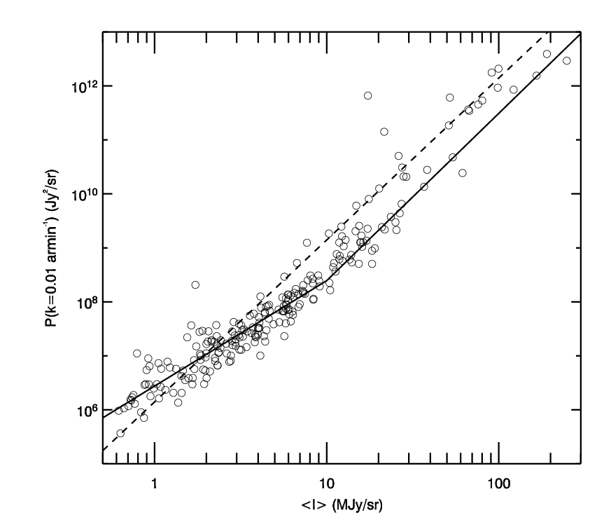
Regarding the normalization of the power spectrum Gautier et al. 1992 estimated that , where is the mean 100 m brightness at the 12.5∘ scale, given in MJy sr-1, and is in Jy2 sr-1. In Fig. 4 we present the variation of with for our sample, together with the relation of Gautier et al. 1992 (dashed line). The result of our analysis showed that the relation of Gautier et al. 1992 generally overestimates the fluctuation level at a given mean brightness. This discrepancy could be partly attributed to the fact that we used better calibrated IRAS data compare to the early IRAS product used by Gautier et al. 1992. On the other hand it is important to point out that the normalization relation given by Gautier et al. 1992 is compatible with the fact that they used only two faint ( MJy sr-1) and two bright regions ( MJy sr-1).
Using a much larger sample than Gautier et al. 1992 we found that the normalization of the power spectrum is better described by two regimes (solid line in Fig. 4): on % of the sky is proportional to instead of . For 10 MJy sr-1 we find
| (5) |
and for 10 MJy sr-1 we find
| (6) |
A similar trend was also observed by Jeong et al. 2005 using ISOPHOT observations (see their Fig. 12).
Another way of looking at the relation is to plot the standard deviation of each map as a function of (see Fig. 5). Here we made sure to remove quadratically the contribution of the instrumental noise and the CIB to each values of . Like for the power spectrum normalisation, two regimes are apparent in the vs relation with a transition around 10 MJy sr-1. Separating the data sample in two gives the following fits. for MJy sr-1:
| (7) |
and for MJy sr-1
| (8) |
3.4 Interpretation
3.4.1 Spectral index and density structure
Most spectral indexes measured here fall in the range between to . This is compatible with what was found by Wright 1998 () in a power spectrum analysis of the DIRBE data at 60, 100, 140 and 240 m on scales greater than 40 arcminutes. Other studies also estimated the equivalent of the power spectrum spectral index of the 100 m emission using the area-perimeter relation. Following Stutzki et al. 1998 there is a direct relation between the fractal dimension deduced from the area-perimeter relation () and the spectral index of the power spectrum ():
| (9) |
Bazell & Desert 1988 and Dickman et al. 1990 measured (corresponding to ) for relatively bright regions at 100 m ( MJy sr-1). These values of are rather high (steep power spectrum) but not incompatible with our analysis. In a similar analysis on fainter regions Vogelaar & Wakker 1994 measured , corresponding to which is very similar to our results.
The interpretation of these results in terms of the density structure of the ISM and the comparison with what is deduced from gas tracers can only be done by considering a model for the 100 m emission. At this wavelength the interstellar emission is dominated by the grey body emission from big dust grains at thermal equilibrium with the radiation field Desert et al. 1990. For a given model of the composition of dust grain Desert et al. 1990; Li & Draine 2001 the conversion of 100 m brightness to gas column density depends on the gas/dust mass ratio (known to be rather constant in the ISM) and on the big grain equilibrium temperature. The big grain equilibrium temperature is related to the local radiation field strength and spectrum which depends on the presence or not of nearby heating sources and on the extinction. Variation of the dust equilibrium temperature can also occur locally due to variation of the grain structure which can affect their emissivity11 1 Aggregation of small dust particles on bigger grains can increase significantly their area / mass ratio which leads to a more efficient cooling of the grains. See Stepnik et al. 2003 for a striking example of this effect..
In diffuse regions of the sky at high Galactic latitudes, far from star-forming regions, clouds are optically thin to stellar radiation, and the radiation field is uniform which result in very limited variations of dust equilibrium temperature. Localised variations of the dust grain temperature were observed in cirrus clouds Bernard et al. 1999, but overall several studies Boulanger & Pérault 1988; Boulanger et al. 1996 showed a strong correlation between the 100 m micron and the hydrogen column density which is in favor of a rather uniform gas/dust ratio and limited variations of the dust temperature. Based on these results we believe that the 100 m micron can not be used as a perfect surrogate for gas column density but overall it does not introduce a systematic bias in the determination of the column density power spectrum. In this context, and considering that the power spectrum of the column density gives directly the power spectrum of the density structure Miville-Deschênes et al. 2003b, we consider that the values measured here in the diffuse regions (for 10 MJy sr-1) are typical of the spectral index of the density field in three dimensions in the solar neighborhood.
In bright regions ( MJy sr-1) the power spectrum is observed to be significantly steeper (Fig 3). A steepening of the power spectrum with brightness was also found by Kiss et al. 2003 on 90-200 m ISOPHOT observations. We observed that this steepening coincides with a departure from the relation (see Fig. 4) and a systematic increase of the skewness and kurtosis of the brightness fluctuations (see Fig. 11). This variation of with might reflect, at least in part, local variations of the density power spectrum. It could also be attributed to the effect of gravity or anisotropic radiation fields which would both increase the large scale coherence (like in star forming regions or at Galactic scale in the plane) and therefore steepen the power spectrum of the 100 m emission. The effect of extinction in these parts of the sky will also induce important dust temperature variations which will affect the power spectrum. These effects will certainly have an impact on the observed brightness fluctuations and make the interpretration of the power spectrum difficult.
To compare the results obtained here with statistical analysis of gas emission, it is important to point out that the 100 m emission traces all the interstellar components: atomic, molecular and ionized gas. Gas observations (21 cm and CO) showed that diffuse and dense gas have different density structure. In general regions of cold and dense gas have stronger small scale fluctuations (and therefore a flatter density power spectrum - see for instance Stutzki et al. 1998 who measured on CO observations of the Polaris flare, a dense cirrus cloud with a significant fraction of molecular gas) than regions of diffuse gas (Miville-Deschênes et al. 2003a measured on 21 cm observations of a diffuse cirrus cloud). This behavior seems also in accordance with numerical simulations (see Audit & Hennebelle 2005 for instance).
This could reflect the fact that molecular tracers like CO reveal only the density structure of dense regions and miss the more diffuse and large scale structure of molecular clouds. In that respect dust emission would be a more reliable tracer of the global density structure of the ISM as the observed spectral index at 100 m is a weighted mean of the various contributions from dense and diffuse media on the line of sight. One striking example of that comes from the direct comparison of infrared and 21 cm emission in high-latitude clouds where dust emission usually shows stronger brightness fluctuations at small scale than Hi, this being attributed to the presence of localized molecular regions (see for instance Joncas et al. 1992).
3.4.2 The relation
Here we would like to propose one interpretation for the scaling of the power spectrum normalization (or equivalently the brightness standard deviation ) with average brightness (equations 5 and 7).
Lets consider a three-dimensional scalar field , which could be a dust emissivity field, of size on the plane of the sky and of depth . In the case of constant dust temperature and neglecting opacity effects, the projection of this 3D field on 2D would correspond to a dust emission map:
| (10) |
What would be the relation between the average and standard deviation of the projected brightness for such a field ? The average brightness of the dust map is simply
| (11) |
where is the volume averaged of .
On the other hand to compute the standard deviation of the dust map () one should consider that brightness fluctuations are added quadratically along the line of sight. Each slice of the cube contributes to :
| (12) |
Combined with Eq. 11 this leads to
| (13) |
which is not what is observed.
Cartesian coordinates used in the previous demonstration is in fact not a realistic representation when it comes to estimate . In fact, with the increase of the depth of the line of sight , a given angular scale on the sky corresponds to increasing physical size : .
In the integral of Eq. 12 we made the assumption that is the standard deviation at scale . In fact we should have taken into account that varies with . For a power spectrum following a power law () the variance of brightness fluctuations as a function of scale is Brunt & Heyer 2002:
| (14) |
Therefore we can rewrite Eq. 12
| (15) |
which leads to
| (16) | |||||
There are two important results to extract from the previous equation. First the fact that we observed structure of increasing physical size with at a given angular scale does not modify the slope of the power law for : both and have the same spectral index . Secondly the dependence of on is now related to the spectral index . For a typical value of we obtain which is exactly the observed relation for MJy sr-1.
For larger the departure from a simple can be explained partly because the spectral index decreases but most of all it is important to notice that brightness fluctuations become highly non-Gaussian (high skewness and kurtosis - see Fig. 11). In this regime the standard deviation becomes significantly affected by non-Gaussian fluctuations which could be related to localized star forming regions in the image.

4 Cirrus noise
In this section we use the properties of the power spectrum of 100 m emission to estimate the level of cirrus confusion noise of dust emission.
4.1 Brightness fluctuations
To estimate the level of fluctuations as a function of scale and brightness it is convenient to use the real-space representation given by Eq. 14, as opposed to a Fourier one. Using the value of measured at (see equations 7 and 8) we can normalize Eq. 14 and estimate the level of brightness fluctuation of interstellar dust (in MJy sr-1) at scale (in degree) and wavelength . For the two regimes identified in this study (lower and higher than =10 MJy sr-1) we have the following relations:
| (17) |
and
| (18) |
where is in MJy sr-1, is given by Eq. 4 and is an estimate of the dust brightness ratio at wavelength and 100 m. Such ratio can be estimated using a grey body model like the one of Desert et al. 1990
| (19) |
where is the Planck function at grain temperature and is the dust emissivity index. Typical values in the diffuse ISM for the dust temperature and emissivity index are K and . In the sub-millimeter and millimeter ranges the dust emission departs from this simple model and one might want to use a combination of two dust components (see Finkbeiner et al. 1999 for an example of such model).


4.2 Noise per beam
Equations 17 and 18 give the surface brightness fluctuation level of dust at any scale, brightness and wavelength. One useful specific case to consider is the contribution of cirrus noise at the scale of an instrument beam, to estimate the effective point source detection level for instance. Following Helou & Beichman 1990 and Gautier et al. 1992 we consider the cirrus noise level at a scale two times the beam size (i.e., , where is the beam FWHM). This noise level (in mJy/beam) at wavelength is simply
| (20) |
where is the beam in steradian
| (21) |
and is in degrees. The cirrus noise in mJy/beam is then given by
| (22) |
and
| (23) |
where is still given by Eq. 4.
These relations can be compared with the prescription of Helou & Beichman 1990 often used to estimate cirrus confusion noise. These authors considered the situation where the beam of the instrument is given by the diffraction limit of a telescope of diameter . In this case .
The comparison between our estimate of the cirrus noise and the one given by Helou & Beichman 1990 for a 1m telescope at 100 m is shown in Fig 7. The difference is important in several aspects. First at low brightness the slopes of are very different, due to the regime revealed in our study. The change of slope has the implication that our estimate of the cirrus noise in low brightness regions is much higher. This is also due to the flattening of the power spectrum index at low brightness. On the other hand our cirrus noise estimate is much lower than the estimate of Helou & Beichman 1990 at large brightness. This effect is caused by the fact that we observe steeper power spectra in bright regions. Therefore the brightness fluctuations are much smaller when extrapolated to small scale.
4.3 Limitation
The prescriptions given here to estimate the level of cirrus noise is only indicative. It would be strictly correct for a Gaussian field which is not the case of interstellar emission. As it will be described in more details in the next section, dust emission has non-Gaussian brightness fluctuations at all scales. For the sake of data interpretation, confusion estimate or tests of component separation algorithms (including point source extraction) it is useful to produce realistic simulations of dust emission maps with proper non-Gaussian properties. It is the topic of the next section.

5 Construction of artificial dust emission maps
5.1 Fractional Brownian motion
Fractional Brownian motions (fBm, also known as Gaussian random fields) are often used to simulate interstellar emission (Stutzki et al. 1998; Miville-Deschênes et al. 2003b, e.g.,). By construction such objects can reproduce the power spectrum of any image, with the limitation that its phase is random. A comparison of a typical IRIS map and a fBm with the same power spectrum is given in Fig. 6. The fBm reproduces well the self-similar structure of the interstellar emission. On the other hand the fBm seems smoother and less contrasted than the observation.
Because of the Gaussian nature of their fluctuations, fBms with positive values only can’t have a large contrast. If we define the contrast of a map as , positive fBms are restricted to as the average needs to be greater than to have only positive values22 2 or equivalently that 99 % of the values are between and .. This can be compared with the contrast of real IRIS map given in Fig. 8, where we used (i.e., the standard deviation at a scale of 12.5∘). The median contrast is 0.3 which indicate the limitation of the use of fBms used to simulate realistic infrared dust maps. In addition one would notice that the contrast increases significantly with brightness and especially for greater than 10 MJy sr-1, in accordance with equations 7 and 8. In addition, will increase with scale as depends on scale (according to Eq. 14) but not (at high Galactic latitude). Based only on the contrast, the use of fBm becomes limited to small (a few degrees) and faint regions of the sky.
5.2 Wavelet decomposition
Apart from the global contrast limitation, there is a fundamental difference between fBms and observations which is related to the non-Gaussian properties of the interstellar emission. The brightness fluctuations seen in infrared dust maps show contrasted structures, often filaments, that reflect their non-Gaussian nature. Using a wavelet decomposition of 100 m maps, Jewell 2001 showed clearly that, contrary to random-phase realisations, the histograms of brightness fluctuations at a given scale are highly non-Gaussian. Abergel et al. 1996 and Aghanim et al. 2003 gave also striking examples of that. Wavelet transforms are powerful tools to study the statistical moments higher than two and estimate the non-Gaussian properties of images Aghanim et al. 2003. They complement the power spectrum analysis which gives only the variation of the second moment - the standard deviation - with scale.
To illustrate that we present in figures 9 and 10 the wavelet decomposition obtained using the “a trou” algorithm Starck & Murtagh 1998 for the IRIS and fBm maps of Fig. 6. As expected the distribution of brightness fluctuations at a given scale are Gaussian for fBms (see Fig. 10). On the other hand the distribution of wavelet coefficients of an IRIS map (see Fig. 9) follows an asymmetrical distribution with exponential wings, which results in significant skewness and kurtosis.
In Fig. 11 are compiled the skewness and kurtosis of the wavelet coefficients found for all 236 maps of our sample, for scales from pixels (12 arcmin) to 32 pixels (48 arcmin). There is a not a strong correlation of the skewness and kurtosis with brightness, unlike for the standard deviation (Fig. 5). There is a slight increase of skewness and kurtosis at small scale and low brightness that should be attributed to noise and CIB 33 3 Both processes being more Gaussian than the interstellar emission they have the effect of lowering the skewness and kurtosis mostly. This effect is more important at small scale and low brightness where the noise and CIB fluctuations are stronger with respect to interstellar fluctuations.. On the other hand one would note a sharp increase of the skewness and kurtosis for MJy sr-1.
Finally, apart from the global difference of the wavelet coefficient distribution between fBms and observations, one would notice that brightness fluctuations at a given scale in the IRIS map are generally greater in bright regions of the map, contrary to the fBm where the amplitude of fluctuations at a given scale is independent of position. This just reflects the fact that brightness fluctuations are generally stronger in bright region, in accordance with equations 7 and 8. By construction fBms do not behave like that; the amplitude of fluctuations is uniform and independant of local variations of the average brightness.


5.3 Non-Gaussian fBm
In this section we propose a method to modify fBms such that they better reproduce the statistical properties of the infrared emission. We want to produce simulations of dust emission maps that would satisfy a given number of assumptions:
- 1.
Positive values only
- 2.
Power spectrum following a power law :
- 3.
Greater brightness fluctuations in bright regions (following ).
Several attempts have been made to generate non-Gaussian maps, especially to produce non-Gaussian realizations of the Cosmic Microwave Background (CMB) Vio et al. 2001; Vio et al. 2002; Rocha et al. 2005. In general these methods involve a modification of a Gaussian realization but they don’t comply with all our requirements. Especially in the context of the CMB there is no need to produce maps with only positive values and to have stronger brightness fluctuations in bright regions.
Here is how we proceeded to construct a non-Gaussian fBm map with the same statistical properties as an IRIS map and with only positive values. The method presented here is similar to the one used by Elmegreen 2002; Brunt & Heyer 2002. First we generate a classical fBm with same standard deviation as map . We add an offset to force all values to be positives and to be as close as possible to the average of . We then create a modified fBm such that:
| (24) |
and such that has the same average, standard deviation and skewness than and only positive values. The parameters , and are thus constrained iteratively so to match the first three statistical moments of the map . Such a modified fBm is shown in Fig. 6 and its wavelet decomposition in Fig. 12. The effect of the exponent is to produce greater fluctuations in bright regions, in accordance with the observations. The wavelet decomposition is quite illustrative in that respect. In particular the histograms of wavelet coefficients are almost impossible to discriminate from the ones of the IRIS map.
The key parameter in this transformation is which control the amount of non-Gaussianity introduced in the map. We did such a simulation for each of the 236 maps of our sample and the results are summarized in Fig. 13. One would note the scaling of with skewness , which clearly indicate the impact of that parameter on the non-Gaussianity of the map. The median value of is (see Fig. 13).
Even though it reproduces very well several statistical properties of the observed emission, it is important to note that one important limitation of this method is that it produces only isotropic fluctuations and failed to reproduce to filamentary structure of the ISM.
5.4 Extend an image to smaller scales
To estimate the capabilities and performances of some instruments at observing diffuse interstellar emission it is often needed to extrapolate low resolution observations to smaller angular scales. One example of that would be the estimate of the diffuse emission structure that will be observed at a scale of 8 arcsec by Herschel-PACS given the IRAS data at 5 arcmin resolution. In this context it is useful to produce constrained realisations of the interstellar diffuse emission based on low resolution observations. The statistical analysis presented here provides a theoretical basis () on which to add small scales using larger scale informations.
Given a low resolution map characterized by a beam , a higher resolution of beam can be computed using the following method:
| (25) |
where is a classical positive fBm map, and , and are determined as described in the previous section. In the previous equation the difference extends the structure up to the higher resolution beam . The modulation of the small scale fluctuations by assures that they follow the relation.

6 Conclusion
In this paper we presented an analysis of the power spectrum and wavelet decomposition of the IRIS/IRAS 100 m emission over 55 % of the sky. The main goals of this work were 1) to review and extend the study of Gautier et al. 1992 using better calibrated IRAS maps, estimates of the noise and CIB contributions and a larger sample, 2) provide a more precise prescription for cirrus noise and 3) suggest a technique to simulate dust emission map with proper statistical properties.
We found an average spectral index () compatible with Gautier et al. 1992 () but with a significant variation from to . Considering that 100 m emission is a relatively reliable tracer of column density in faint regions, these values of should be representative of the spectral index of density in three dimensions in the local interstellar medium. The comparison with other tracers leads to the conclusion that there is most probably a significant contribution from cold gas to the brightness fluctuations observed. We also found a slight variation of with which could be explained by the impact of gravity or spatial variations of dust temperature in star forming regions.
We also found that the amplitude of the brightness fluctuations were generally overestimated by Gautier et al. 1992. In regions with a 100 m average brightness lower than 10 MJy sr-1 the brightness fluctuation level is proportional to and not as stated by Gautier et al. 1992. We showed that this behavior can be explained by the fact that the brightness fluctuation level observed at a given angular size on the sky is the sum of fluctuations of increasing amplitude with distance.
This detailed description of the power spectrum properties of the 100 m emission allowed us to determine a new prescription of the cirrus confusion noise in the far-infrared and sub-millimeter as a function of column density and scale. On the other hand we stressed that this cirrus noise estimate relies on the hypothesis of Gaussian fluctuations, which is clearly not the case for interstellar emission. In that context we proposed a method to modify Gaussian random fields such that it reproduces the power spectrum but also the level of non-Gaussianity observed which is related to the fact that bright regions have stronger brightness fluctuations than faint ones. Such images could be used to tests component separation algorithms (including point source extraction) that have to deal with non-Gaussian components. The main limitation of the technique we propose is that it does not reproduce the obvious filamentarity seen in observations.
Some of the results in this paper have been obtained using the HEALPix package Gorski et al. 2005. This work was supported by the Canadian Space Agency. It is a pleasure to thank J. Richard Bond for enlightening discussions.
References
- Abergel et al. (1996) Abergel, A., Boulanger, F., Delouis, J. M., Dudziak, G. & Steindling, S. 1996, A&A, 309, 245.
- Aghanim et al. (2003) Aghanim, N., Kunz, M., Castro, P. G. & Forni, O. 2003, A&A, 406, 797–816.
- Audit & Hennebelle (2005) Audit, E. & Hennebelle, P. 2005, A&A, 433, 1–13.
- Bazell & Desert (1988) Bazell, D. & Desert, F. X. 1988, ApJ, 333, 353.
- Bensch et al. (2001) Bensch, F., Stutzki, J. & Ossenkopf, V. 2001, A&A, 366, 636.
- Bernard et al. (1999) Bernard, J. P., Abergel, A., Ristorcelli, I., Pajot, F., Torre, J. P., Boulanger, F., Giard, M., Lagache, G., Serra, G., Lamarre, J. M., Puget, J. L., Lepeintre, F. & Cambrésy, L. 1999, A&A, 347, 640.
- Boulanger & Pérault (1988) Boulanger, F. & Pérault, M. 1988, ApJ, 330, 964.
- Boulanger et al. (1996) Boulanger, F., Abergel, A., Bernard, J. P., Burton, W. B., Desert, F. X., Hartmann, D., Lagache, G. & Puget, J. L. 1996, A&A, 312, 256.
- Brunt & Heyer (2002) Brunt, C. M. & Heyer, M. H. 2002, ApJ, 566, 276.
- Brunt (2003) Brunt, C. M. 2003, ApJ, 583, 280.
- Crovisier & Dickey (1983) Crovisier, J. & Dickey, J. M. 1983, A&A, 122, 282.
- Desert et al. (1990) Desert, F. X., Boulanger, F. & Puget, J. L. 1990, A&A, 237, 215.
- Dickey et al. (2001) Dickey, J. M., McClure-Griffiths, N. M., Stanimirovic, S., Gaensler, B. M. & Green, A. J. 2001, ApJ, 561, 264.
- Dickman et al. (1990) Dickman, R. L., Margulis, M. & Horvath, M. A. 1990, ApJ, 365, 586.
- Elmegreen et al. (2001) Elmegreen, B. G., Kim, S. & Staveley-Smith, L. 2001, ApJ, 548, 749.
- Elmegreen (2002) Elmegreen, B. G. 2002, ApJ, 564, 773.
- Falgarone et al. (1991) Falgarone, E., Phillips, T. G. & Walker, C. K. 1991, ApJ, 378, 186.
- Finkbeiner et al. (1999) Finkbeiner, D. P., Davis, M. & Schlegel, D. J. 1999, ApJ, 524, 867.
- Gautier et al. (1992) Gautier, T. N. I., Boulanger, F., Perault, M. & Puget, J. L. 1992, AJ, 103, 1313.
- Goldman (2000) Goldman, I. 2000, ApJ, 541, 701.
- Gorski et al. (2005) Gorski, K. M., Hivon, E., Banday, A. J., Wandelt, B. D., Hansen, F. K., Reinecke, M. & Bartelmann, M. 2005, ApJ, 622, 759–771.
- Green (1993) Green, D. A. 1993, MNRAS, 262, 327.
- Hauser et al. (1998) Hauser, M. G., Arendt, R. G., Kelsall, T., Dwek, E., Odegard, N., Weiland, J. L., Freudenreich, H. T., Reach, W. T., Silverberg, R. F., Moseley, S. H., Pei, Y. C., Lubin, P., Mather, J. C., Shafer, R. A., Smoot, G. F., Weiss, R., Wilkinson, D. T. & Wright, E. L. 1998, ApJ, 508, 25–43.
- Helou & Beichman (1990) Helou, G. & Beichman, C. A. The confusion limits to the sensitivity of submillimeter telescopes. In ESA, editor, From Ground-Based to Space-Borne Sub-mm Astronomy, page 117, 1990.
- Hobson (1992) Hobson, M. P. 1992, MNRAS, 256, 457.
- Ingalls et al. (2004) Ingalls, J. G., Miville-Deschênes, M. A., Reach, W. T., Noriega-Crespo, A., Carey, S. J., Boulanger, F., Stolovy, S. R., Padgett, D. L., Burgdorf, M. J., Fajardo-Acosta, S. B., Glaccum, W. J., Helou, G., Hoard, D. W., Karr, J., O’Linger, J., Rebull, L. M., Rho, J., Stauffer, J. R. & Wachter, S. 2004, Astrophysical Journal Supplement Series, 154, 281–285.
- Jeong et al. (2005) Jeong, W. S., Mok Lee, H., Pak, S., Nakagawa, T., Minn Kwon, S., Pearson, C. P. & White, G. J. 2005, MNRAS, 357, 535–547.
- Jewell (2001) Jewell, J. 2001, ApJ, 557, 700.
- Joncas et al. (1992) Joncas, G., Boulanger, F. & Dewdney, P. E. 1992, ApJ, 397, 165.
- Kiss et al. (2003) Kiss, C., Abraham, P., Klaas, U., Lemke, D., Heraudeau, P., Burgo, C. D. & Herbstmeier, U. 2003, A&A, 399, 177.
- Lagache et al. (2000) Lagache, G., Haffner, L. M., Reynolds, R. J. & Tufte, S. L. 2000, A&A, 354, 247.
- Li & Draine (2001) Li, A. & Draine, B. T. 2001, ApJ, 554, 778–802.
- Miville-Deschênes & Lagache (2005) Miville-Deschênes, M. A. & Lagache, G. 2005, Astrophysical Journal Supplement Series, 157, 302–323.
- Miville-Deschênes et al. (2002) Miville-Deschênes, M. A., Lagache, G. & Puget, J. L. 2002, A&A, 393, 749.
- Miville-Deschênes et al. (2003a) Miville-Deschênes, M. A., Joncas, G., Falgarone, E. & Boulanger, F. 2003a, A&A, 411, 109.
- Miville-Deschênes et al. (2003b) Miville-Deschênes, M. A., Levrier, F. & Falgarone, E. 2003b, ApJ, 593, 831.
- Padoan et al. (2001) Padoan, P., Rosolowsky, E. W. & Goodman, A. A. 2001, ApJ, 547, 862.
- Padoan et al. (2002) Padoan, P., Cambrésy, L. & Langer, W. 2002, ApJ, 580, L57.
- Padoan et al. (2003) Padoan, P., Goodman, A. A. & Juvela, M. 2003, ApJ, 588, 881.
- Padoan et al. (2006) Padoan, P., Cambrésy, L., Juvela, M., Kritsuk, A., Langer, W. D. & Norman, M. L. 2006, ApJ, 649, 807–815.
- Rocha et al. (2005) Rocha, G., Hobson, M. P., Smith, S., Ferreira, P. & Challinor, A. 2005, MNRAS, 357, 1–11.
- Stanimirovic & Lazarian (2001) Stanimirovic, S. & Lazarian, A. 2001, ApJ, 551, L53.
- Stanimirovic et al. (1999) Stanimirovic, S., Staveley-Smith, L., Dickey, J. M., Sault, R. J. & Snowden, S. L. 1999, MNRAS, 302, 417.
- Starck & Murtagh (1998) Starck, J. L. & Murtagh, F. 1998, Publications of the Astronomical Society of the Pacific, 110, 193.
- Stepnik et al. (2003) Stepnik, B., Abergel, A., Bernard, J. P., Boulanger, F., Cambrésy, L., Giard, M., Jones, A. P., Lagache, G., Lamarre, J. M., Meny, C., Pajot, F., Peintre, F. L., Ristorcelli, I., Serra, G. & Torre, J. P. 2003, A&A, 398, 551.
- Stutzki et al. (1998) Stutzki, J., Bensch, F., Heithausen, A., Ossenkopf, V. & Zielinsky, M. 1998, A&A, 336, 697.
- Vio et al. (2001) Vio, R., Andreani, P. & Wamsteker, W. 2001, Publications of the Astronomical Society of the Pacific, 113, 1009–1020.
- Vio et al. (2002) Vio, R., Andreani, P., Tenorio, L. & Wamsteker, W. 2002, Publications of the Astronomical Society of the Pacific, 114, 1281–1289.
- Vogelaar & Wakker (1994) Vogelaar, M. G. R. & Wakker, B. P. 1994, A&A, 291, 557.
- Wright (1998) Wright, E. L. 1998, ApJ, 496, 1.