Symmetry properties of the nodal superconductor PrOs4Sb12
Abstract
We present a theoretical study of the superconducting gap function in PrOs4Sb12 using a symmetry-based approach. A three-component order parameter in the triplet channel best describes superconductivity. The gap function is non-degenerate and the lower branch has four cusp nodes at unusual points of the Fermi surface, which lead to power law behaviours in the density of states, specific heat and nuclear spin relaxation rate.
pacs
74.20.-z, 71.27.+a, 71.10.-wI Introduction
By most accounts, PrOs4Sb12 is an unconventional superconductor.Maple2001; Bauer2002; Izawa2003; Aoki2003; Chia2003; Huxley2004; Frederick2005; Nishiyama2005; Higemoto2007 The superconducting phase breaks time-reversal symmetryAoki2003 and the paired electrons are in a spin triplet configuration.Higemoto2007 The existence of point nodes in the superconducting gap function is indicated by power law behaviour in the temperature dependencies of specific heat,Bauer2002; Frederick2005 penetration depth,Chia2003 thermal conductivityIzawa2003, and Sb-NQR; Katayama2007 however other experiments find the gap function to be nodeless.MacLaughlin2002; Kotegawa2003; Suderow2004 Two distinct features in the specific heatAoki2002; Aoki2003; Vollmer2003 and other measurementsChia2003; Izawa2003; Tayama2003; Ho2003; Oeschler2004; Grube2006 were initially interpreted as two phase transitions involving a change in symmetry of the superconducting order parameter, but recently these results have been ascribed to sample inhomogeneity or two-band superconductivity.Measson2004; Seyfarth2005; Seyfarth2006; Yogi2006 On the theoretical side, several phenomenological unconventional order parameters have been proposedGoryo2003; Ichioka2003; Miyake2003; Maki2004 and unconventional pairing mechanisms have been studied.Matsumoto2005; Thalmeier2006 In light of all these intriguing and somewhat contradictory findings, it is not surprising that the only consensus on the symmetry of the superconducting order parameter is that it is probably unconventional.
In this paper, we will consider the results of a strict analysis of symmetry and symmetry-breaking described by Landau theory.Volovik; Sigrist1991; Sergienko2004 According to this approach, the order parameter which describes the normal to superconducting phase transition must belong to one of the irreducible representations of the crystallographic point group. Each irreducible representation yields a limited number of superconducting phases. The most convenient and accurate way to label the various phases is by their symmetry groups. All of the superconducting symmetry groups are subgroups of the normal phase symmetry , where is the point group of the crystal, is gauge (phase) symmetry and is time-reversal. Some of the subgroups include elements which are non-trivial combinations of phases, time reversal and point group elements. As described by Sigrist and UedaSigrist1991 and Volovik and Gor’kov,Volovik strong spin-orbit coupling is assumed in this classification scheme.
The point group symmetry of PrOs4Sb12 is (tetrahedral), which has a one-dimensional representation , a two-dimensional representation and a three-dimensional representation , in each of the singlet (subscripted by ) and triplet (subscripted by ) channels. The order parameter describes a “conventional” or “-wave” superconductor. It is associated with a single, fully gapped superconducting phase. The order parameter describes triplet superconductivity, also with a single, fully gapped superconducting phase. The phases have symmetry , where is the tetrahedral point group. The and order parameters are each associated with more than one superconducting phases, corresponding to different symmetries. The order parameters describe three different superconducting phases, of which two are accessible from the normal state via a second order phase transition, while the order parameters describe nine different superconducting phases, of which four are accessible from the normal state. The symmetry properties of all of these states and their corresponding gap nodes are given in Table I of Ref. Sergienko2004.error
The order parameter which best describes experiments is , the three component order parameter in the triplet channel. Broken time reversal symmetry rules out the order parameters. The phase that is accessible from the normal phase and that breaks time reversal symmetry is , which has point nodes in the directions which are not indicated in any experiment. The phases which are accessible from the normal state have either time reversal symmetry, line nodes, or nodes in the directions, leaving as the only possibility. There are two phases accessible from the normal phase that break time reversal symmetry: and ; the former has nodes in the directions, leaving the phase as the most likely candidate. The elements of the symmetry group are , where is the identity, are phases, are rotations of about the -axis, and is time reversal. The triplet phase has four point nodes in the directions. The proof that has nodes in the triplet channel is given in the Appendix.
The issue of whether there are two different superconducting phases (as suggested by specific heat and thermal conductivity experimentsAoki2003; Aoki2002; Izawa2003; Ho2003; Vollmer2003; Tayama2003) or only one (according to the two-band superconductivity scenarioMeasson2004; Seyfarth2005; Seyfarth2006; Yogi2006) is to some extent by-passed by a fluke of Landau theory: the phase is accessible via second order phase transitions both directly from the normal phase and via an intermediate phase . Thus it is a viable candidate for either situation. Therefore, we identify as the ‘A-phase’ and as the ‘B-phase’, and we will consider both the case when the A-phase is present and the case when the A-phase is absent on the phase diagram. Note that the elements of the group are and that is a subgroup of .
Recently, microscopic weak coupling theory has been applied to tetrahedral superconductorsKuz2005; Mukherjee2006, and it was shown that the phase is stable, while is not.Mukherjee2006 This is apparently in disagreement with the observation of broken time reversal symmetry, which means either that PrOs4Sb12 is a strong coupling superconductor, as claimed in Refs. Vollmer2003; Kotegawa2003; Grube2006; Seyfarth2006 or that the B-phase is better described as a phase. We shall not pursue this possibility here, apart from noting that there are still issues whose resolution may change the conclusions of this work.
II The Superconducting Gap Function
The superconducting gap function is a matrix in pseudospin space,
| (1) |
in the singlet channel, and
| (2) |
in the triplet channel, where and are even and odd functions of , respectively. For singlet pairing, the gap function is given by
| (3) |
while for triplet pairing the gap function may be non-degenerate,
| (4) |
where . When is real vanishes and the gaps are degenerate and unitary. Otherwise, the gap is non-degenerate and the lowest energy branch has a cusp where the two branches meet.
The gap function may be expanded in terms of the basis functions for a single representation of the point group,
| (5) | |||||
| (6) |
where and are basis functions for even (spin-singlet) and odd (spin-triplet) representations of the point group, respectively, and are components of the order parameter. For the remainder of this article we will limit our discussion to the three component order parameter in the triplet channel . An appropriate set of basis functions for this representation areSergienko2004
| (7) |
where and are arbitrary real numbers. More general forms, which include higher orders in , are considered in the Appendix.
The phases associated with each representation are minima of the Landau potential, which is expanded in terms of the order parameter. The transformation properties of the basis functions (7) get transferred to the order parameter, and the Landau potential is constructed to be invariant under all operations of the space group, gauge transformations and time reversal. The Landau potential also determines which phases are connected by second order phase transitions. A complete analysis of the Landau potentials for the tetrahedral point group is given in Ref. Sergienko2004. The three component order parameter , defined by (6) and (7), has four phases which are accessible from the normal state by a second order phase transition, , , and , with symmetries , , and respectively. Thus the components of the order parameter in the A-phase are (or, more precisely, ) and in the B-phase are . These statements are summarised in Table I. Different domains of each phase are obtained by permuting the components; the analysis below uses this particular choice of domain. A discussion of domains appears in Section V.
| phase | normal | A | B | ||
|---|---|---|---|---|---|
| OP components | |||||
| symmetry group |
The gap function (4) in the A-phase,
| (8) |
is unitary (degenerate) and has cusp point nodes in the directions, as shown in Fig. 1a. In the B-phase, the gap function is
| (9) | |||||
In this case the gap function is non-unitary and degenerate only where , that is, along the line . The gap has four nodes which are solutions to . When the nodes are found at and , shown in Figs. 1b)-1d), and when they are found at and . A three dimensional rendering of the lower branch of the gap function is shown in Fig. 2.
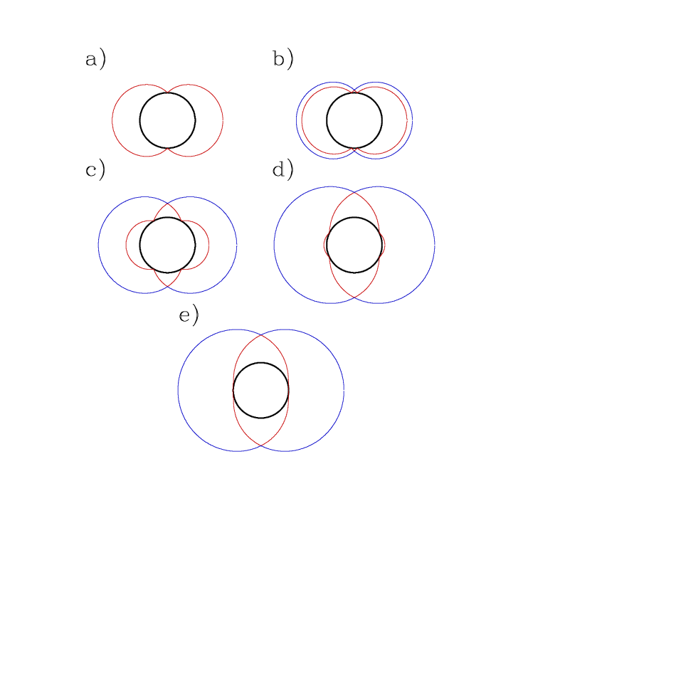

As discussed in the Introduction, the B-phase may evolve either from the A-phase, with , or directly from the normal phase, in which case . We now discuss these two scenarios in detail.
The order parameter of the AB transition is , which increases continuously from zero at the phase transition. The two degenerate cusp nodes in the directions in the A-phase (Fig. 1a) split into four non-degenerate cusp nodes in the B-phase at the phase transition (Fig. 1b).
The order parameter of the normalB transition is . In this case, the B-phase resembles the phase of octahedral systems corresponding to the three-dimensional representations with components . In the Landau potential, the difference between octahedral and tetrahedral appears only in sixth order and higher terms in the order parameter.Sergienko2004 Near the normal-to-superconducting phase transition, when all components of the order parameter are small, the growth of the order parameter is governed by fourth order terms in the Landau potential, which are identical for octahedral and tetrahedral systems, so at the phase transition in both cases. The difference between the gap functions of octahedral and tetrahedral systems with 3D order parameter components is due to a difference in the basis functions (7): in octahedral systems. Thus the octahedral phase has two non-degenerate smooth nodes in the directions shown in Fig. 1e), while the tetrahedral system has four cusp nodes (Figs. 1b-1d).
Thus the main difference between the two possible scenarios is the positioning of the nodes at the onset of the B-phase. In the normalAB scenario, the nodes will always be found in pairs near the directions (Fig. 1b), while in the normalB scenario, the positions of the four nodes are arbitrary (Fig. 1b-1d) and depend on the parameters and .
III Density of states
The low temperature form of the density of states (DOS) in superconductors is governed by the presence of nodes.Sigrist1991; Barash1996; Joynt2002 In general, cusp-like point nodes give rise to a quadratic dependence on energy.
III.1 A-phase
The gap function of the A-phase (8) is unitary and non-degenerate (Fig. 1a). Since the main contributions to the integral come from the vicinity of the nodes, the integral over can be split into two separate regions centred over each node, which are cut off such that the total integrated region in -space equals the Brillouin zone.Durst The nodes are degenerate and the contributions from each node are equal,
| (11) | |||||
where and are the momenta parallel and perpendicular to the Fermi surface at the node, , and . Changing variables again and using , , we find
| (12) | |||||
| (13) |
where the cutoff is finally introduced in the last equation. This result is equivalent to the usual result for a degenerate cusp node, ,Joynt2002 apart from a factor of two because there are two degenerate nodes in our calculation. In our case, the gap velocity, defined by is not the same in all directions since the node is not rotationally symmetric, and so the geometric average appears.
Eq. 13 is the density of states of the phase () at low temperatures. However, according to the considerations outlined in Section I, this phase is identified as the A-phase, which is only found in a narrow region of phase space just below . Therefore, Eq. 13 is not expected to be observed in PrOs4Sb12.
III.2 B-Phase
In triplet, non-unitary phases, in general, the gap function is non-degenerate, except along some lines on the Fermi surface. All nodes are found in the lower energy branch of the gap function , and the higher energy branch is usually neglected. However, if the nodes are found near the line where the gaps are degenerate then both gaps should be taken into account.
To find the density of states in the B-phase, we should consider the two different scenarios, normalA-phaseB-phase or normalB-phase, separately. In the former scenario, , and pairs of nodes are found on opposite sides of the Fermi surface. The partners in each pair are very close to each other and close to the gap degeneracy line, as shown in Fig. 1b). In this case, the higher energy gap should not be neglected. In the normalB-phase scenario, the positions of the nodes depend on the parameters and which are arbitrary.
III.2.1 normalA-phaseB-phase
At the onset of the B-phase , and we will assume that . Then the pairs of nodes are found in the vicinity of in the plane , as shown in Fig. 1b). The integration over -space is divided into four regions, which overlap for nodes within a pair.
The gap function in the vicinity of the nodes for the case when can be approximated by
| (14) |
where and
| (15) |
With this approximation, the ‘’ branch of the gap function continues smoothly to the ‘’ branch of the gap function at the line where the gap function is degenerate. Then two difficulties are overcome at once: both branches of the gap function are taken into account, and the contributions from each integration region are distinct, even though the regions overlap. Each region yields the same contribution to the density of states,
| (16) |
where , and as before. Then performing the same change of variables as in the A-phase calculation, we find
| (17) |
Note that in the limit we recover the A-phase result, as expected.
III.2.2 normal B-phase
In this situation, near the phase transition we have , however the positions of the nodes depend on the parameters and , which are completely undetermined. Then there are three possibilities to consider. The first is shown in Fig. 1b), where the nodes appear in pairs such that the pairs are close to the gap degeneracy line (if or ); in this case the above calculation is valid and the result (17) is obtained for ,
| (18) |
Second, when all four nodes are spaced far apart as shown in Fig. 1c), then the above calculations are again valid and the result (18) is obtained.
Finally, the nodes may appear in pairs which are far away from the gap degeneracy line, as shown in Fig. 1d). In this case the above treatment is invalid. Here we have a crossover between and , which is the behaviour of the limiting case shown in Fig. 1e), i.e., the octahedral phase , with smooth (quadratic) nodes. Such behaviour is not observed in experiments, which could mean that either the components of the order parameter are unequal (normalA-phaseB-phase scenario) or .
IV Specific heat and nuclear spin relaxation rate
The specific heat at low temperatures is given bySigrist1991
| (19) |
| (20) |
for the A-phase, and
| (21) |
for the B-phase.
The longitudinal nuclear spin-lattice relaxation rate is given bySigrist1991
| (22) |
In the limit of small nuclear resonance frequency , one finds
| (23) |
in the A-phase, while in the B-phase it is
| (24) |
These expressions give the low temperature behaviour of the specific heat and nuclear relaxation rate in terms of the tetrahedral parameters and and the order parameter components and .
V Domains
Directional dependent measurements are the ideal way to observe the anisotropy of the gap function. However, such measurements may be confounded by the presence of domains, different regions in space where the components of the order parameter are interchanged. In this section we offer a brief discussion of domains for the A-phase and the B-phase.
The A-phase has three different domains , and , which, in the absence of unusual crystal shape or external fields, are all expected to be present, and will lead to the observation of the full tetrahedral symmetry. Six (degenerate) nodes will be observed in the directions . Now let us suppose that there is some kind of external effect along the -axis which effectively lowers the symmetry from to . In an octahedral system, either the single domain , with nodes in the directions will be favoured, or the other two domains, and will be favoured. In the latter case, four nodes would be observed in the directions and . However, because the crystal symmetry of PrOs4Sb12 is tetrahedral to begin with, any axial perturbation will lift the degeneracy of all three domains, any of which could be favoured. Therefore, in the A-phase, if all domains are present then tetrahedral symmetry with six nodes will be observed. Otherwise, only one domain is present, the symmetry will be , with two nodes. It is not likely that two out of three domains would be present in the A-phase, but could be possible if they were very close in energy.
The same arguments also hold for the more complicated B-phase. Six domains are possible, with twenty-four non-degenerate nodes. If there is a single domain, then the symmetry is , and four nodes will be present.
VI Conclusions
In this article, we have attempted to give a physical description and comparison of the sequences of phase transitions normal and normal, which we identify with the phase transitions seen in experiments, normalAB or normalB, respectively. Although this description is derived entirely from basic considerations of symmetry, a complicated gap structure emerges with several unusual features. First, the positions of the nodes in the B-phase are not located on any symmetry axes. Although this is allowed by symmetry to occur in crystals with other point groups, such a feature has never before been considered. Second, because the B-phase is triplet and non-unitary, there are two non-degenerate gaps. The only known example of this is Sr2RuO4, but in that case the two gaps remain close in energy.Mackenzie2003 In PrOs4Sb12, for a direct normalB transition, the energy difference is expected to be large. Finally, the proposed AB transition, which is characterised by the splitting into two of the degenerate nodes of the the A-phase, is highly unusual.
In summary, we have proposed phase transition sequences in accordance with experimental evidence available to date and studied its basic properties. Superconductivity is best-described by a three component order parameter in the triplet channel. The superconducting phase has symmetry, is non-unitary, and has four cusp nodes at unusual points on the Fermi surface. The presence of nodes leads to a quadratic dependence on energy in the density of states, and power law behaviour in the specific heat and nuclear spin relaxation rate. There is also a second, higher energy, nodeless gap which may be experimentally accessible.
Acknowledgements.
We thank Ivan Sergienko for assistance with the proof in the Appendix and Ilya Vekhter for helpful discussions. This work was supported by NSERC of Canada.Appendix A Proof of the existence of nodes in the phase in the triplet channel
In Section II, we found the gap function using basis functions given by (7), and order parameter components . The gap function takes the form (9), which vanishes either in the plane at the points defined by when , or in the plane at the points when . In Section II, only p-wave pairing (basis functions linear in ) was considered. In order to rigorously demonstrate the existence of nodes all possible higher order pairings must be included in the basis functions. We now consider this most general case.
The most general form for the basis functions of the representation in is
| (25) | |||||
| (26) | |||||
| (27) | |||||
where is odd in , is odd in and even in and , and is odd in and even in and . Eventually, we will find solutions to where one of the ’s is zero (in agreement with the particular case of lowest order in basis functions (7)), so we set now.
Using (4), (6) and (25-27) one finds
| (28) | |||||
Case 1: : vanishes and
| (29) |
Nodes are found where , or where the function
| (30) |
vanishes.
Case 2: : vanishes and
| (31) |
Nodes are found where , or where the function
| (32) |
vanishes.
We have
If , then changes sign, i.e., there is a node of in the plane somewhere between the positions and . Symmetry requires that there be (at least) four nodes on the Fermi surface. If , then changes sign, i.e., there are four nodes in the plane.
Thus we have proved that, in general, the triplet phase with order parameter components has four nodes in either the plane or at the positions or , where and depend on the particular form of the basis functions. These nodes are “approximate”, in the sense that they are a consequence of symmetry and follow from the most general basis functions for the representation. These nodes are also “rigorous”, since the state couples to no secondary superconducting order parameters.Sergienko2004
References
- (1) M. B. Maple, E. D. Bauer, V. S. Zapf, E. J. Freeman, N. A. Frederick and R. P. Dickey, Acta. Phys. Pol. 32, 3291 (2001).
- (2) E. D. Bauer, N. A. Frederick, P.-C. Ho, V. S. Zapf, and M. B. Maple, Phys. Rev. B 65, 100506(R) (2002).
- (3) K. Izawa, Y. Nakajima, J. Goryo, Y. Matsuda, S. Osaki, H. Sugawara, H. Sato, P. Thalmeier, and K. Maki, Phys. Rev. Lett. 90, 117001 (2003).
- (4) Y. Aoki, A. Tsuchiya, T. Kanayama, S. R. Saha, H. Sugawara, H. Sato, W. Higemoto, A. Koda, K. Ohishi, K. Nishiyama, and R. Kadono, Phys. Rev. Lett. 91, 067003 (2003).
- (5) E. E. M. Chia, M. B. Salamon, H. Sugawara, and H. Sato, Phys. Rev. Lett. 91, 247003 (2003).
- (6) A. D. Huxley, M.-A. Measson, K. Izawa, C. D. Dewhurst, R. Cubitt, B. Grenier, H. Sugawara, J. Flouquet, Y. Matsuda and H. Sato, Phys. Rev. Lett. 93, 187005 (2004).
- (7) M. Nishiyama, T. Kato, H. Sugawara, D. Kikuchi, H. Sato, H. Harima, and G.-q. Zheng, J. Phys. Soc. Jpn. 74, 1938 (2005).
- (8) N. A. Frederick, T. A. Sayles and M. B. Maple, Phys. Rev. B 71, 064508 (2005).
- (9) W. Higemoto, S. R. Saha, A. Koda, K. Ohishi, R. Kadono, Y. Aoki, H. Sugawara and H. Sato, Phys. Rev. B 75, 020510(R) (2007).
- (10) K. Katayama, S. Kawasaki, M. Nishiyama, H. Sugawara, D. Kikuchi, H. Sato, and G.-q. Zheng, J. Phys. Soc. Jpn. 76, 023701 (2007).
- (11) D. E. MacLaughlin, J. E. Sonier, R. H. Heffner, O. O. Bernal, B.-L. Young, M. S. Rose, G. D. Morris, E. D. Bauer, T. D. Do and M. B. Maple, Phys. Rev. Lett. 89, 157001 (2002).
- (12) H. Suderow, S. Viera, J. D. Strand, S. Bud’ko and P. C. Canfield, Phys. Rev. B 69, 060504 (2004).
- (13) H. Kotegawa, M. Yogi, Y. Imamura, Y. Kawasaki, G.-q. Zheng, Y. Kitaoka, S. Ohsaki, H. Sugawara, Y. Aoki, and H. Sato, Phys. Rev. Lett. 90, 027001 (2003).
- (14) Y. Aoki, T. Namiki, S. Ohsaki, S. R. Saha, H. Sugawara and H. Sato, J. Phys. Soc. Jpn. 71, 2098 (2002).
- (15) R. Vollmer, A. Fait, C. Pfleiderer, H. v. Löhneysen, E. D. Bauer, P.-C. Ho, V. Zapf, and M. B. Maple, Phys. Rev. Lett. 90, 057001 (2003).
- (16) T. Tayama, T. Sakakibara, H. Sugawara, Y. Aoki and H. Sato, J. Phys. Soc. Jpn. 72, 1516 (2003).
- (17) P.-C. Ho, N. A. Frederick, V. S. Zapf, E. D. Bauer, T. D. Do, M. B. Maple, A. D. Christianson, and A. H. Lacerda, Phys. Rev. B 67, 180508(R) (2003).
- (18) N. Oeschler, P. Gegenwart, F. Weickert, I. Zerec, P. Thalmeier, F. Steglich, E. D. Bauer, N. A. Frederick and M. B. Maple, Phys. Rev. B 69, 235108 (2004).
- (19) K. Grube, S. Drobnik, C. Pfleiderer, H. v. Löhneysen, E. D. Bauer and M. B. Maple, Phys. Rev. B 73, 104503 (2006).
- (20) M.-A. Measson, D. Braithewaite, J. Flouquet, G. Seyfarth, J. P. Brison, E. Lhotel, C. Paulsen, H. Sugawara and H. Sato, Phys. Rev. B 70, 064516 (2004).
- (21) G. Seyfarth, J. P. Brison, M.-A. Measson, J. Flouquet, K. Izawa, Y. Matsuda, H. Sugawara, and H. Sato, Phys. Rev. Lett. 95, 107004 (2005).
- (22) G. Seyfarth, J. P. Brison, M.-A. Méasson, D. Braithewaite, G. Lapertot and J. Flouquet, Phys. Rev. Lett. 97, 236403 (2006).
- (23) M. Yogi, T. Nagai, Y. Imamura, H. Mukuda, Y. Kitaoka, D. Kikuchi, H. Sugawara, Y. Aoki, H. Sato and H. Harima, J. Phys. Soc. Jpn. 75, 124702 (2006).
- (24) J. Goryo, Phys. Rev. B 67, 184511 (2003).
- (25) M. Ichioka, N. Nakai and K. Machida, J. Phys. Soc. Jpn. 72, 1322 (2003).
- (26) K. Miyake, H. Kohno and H. Harima, J. Phys.: Condens. Matter 15, L275 (2003).
- (27) K. Maki, S. Haas, D. Parker, H. Won, K. Izawa and Y. Matsuda, Europhys. Lett. 68, 720 (2004).
- (28) M. Matsumoto and M. Koga, J. Phys. Jpn. 73, 1135 (2004); M. Matsumoto and M. Koga, J. Phys. Jpn. 74, 1686 (2005); M. Koga, M. Matsumoto and H. Shiba, J. Phys. Soc. Jpn. 75, 014709 (2006).
- (29) P. Thalmeier, Physica B 378-380, 261 (2006).
- (30) G. E. Volovik and L. P. Gor’kov, Sov. Phys. JETP 61, 843 (1985); Yu. M. Gufan, JETP 80, 485 (1995).
- (31) M. Sigrist, and K. Ueda, Rev. Mod. Phys., 63, 239 (1991)
- (32) I. A. Sergienko and S. H. Curnoe, Phys. Rev. B, 70, 144522 (2004); see Ref. error.
- (33) S. H. Curnoe, T. R. Abu Alrub, I. A. Sergienko and I. Vekhter, J. Magn. Magn. Mater. 310, 605 (2007).
- (34) There is an error in Table I of Ref. [Sergienko2004]. The triplet-paired phase with symmetry was reported to be nodeless. However, it does in fact have four point nodes (approximate and rigorous) at the positions . This result can be proved rigorously as a strict consequence of symmetry (see Appendix A). This error lead to our claim [curnoe2006] that the nodes lift away from the Fermi surface to form deep dips in the gap function at the A-B transition.
- (35) V. Kuznetsova and V. Barzykin, Europhys. Lett. 72 (3), 437 (2005).
- (36) S. Mukherjee and D. F. Agterberg, Phys. Rev. B 74, 174505 (2006).
- (37) Yu. S. Barash, and A. A. Svidzinsky, Phys. Rev. B, 53, 15254 (1996).
- (38) R. Joynt, and L. Taillefer, Rev. Mod. Phys. 74, 235 (2002).
- (39) A. C. Durst and P. A. Lee, Phys. Rev. B 62 1270 (2000).
- (40) A. P. Mackenzie and Y. Maeno, Rev. Mod. Phys. 75, 657 (2003).